TECHNISCHE UNIVERSIT ¨AT ILMENAU Institut f¨ur Praktische Informatik und Medieninformatik
Fakult¨at f¨ur Informatik und Automatisierung Fachgebiet Datenbanken und Informationssysteme
Dissertation
Finding the Right Processor for the Job —
Co-Processors in a DBMS
vorgelegt von Dipl.-Inf. Hannes Rauhe geboren am 5.9.1985 in Meiningen zur Erlangung des akademischen Grades
Dr.-Ing.
1. Gutachter: Prof. Dr.-Ing. habil. Kai-Uwe Sattler 2. Gutachter: Prof. Dr.-Ing. Wolfgang Lehner 3. Gutachter: Prof. Dr. Guido Moerkotte
Abstract
Today, more and more Database Management Systems (DBMSs) keep the data com-pletely in memory during processing or even store the entire database there for fast access. In such system more algorithms are limited by the capacity of the processor, be-cause the bottleneck of Input/Output (I/O) to disk vanished. At the same time Graphics Processing Units (GPUs) have exceeded the Central Processing Unit (CPU) in terms of processing power. Research has shown that they can be used not only for graphic pro-cessing but also to solve problems of other domains. However, not every algorithm can be ported to the GPU’s architecture with benefit. First, algorithms have to be adapted to allow for parallel processing in a Single Instruction Multiple Data (SIMD) style. Sec-ond, there is a transfer bottleneck because high performance GPUs are connected via PCI-Express (PCIe) bus.
In this work we explore which tasks can be offloaded to the GPU with benefit. We show, that query optimization, query execution and application logic can be sped up under certain circumstances, but also that not every task is suitable for offloading. By giving a detailed description, implementation, and evaluation of four different examples, we explain how suitable tasks can be identified and ported.
Nevertheless, if there is not enough data to distribute a task over all available cores on the GPU it makes no sense to use it. Also, if the input data or the data generate during processing does not fit into the GPU’s memory, it is likely that the CPU produces a result faster. Hence, the decision which processing unit to use has to be made at run-time. It is depending on the available implementations, the hardware, the input parameters and the input data. We present a self-tuning approach that continually learns which device to use and automatically chooses the right one for every execution.
Abbreviations
AES Advanced Encryption Standard AVX Advanced Vector Extensions BAT Binary Association Table
BLAS Basic Linear Algebra Subprograms CPU Central Processing Unit
CSV Comma Separated Values
DBMS Database Management System DCM Decomposed Storage Model ETL Extract, Transform, Load
FLOPS Floating Point Operations per Second FPGA Field-Programmable Gate Array FPU Floating Processing Unit
GPU Graphics Processing Unit
GPGPU General Purpose Graphics Processing Unit HDD Hard Disk Drive
I/O Input/Output JIT Just-In-Time
LWC Light-Weight Compression
MMDBMS Main Memory Database System ME Maximum Entropy
MIC Many Integrated Core MVS Multivariant Statistics NOP No Operation
OLTP Online Transactional Processing OLAP Online Analytical Processing ONC Open-Next-Close
OS Operating System PCIe PCI-Express
PPE PowerPC Processing Element QEP Query Execution Plan
QPI Intel QuickPath Interconnect RAM Random Access Memory
RDBMS Relational Database Management System RDMA Remote Direct Memory Access
SIMD Single Instruction Multiple Data SMX Streaming Multi Processor SPE Synergistic Processing Element SQL Structured Query Language SSD Solid State Drive
SSE Streaming SIMD Extensions STL Standard Template Library TBB Intel’s Thread Building Blocks UDF User-Defined Function
Contents
1. Introduction 1
1.1. Motivation . . . 1
1.2. Contributions . . . 2
1.3. Outline . . . 4
2. Main Memory Database Management Systems 5 2.1. OLTP and OLAP . . . 5
2.2. Main Memory DBMS for a Mixed Workload . . . 7
2.2.1. SAP HANA Architecture . . . 8
2.2.2. Columnar Storage . . . 10
2.2.3. Compression . . . 11
2.2.4. Main and Delta Storage . . . 16
2.3. Related Work: Using Co-processors in a DBMS . . . 17
3. GPUs as Co-Processors 19 3.1. SIMD Processing and Beyond . . . 19
3.1.1. Flynn’s Taxonomy . . . 20
3.1.2. Hierarchy of Parallelism—the GPU Architecture . . . 21
3.1.3. Programming Model for GPU Parallelsim . . . 22
3.2. Communication between CPU and GPU . . . 23
3.3. Software Frameworks and Libraries . . . 24
3.4. Micro-Benchmarks . . . 26
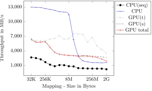
3.4.1. Memory Bandwidth and Kernel Overhead . . . 26
3.4.2. Single Core Performance . . . 28
3.4.3. Streaming . . . 29
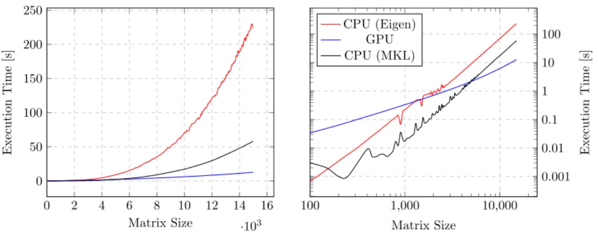
3.4.4. Matrix Multiplication . . . 32
3.4.5. String Processing . . . 33
3.5. DBMS Functionality on GPUs . . . 37
3.5.1. Integrating the GPU for Static Tasks into the DBMS . . . 39
3.5.2. Re-Designing Dynamic Tasks for Co-Processors . . . 41
3.5.3. Scheduling . . . 42
4. Integrating Static GPU Tasks Into a DBMS 43 4.1. GPU Utilization with Application Logic . . . 44
4.1.1. External Functions in IBM DB2 . . . 44
4.1.2. K-Means as UDF on the GPU . . . 45
4.1.4. Evaluation . . . 49
4.1.5. Conclusion . . . 50
4.2. GPU-assisted Query Optimization . . . 52
4.2.1. Selectivity Estimations and Join Paths . . . 52
4.2.2. Maximum Entropy for Selectivity Estimations . . . 53
4.2.3. Implementation of the the Newton Method . . . 54
4.2.4. Evaluation . . . 55
4.2.5. Conclusion . . . 56
4.3. The Dictionary Merge on the GPU: Merging Two Sorted Lists . . . 57
4.3.1. Implementation . . . 57
4.3.2. Evaluation . . . 61
4.3.3. Conclusion . . . 62
4.4. Related Work . . . 62
5. Query Execution on GPUs—A Dynamic Task 65 5.1. In General: Using GPUs for data-intensive problems . . . 66
5.2. JIT Compilation—a New Approach suited for the GPU . . . 67
5.3. A Model for Parallel Query Execution . . . 69
5.4. Extending the Model for GPU Execution . . . 71
5.4.1. Concrete Example . . . 73
5.4.2. Limitations of the GPU Execution . . . 75
5.5. Evaluation . . . 76
5.5.1. Details on Data Structures . . . 76
5.5.2. Test System and Test Data . . . 76
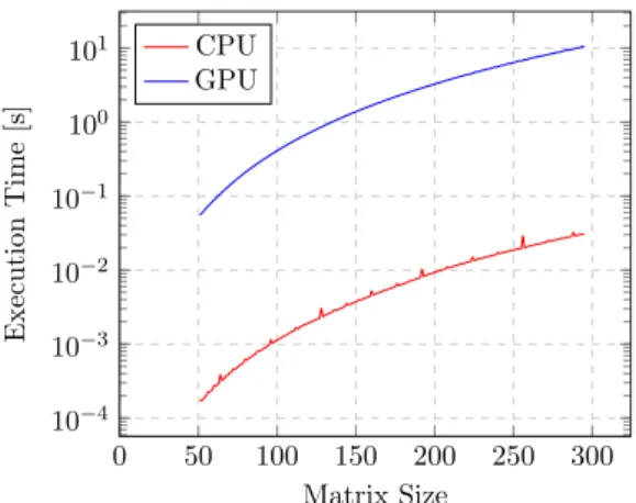
5.5.3. GPU and CPU Performance . . . 77
5.5.4. Number of Workgroups and Threads . . . 78
5.5.5. The Overhead for Using the GPU . . . 79
5.6. Related Work . . . 79
5.7. Conclusion . . . 81
6. Automatically Choosing the Processing Unit 83 6.1. Motivation . . . 83 6.2. Operator Model . . . 85 6.2.1. Base Model . . . 85 6.2.2. Restrictions . . . 87 6.3. Decision Model . . . 88 6.3.1. Problem Definition . . . 88
6.3.2. Training and Execution Phase . . . 89
6.3.3. Model Deployment . . . 91
6.4. Evaluation . . . 92
6.4.1. Use Cases for Co-Processing in DBMS . . . 92
6.4.2. Implementation and Test Setup . . . 95
6.4.3. Model Validation . . . 96
Contents 6.5. Related Work . . . 98 6.6. Conclusions . . . 99 7. Conclusion 101 Bibliography 103 A. Appendix 113
1. Introduction
In the 1970s the idea of a database machine was a trending topic in research. The hardware of these machines was supposed to be built from ground up to serve only one purpose: efficiently accessing and processing data stored in a Database Management System (DBMS). One of the common ideas of the different designs proposed was the usage of a high number of processing units in parallel. The evolution of the Central Processing Unit (CPU) and disks overtook the development of these database machines and in the 80s, the idea was declared a failure [11]. Thirty years later researchers again proposed to use a massively parallel architecture for data processing, but this time, it was already available: the Graphics Processing Unit (GPU). However, except for some research systems there is still no major DBMS that runs on GPUs.
We think that the reason for this is the versatility of modern DBMS. An architecture for DBMS must be able to do every task possible reasonably well, whether it is aggregat-ing data, simple filteraggregat-ing, processaggregat-ing transactions, complex mathematical operations, or the collection and evaluation of statistics on the data stored in the system. A specialized processor may be able to do a subset of these tasks very fast, but then it will fail to do the rest. The GPU is able to process a huge amount of data in parallel, but it has problems with short transactions, which are not suitable for parallel processing, because they require a consistent view on the data.
However, nowadays different processing units are available in one system. In recent research therefore the focus switched to the usage of heterogeneous hardware and the concept of co-processing. Instead of calculating all by itself, the CPU orchestrates a number of different processing units within the system and decides for each task, where to execute it. The question therefore not longer is: “How does the perfect processor for a DBMS look?”, but
“Which of the available processor is the right one to use for a certain task?”.
1.1. Motivation
On the one hand there are many different tasks a DBMS has to process to store data and keep it accessible. There are the operators used for query execution, such as selection, join, and aggregation with simple or complex predicates. Under the hood the systems executes much more logic to maintain stored data and collect meta data on how users access the content. These statistics are used to optimize the query execution; partly with complex mathematical methods. Additionally, most vendors position their DBMS more and more as a data management platform that is not only able to execute queries but any application logic defined by the user as well.
On the other hand every standard PC can be equipped with powerful co-processors, specialized on a certain domain of algorithms. Almost any modern PC already has a GPU which is able to solve general purpose algorithms with the help of its massively par-allel architecture. Additionally, there are Field-Programmable Gate Arrays (FPGAs), Intel’s Xeon Phi, or IBM’s Cell processor. Of course, any task can be solved by the CPU, but since its purpose is so generic, other hardware may be
• cheaper,
• more efficient in terms of memory consumption,
• or simply faster
at executing the task. Even if the co-processor is just as good as the CPU for a certain problem; if it is available in the system anyhow it can be used to free resources on the CPU for other jobs.
However, in contrast to co-processors that are integrated into the CPU—such as the Floating Processing Unit (FPU) or cryptography processors, e.g., for accelerating Ad-vanced Encryption Standard (AES)–the co-processors mentioned in the last paragraph cannot be used by just re-compiling the code with special instructions. Instead, they require their own programming model and special compilers. That means that most algorithms have to be re-written to run on co-processors. This re-write is not trivial, because especially GPU algorithms require a completely different approach. Since the prediction of the performance of those new algorithm is impossible due to the complexity of the hardware, there are three questions to answer:
• Which tasks can be ported to a co-processor and how is this done?
• Which tasks are likely and which are unlikely to benefit from another architecture?
• How can the system automatically decide on the best processing unit to use for a specific task?
At the moment, the data to be processed by a task usually has to be copied to the co-processor, so data-intensive tasks are usually unlikely to benefit from the GPU.
However, since we reached a peak of single-thread CPU performance because of physics [57], CPU vendors are changing their architectures to support for instance vec-torized and multi-threaded execution. These concepts are already built to an extreme in GPUs and FPGAs. In heterogeneous architectures, GPUs are integrated into the CPU, e.g., AMD’s Fusion architecture [14]. Hence, modifications to simple algorithms or completely new algorithms for co-processor architectures will play a key role in the future for CPU development as well.
1.2. Contributions
In this thesis we take a deep look into using the GPU as co-processor for DBMS oper-ations. We compare the architecture and explain, where the GPU is good at and when
1.2. Contributions
it is better to use the CPU. By doing a series of micro benchmarks we compare the performance of a GPU to typical server CPUs. Against popular opinion the GPU is not necessarily always better for parallel compute-intensive algorithms. Modern server CPUs provide a parallel architecture with up to 8 powerful cores themselves. With the help of the benchmarks we point out a few rules of thumb to identify good candidates for GPU execution.
The reason that the GPU provides so much raw power is that hundreds of cores are fitted onto one board. These cores are simple and orders of magnitude slower than a typical CPU core and because of their simplicity they do not optimize the execution of instructions. Where the CPU uses branch-prediction and out-of-order-execution, on the GPU each instruction specifies what one core does and when. Additionally porting an algorithm to the Single Instruction Multiple Data (SIMD) execution model often involves overhead. Missing optimization and the necessary overhead usually mean that only a fraction of the theoretical power can actually be used. Hence the code itself has to be highly optimized for the task. Because of this we have to differentiate between static tasks that always execute the same code branches in the same order, and dynamic tasks such as query execution, where modular code blocks are chained and executed depending on the query.
For static tasks we show candidates from three different classes: application logic, query optimization, and a maintenance task. While the first two can benefit from the GPU for certain input parameters, the maintenance task is not only data-intensive but also not “compatible” to the GPU’s architecture. For dynamic tasks we propose code generation and Just-In-Time (JIT)-compilation to let the compiler optimize the code for the specific use case at run-time. In any case: if the input for a task is too small, not all cores on the GPU can be used and performance is lost. Hence, we have to decide each time depending on the input whether it is worth using the GPU for the job. In the last part of this thesis we present a framework which automatically makes a decision based on predicted run-times for the execution.
We show that
• there is a huge difference between parallel algorithms for the CPU and the GPU.
• application logic can be executed by the DBMS and on the GPU with advantages from both concepts.
• query optimization can benefit from the performance the GPU provides in combi-nation with a library for linear algebra.
• there are tasks that simply cannot benefit from the GPU; either because they are data intensive or because they are just not compatible to the architecture.
• we can execute queries completely on the GPU, but there are limits for what can be done with our approach.
• the system can learn, when using the co-processor for a certain task is beneficial and automatically decide, where to execute a task.
In every evaluation we aim for a fair comparison between algorithms optimized for and running on a modern multi-core CPU against GPU-optimized algorithms. Because DBMS usually run on server hardware, we use server CPUs and GPUs; details are explained in Section 6.1 and in the Appendix.
1.3. Outline
In Chapter 2 we start off with explaining the environment for our research: while in disk-based DBMS most tasks were Input/Output (I/O) bound, Main Memory Database System (MMDBMS) make stored data available for the CPU with smaller latency and higher bandwidth. Hence, processing power has a higher impact in these systems and investigating other processing units makes more sense than before.
The most popular co-processor at the moment, the GPU, is explained in detail in Chapter 3. We start with the details about its architecture and the way it can be used by developers. With a series of benchmarks we give a first insight on how a GPU performs in certain categories compared to a CPU. Based on these findings we explain the further methodology of our work in Section 3.5. The termsstatic and dynamic task are explained there.
In Chapter 4 we take a deep look at candidates of three different classes of static tasks within a DBMS and explain how these algorithms work and perform on a GPU. While some application logic and query optimization can benefit from the GPU for certain input parameters, the maintenance task is not only data-intensive but also not “compatible” to the GPU’s architecture. Even without the transfer bottleneck, the CPU would be faster and more efficient in processing.
However, the most important task of any DBMS is query execution, which we consider to be a dynamic task. Because of the GPU’s characteristics we cannot use the approach of executing each database operator on its own as explained in Section 5.2. Instead we use the novel approach of generating code for each individual query and compile it at run-time. We present the approach, its advantages, especially for the GPU, as well as its limitations in Chapter 5.
Most tasks are not simply slower or faster on the GPU. Instead, it depends on the size of the input data and certain parameters that can only be determined at run-time. Because of the unlimited number of different situations and hardware-combinations we cannot decide at compile time, when to use which processing unit. The framework HyPE decides at run-time and is presented in Chapter 6.
2. Main Memory Database Management
Systems
Relational Database Management Systems (RDBMSs) today have to serve a rich variety of purposes. From simple user-administration and profile storage in a web community forum to complex statistical analysis on costumer and sales data in world-wide acting corporations anything can be found. For a rough orientation the research community categorizes scenarios under two different terms: Online Transactional Processing (OLTP) and Online Analytical Processing (OLAP). Until recently there was no system that could serve both workloads efficiently. If a user wanted to do both types of queries on the same data, replication from one system to another was needed. Nowadays, the target of the major DBMS vendors is to tackle both types efficiently in one system. The bottleneck of I/O operations in traditional disk-based DBMS makes it impossible to achieve this goal.
The concept of the MMDBMS eliminates this bottleneck and gives the computational power of the processor a new higher priority. Because I/O operations are cheaper on Random Access Memory (RAM), processes that were I/O-bound in disk-based system are often CPU-bound in MMDBMS. Co-processor provide immense processing speeds for problems of their domain. Their integration into a MMDBMS is a new chance to gain better performance for such CPU-bound tasks.
In this chapter, we explain how MMDBMSs work and what possibilities and chal-lenges arise because of their architecture. In the first section we explain the difference between OLTP and OLAP workloads, which is necessary for a basic understanding of the challenges DBMS researchers and vendors face. The following Section 2.2 explains the recent changes in hardware that explain the rising interest in MMDBMSs. We take a look at the architecture and techniques used in HANA to support both scenarios, so-called mixed workloads.
For this thesis we focus on the GPU as co-processor, but there are of course other candidates. Before we get to the details of GPUs in the next chapter, we take a look at noticeable attempts that were already made to integrate different types of co-processors into a DBMS in Section 2.3.
2.1. OLTP and OLAP
Based on characteristics and requirements for a DBMS there are two fundamentally different workloads: OLTP and OLAP.
A DBMS designed for OLTP must be able to achieve a high throughput of read and— at the same time—write transactions. It must be able to keep the data in a consistent
state at every time and make sure that no data is lost even in case of a power failure or any other interruption. Additionally, transactions do not interfere in each others processing and are only visible, when they are completed successfully. These characteristics are know under the acronym ACID: Atomicity, Consistency, Isolation and Durability [41]. Users and applications that used RDBMSs rely on the systen to act according to these rules. Typical Structured Query Language (SQL) statements of a OLTP workload are shown in Listing 2.1. They are a mixture of accessing data with simple filter criteria, updating existing tuples and the insertion of new records into the system.
Listing 2.1: Typical OLTP queries 1 S E L E C T * F R O M c u s t o m e r
2 W H E R E c u s t o m e r _ i d = 1 2 ; 3
4 I N S E R T I N T O c u s t o m e r ( name , address , city , zip )
5 V A L U E S ( " C u s t Inc " , " Pay R o a d 5 " , " B i l l t o w n " , 5 5 5 ) ; 6
7 U P D A T E c u s t o m e r SET c u s t o m e r _ s t a t u s = " g o l d " 8 W H E R E n a m e = " Max M u s t e r m a n n " ;
The requirements for a OLAP-optimized DBMS are different. Instead of simple and short transactions, they must support the fast execution of queries that analyze huge amounts of data. But in contrast to OLTP scenarios the stored data is not or only rarely changed. Therefore, the ACID rules do not play an important role in analytic scenarios. Compared to a OLTP scenario there are less queries, but every query accesses large amounts of data and usually involves much more calculations due to its complexity. A typical OLAP-query is shown in Listing 2.2.
Listing 2.2: Query 6 of the TPC-H benchmark [100] 1 S E L E C T sum ( l _ e x t e n d e d p r i c e * l _ d i s c o u n t ) as r e v e n u e 2 F R O M l i n e i t e m 3 W H E R E l _ s h i p d a t e >= d a t e ’ :1 ’ 4 AND l _ s h i p d a t e < d a t e ’ :1 ’ + i n t e r v a l ’ 1 ’ y e a r 5 AND l _ d i s c o u n t B E T W E E N :2 - 0 . 0 1 AND :2 + 0 . 0 1 6 AND l _ q u a n t i t y < :3;
Although classic RDBMSs support OLTP and OLAP workloads, they are often not capable of providing an acceptable performance for analytical queries. Especially in enterprise scenarios another system is used that is optimized solely for OLAP. These so-called data warehouses use read-optimized data structures to provide fast access to the stored records. Furthermore, they are optimized to do calculations on/with the data while scanning it. Because the data structures used do not support fast changes, OLAP systems perform poorly at update- or write-intensive workloads. Therefore, the data that was recorded by the OLTP system(s) must be transferred regularly. This happens in form of batch inserts into the data warehouse. Since this process also involves some form
2.2. Main Memory DBMS for a Mixed Workload
of transformation to read-optimized schemes and data structures, it is called Extract, Transform, Load (ETL) [102]. The batch insert can contain data from a high number of different system. Their exports are converted and may be pre-processed, e.g., sorted and aggregated, before they are actually imported into the OLAP system [58].
A typical business example that shows the organization of different DBMS, is a global supermarket chain. Every product that is sold has to be recorded. However, the trans-action is not completed when the product is registered by the scanner at checkout, but when the receipt is printed. Until then it must be possible to cancel the transaction with-out any change to the inventory or the revenue. Additionally, in every store hundreds or thousands transaction are made every day. This is a typical OLTP workload for a DBMS. Similar scenarios can be found at a warehouse, where the goods are distributed to the stores in the region. Here, every incoming and outgoing product is recorded just in time. In contrast to that a typical OLAP-query is to find the store with the lowest profit of a certain region, or the product that creates the highest revenue in a month. This OLAP workload is usually handled by the data warehouse, which holds the records of all stores and warehouses.
This solution has disadvantages: since at least two DBMS are involved, there is no guarantee that data is consistent between both. During the ETL process, it must be ensured that no records are lost or duplicated. Additionally, because there is not one single source of truth, every query has to be executed in the right system. But the most significant disadvantage is that the more sources there are, the longer the ETL process takes. Hence, the time until the data is available for analysis gets longer, when more data is recorded. Especially in global companies real-time analytics1 are not available with this approach [83].
2.2. Main Memory DBMS for a Mixed Workload
Most systems today use Hard Disk Drives (HDDs) as primary storage, because they pro-vide huge amounts of memory at an affordable price. However, while CPU performance increased exponentially over the last years, HDD latency decreased and bandwidth in-creased only slowly. Table 2.1 lists the access latency of every memory type available in modern server hardware. There is a huge difference between HDD and RAM la-tency (and bandwidth as well), which is known as the memory gap. Therefore, the main performance bottleneck for DBMS nowadays (and at least in the last 20 years) is I/O. The first DBMSs that addressed this problem by holding all data in main mem-ory while processing queries were available in the 1980s [26]. These MMDBMSs do not write intermediate results, e.g., joined tables, to disk like traditional disk-based system and therefore reduce I/O, especially for analytic queries, where intermediate results can become very large.
In recent years the amount of RAM fitting into a single machine passed the 1 TB mark and became cheap enough to replace the HDD in most business scenarios. Hence, the
1
L1 Cache ≈4 cycles
L2 Cache ≈10 cycles
L3 Cache ≈40–75 cycles
L3 Cache via Intel QuickPath Interconnect (QPI) ≈100–300 cycles
RAM ≈60 ns
RAM via QPI ≈100 ns
Solid State Drive (SSD) ≈80 000 ns
HDD ≈5 000 000 ns
Table 2.1.: Approximation of latency for memory access (reads) [64, 30, 105] concept of MMDBMS was extended to not only keep active data in main memory, but use RAM as primary storage for all data in the system2.
For DBMS vendors this poses a new challenge, because moving the primary storage to RAM means tuning data structures and algorithms for main memory characteristics and the second memory gap between CPU-caches and RAM. MMDBMS still need a persistent storage to prevent data loss in case of a power failure, therefore every transaction still triggers a write-to-disk operation. Hence, OLTP workloads can by principle not benefit as much as OLAP, but modern hardware enables these systems to provide acceptable performance for OLTP as well.
In the next sections we show some of the principle design decisions of relational MMDBMS on the example of SAP HANA. While other commercial RDBMS started of as disc-oriented systems and added main memory as primary storage in their products— e.g., SQLServer with Hekaton [20], DB2 with BLU [86], and Oracle with Times Ten [80]— HANA is built from the ground up to use main memory as the only primary storage.
2.2.1. SAP HANA Architecture
On the one hand SAP HANA is a standard RDBMS that supports pure SQL and, for better performance, keeps all data—intermediate results as well as stored data—in main memory. Hence, the system provides full transactional behavior while being optimized for analytical workloads. The design supports parallelization ranging from thread and core level up to distributed setups over multiple machines. On the other hand HANA is a platform for data processing specialized to the needs of SAP applications [21, 92, 22]. Figure 2.1 shows the general SAP HANA architecture. The core of the DBMS are the In-Memory Processing engines, where relational data can either be stored row-wise or column-wise. Data is usually stored in the column store, which is faster for OLAP scenarios as we will explain in Section 2.2.2. However, in case of clear OLTP workloads, HANA also provides a row store. The user of the system has to decide, where a table is stored at creation time, while the system handles the transfer between the storage engines when a query needs data from both. Hence, the ETL-process is not necessary,
2
2.2. Main Memory DBMS for a Mixed Workload Metadata Manager MDX SQLScript ... Execution Engine Calculation Engine Optimizer and Plan Generator Connection and Session Management SQL Transaction Manager Persistence Authorization Manager
In-Memory Processing Engines
Column/Row Engine Graph Engine Text Engine
Business Applications
Logging and Recovery Data Storage
Figure 2.1.: Overview of the SAP HANA DB architecture [22]
resp. transparent to the users of the DBMS. Psaroudakis et al. showed how HANA handles both types of workloads at the same time [85].
As a data management platform, HANA allows graph data and text data to be stored in two specialized engines next to relational data. In every case, processing and storage are focused on main memory. If necessary tables can be unloaded to disk, but have to be copied to main memory again for processing. Because of this there is no need to optimized data structures in any way for fast disk access. Instead data structures as well as algorithms are built to be cache-aware to cope with the second memory gap. Furthermore, the engines compress the data using a variety of compression schemes. As we discuss in Section 2.2.3 this not only allows more data to be kept in main memory but speeds up query execution as well.
Applications communicate with the DBMS with the help of various interfaces. Stan-dard applications can use the SQL interface for generic data management functionality. Additionally, SQLScript [9] enables procedural aspects for data processing within the DBMS. More specialized languages for problems of a certain domain are MDX for pro-cessing data in OLAP cubes, WIPE to query graphs [90, 89], and even an R integration for statistics is available [39]. SQL queries are translated into an execution plan by the plan generator, which is then optimized and executed. Queries from other interfaces are eventually transformed into the same type of execution plan and executed in the same engine, but are first described by a more expressive abstract data flow model in the calculation engine. Independent of the interface, the execution engine handles the parallel execution and the distribution over several nodes.
On top of the interfaces there is the Component for Connection and Session Manage-ment, which is responsible for controlling individual connections between the database layer and the application layer. The authorization manager governs the user’s permis-sions and the transaction manager implements snapshot isolation or weaker isolation levels. The metadata manager holds the information about where tables are stored in which form and on which machine if the system was set up in a distributed landscape. All data is kept in main memory, but to guarantee durability in case of an (unexpected)
Col1 Col2 Col3 Row 1 A1 A2 A3 Row2 B1 B2 B3 Row3 C1 C2 C3 A1 A2 A3 B1 B2 B3 C1 C2 C3 A1 B1 C1 A2 B2 C2 A3 B3 C3 row-wise column-wise
Figure 2.2.: Row- vs. column-oriented storage
shutdown data needs to be stored on disk (HDD or SSD) as well. During savepoints and merge operations (see Section 2.2.4) tables are completely written to disk; in between updates are logged. In case of a system failure, these logs are replayed to recover the last committed state [22].
2.2.2. Columnar Storage
Since relations are two-dimensional structures there has to be a form of mapping to store them in the one-dimensional address space of memory. In general there are two different forms: either relations are stored row-wise or column-wise.
As shown in Figure 2.2 in row-wise storage all values of a tuple are stored contiguously in memory. The most significant advantage is that the read access to a complete row as well the insertion of a new row, which often happens in OLTP scenarios, can be processed efficiently. In contrast column stores store all values of a column contiguously in mem-ory. Therefore, access to a single row means collecting data from different positions in memory. In OLAP scenarios values of single attributes are regularly aggregated, which means that fast access to the whole column at once is beneficial. When queries access only a small number of columns in the table columnar storage allows to just ignore the other columns. Naturally, column stores have the advantage in these situations.
Main memory is still an order of magnitude more expensive than disk. Therefore, MMDBMSs use compression whenever possible before storing the data. In terms of compression, the columnar storage has an advantage: the information entropy of data stored within one column is lower than within one row. Every value is by definition of the same data type and similar to other values. Lower information entropy directly leads to better compression ratios [2]. It is easier, for instance, to compress a set of phone numbers than a set with a phone number, a name and an e-mail address. Additionally, often there is a default value that occurs in columns at a high frequency.
There are two different data layouts for column stores. MonetDB for instance uses the Decomposed Storage Model (DCM), which was first described by Copeland and Khoshafian [16]. Every value stored in the column gets an identifier to connect it with the other values of the same row, i.e., the row number of every value is explicitly stored. In MonetDB’s Binary Association Table (BAT) structure, there are special compression schemes to minimize the overhead of storing this identifier, e.g., by just storing beginning and end of the range.
2.2. Main Memory DBMS for a Mixed Workload
same order, so that the position of a value inside the column automatically becomes the row identifier. While the overhead for the row identifier is not there in this layout, individual columns cannot be re-ordered, which often is advantageous for compression algorithms (cf. next Section).
2.2.3. Compression
Compression in DBMSs is a major research topic. Not only does it save memory, it makes it also possible to gain performance by using compression algorithms that favor decompression performance over compression ratio [109, 1]. The reason is that, while we had an exponential rise in processing power for decades, memory bandwidth increased only slowly and latency for memory access, especially on disk, but also for main memory has been almost constant for years [83]. The exponential growth in processing power was possible because transistors became constantly smaller. Therefore the number of transistors per chip doubled every 18 months. This effect was predicted in the 1960s [69] and became know as Moore’s law. While the number of transistors directly influences processing power and memory capacity, it does not necessarily affect memory latency and bandwidth, neither for disk nor for main memory. Hence, Moore’s law cannot be applied to these characteristics. There was some growth in bandwidth (for sequential access!) but especially seek times for hard disks have not changed in years because they are limited by mechanical components. Main memory development was also slower than the CPU’s.
Therefore, even in MMDBMS I/O to main memory is the bottleneck in many cases, e.g., scanning a column while applying filter predicates is memory bound even with compression [103]. Modern multi-core CPUs are just faster at processing the data than reading it from memory. By using compression algorithms we do not only keep the memory footprint small, we also accelerate query performance. This is of course only true for read-only queries, not for updates. Updates on compressed structures are a major problem, because they involve decompression, updating de-compressed data and re-compression of the structure. To prevent this process happening every time a value is update, they are usually buffered and applied in batches. We describe the details of this process in Section 2.2.4.
In HANA’s column store different compression schemes are used on top of each other. We describe the most important ones in the following paragraphs.
Dictionary Encoding
A very common approach to achieve compression in column stores is dictionary or domain encoding. Every column consists of two data structures as depicted in Figure 2.3: a dictionary consisting of every value that occurs at least once in the column and anindex vector. The index vector represents the column but stores references to the dictionary entries, so calledvalue IDs, instead of the actual values.
In many cases the number of distinct values in one column is small compared to the number of entries in this column. In these cases the compression ratio can be immense.
Aachen Berlin Eisenach Erfurt Fulda Köln München Ulm Walldorf 7 1 4 3 6 2 5 0 8 Di ct ion ar y 0 0 0 1 2 2 3 3 3 1 4 5 6 7 5 0 8 Inde x V ect or ValueID
Figure 2.3.: Dictionary compression on the example of a city column
For typical comment columns or alike, in which almost every value is unique, there is mostly no effect on the memory footprint. If every value is distinct, even more space is needed.
Although numeric columns do not benefit from this type of compression in terms of memory usage, HANA stores all regular columns in dictionary encoded form. There are various reasons for that, e.g., the execution of some query types can be done more efficiently with the help of the dictionary. Obviouslydistinctqueries can be answered by just returning the dictionary. Also, query plans for SQL-queries with a group by clause for example can be optimized better because the maximum number of rows in the result can be easily calculated because the size of the dictionary is known. But the most important reason for dictionary encoding is that compression techniques for the index vector can be applied independently of the type of the column.
Bit-Compression for Index Vectors
In combination with dictionary encoding the most efficient compression algorithm for the index vector is bit-compression. Usually the value IDs would be stored in a native, fixed-width type such asinteger (orunsigned integer), i.e., every value ID needs 32 bit. Since we know the maximum value ID vmax that occurs in the index vector—the size
of the dictionary—we also know that all value IDs fit into n=dlog2vmaxe bit. Hence,
we can just leave out the leading zeros, which makes bit-compression a special form of prefix-compression. With this approach we do not only achieve a high compression ratio in most scenarios, but we also gain scan performance. Because we are memory bound while scanning an uncompressed column and the de-compression of bit-compressed data can be implemented very efficiently with SIMD-instructions, the scan throughput is higher with compression [104, 103] than without. Moreover, bit-compression allows the evaluation of most predicates, e.g., the where-clause of SQL-statements, on-the-fly without de-compressing the value IDs. The performance depends strongly on the
bit-2.2. Main Memory DBMS for a Mixed Workload
case, i.e., the size of one value ID in memory, but even with complex predicates we are still memory-bound when scanning with one thread only [103].
In contrast to the other compression techniques shown here, bit-compressed data can never be greater than the uncompressed value IDs. The only draw-back of this form of compression is that the direct access to a single value requires the decompression of one block of values. In most cases, however, the initial cache-miss dominates the access time. Therefore, similar to dictionary encoding this type of compression is used for every stored index vector in HANA.
Further Light-Weight Compression (LWC) Techniques
Additionally there are other forms of compression techniques used within HANA. One of the major requirements is that compressed data can be de-compressed fast while scanning and also while accessing single values, i.e., they are light-weight. Sophisticated algorithms, such as bzip2 or LZMA usually achieve a better compression ratio, but are just too slow for query execution. While most of the LWC-techniques work well for sequential scanning of a column, access times for single values vary.
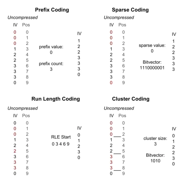
In Figure 2.4 the used techniques for compression in HANA to date are depicted. They are explained in detail in [63].
Prefix coding eliminates the first values of the index vector when they are repeated. In most columns there is no great benefit to use it, except for sorted columns. However, this compression type introduces almost no overhead and does not affect scan performance. Therefore, it is often combined with other techniques.
Sparse coding works by removing the most frequent value IDs from the index vector and managing an additional bit vector, where the positions of removed value IDs are marked. Especially the default value often occurs in columns, therefore this algorithm achieves a good compression ratio in most cases. A disadvantage is that direct access requires the calculation of the value ID’s position in the compressed index vector by building the prefix sum of the bit vector. Depending on the position of the requested value ID this leads to a large overhead compared to the simple access.
Run-length encoding (RLE) (slightly modified version of [32]) compresses sequences of repeating value IDs by only storing the first value of every sequence in the index vector and the start of each sequence in another vector, which can also be bit-compressed. While this may achieve good compression ratios for columns, where values are clustered, there is the possibility that the compressed structure may need even more memory than the uncompressed index vector. Single access to a value ID at a given position requires a binary search in the vector that holds the starting positions and can therefore be expensive.
For cluster coding the index vector is logically split into clusters with a fixed number of value IDs. If one partition holds only equal value IDs, it is compressed to a single value ID. A bit vector stores whether the partition is compressed or not. Similar to RLE this achieves good ratios for clustered values, but the compression is limited by the chosen cluster size. Like with sparse coding a single lookup requires the calculation of the prefix sum for the bit vector and can therefore be expensive. Cluster coding can
Prefix Coding
Run Length Coding 0 0 0 1 2 2 3 3 3 0 Uncompressed 0 1 2 3 4 5 6 7 8 9 Pos IV 1 2 2 3 3 3 0 prefix value: 0 prefix count: 3 IV 0 1 2 3 0 0 3 4 6 9 IV RLE Start Sparse Coding 1 2 2 3 3 3 IV sparse value: 0 Bitvector: 1110000001 Cluster Coding 0 0 0 1 2 2 3 3 3 0 Uncompressed 0 1 2 3 4 5 6 7 8 9 Pos IV 0 0 0 1 2 2 3 3 3 0 Uncompressed 0 1 2 3 4 5 6 7 8 9 Pos IV 0 0 0 1 2 2 3 3 3 0 Uncompressed 0 1 2 3 4 5 6 7 8 9 Pos IV 0 1 2 2 3 0 IV cluster size: 3 Bitvector: 1010
2.2. Main Memory DBMS for a Mixed Workload
be extended toindirect coding by creating a dictionary for a cluster that contains more than one value ID.
Except for prefix compression the direct access to the value ID at a given position gets more expensive the larger the index vector gets. To limit the time needed for such an access, every compression is applied to blocks of values with a fixed size. This way every single lookup requires to calculate the right block number and the access to the structure that stores the compression technique for this block. Afterwards, the block needs to be de-compressed to access the value. The block-wise approach also has the advantage that the best compression algorithm can be chosen for parts of the index vector. Overall this gives a better compression ratio than using one technique for the complete column [63]. Re-Ordering Columns for Better Compression Ratios
All compression techniques shown in the last section do work best for columns that are sorted by the frequency of their value IDs. Especially having the most frequent value ID on top is the best situation in every case, because we can combine all techniques with prefix-coding (of course this is not necessary for RLE). Fortunately, relations do not guarantee any order. Therefore, HANA is free to re-arrange the rows to gain better performance or a smaller memory footprint. Of course, the columns cannot be sorted independently since this would require to map the row number to the position of a value ID. In most cases this would be more expensive (in terms of memory footprint and compression) than having no LWC at all. Hence, the system has to determine which column it sorts for a good performance. Finding the optimal solution for this problem is NP-complete [5]. Lemke et al [63] propose greedy heuristics to find a near-optimal solution. The key to finding a good solution is a combination of only considering columns with small dictionaries and applying the compression techniques to samples of each of these columns.
Compression of String Dictionaries
In typical business scenarios up to 50% of the total databases size are the dictionaries of string columns [87]. In many cases the largest of these dictionaries are the ones that are accesses rarely. In the TPC-H benchmark the comment column of the lineitem table is a typical example [100]. While it is the largest of all columns—uncompressed it is one fourth of the whole database size—there is no query that accesses it. The comment column of the orders table, one eighth of the total, is accessed in one of the 22 queries of the benchmark. The compression of these dictionaries is therefore essential to bring the memory footprint down, while there is no impact on the performance in many cases. Hence, in contrast to index vectors, it can also make sense to use heavy-weight compression on some string dictionaries. But the candidates have to be carefully chosen, since access to certain dictionaries may be performance critical. Ratsch [87] evaluates known compression schemes for string dictionaries in HANA and compares there suitability for common benchmarks. He achieves compression rates between 30% and 50% without a significant impact on the scan-performance. However, the time
needed for initially compressing the dictionaries has to be considered as well. The work shows that automatically determining the right scheme is a complicated task and cannot be done without access statistics and sample queries on the compressed data.
2.2.4. Main and Delta Storage
Although the compression techniques presented in the last section have different char-acteristics in terms of compression ratios, scan-, and single-lookup-performance, they have one thing in common: they have a noticeable impact on the write-performance. In many cases the update of a single value triggers the de- and re-compression of the whole structure that holds the column. The insertion of one row into a large table might take seconds, especially with all the algorithms that are executed to evaluate the optimal compression scheme for parts of the table. This therefore contradicts the original goal of building HANA as a MMDBMS to support mixed-workloads.
Since column stores have a poor write performance in general because of the memory layout, this is a common problem. The general idea is to buffer updates in a secondary data structure, while keeping the main storage static. C-Store [98], for instance, differ-entiates betweenRead-optimized Store (RS)and Writeable Store (WS) [94]. A so called Tuple Mover transfers data in batches from WS to RS.
HANA’s update buffer, called Delta Storage, is optimized to keep read- and write-performance in balance. It stores data in columns just like the main storage, but because it usually holds less data than the main storage, none of the compression techniques, except for dictionary encoding, are used. The delta dictionary is independent of the main dictionary, i.e., values may appear in both dictionaries with different value IDs. In consequence a insertion operation only triggers a lookup in the delta dictionary. In case the value is already there, the value ID is inserted into the column. If the value is not in the column, it is inserted and a new value ID is assigned. While the main dictionary is stored as a sorted array, where the value ID is the position of a value inside the array, the delta dictionary has to use a structure which consists of two parts to provide fast look-ups and insertions. First, values are stored in an array in order of their insertions. The value ID is the position of the of the value within the array. However, finding the value ID belonging to a value takesO(n) operations. Therefore, values are also inserted in a B+-Tree, where they are used as key and the value ID is the (tree-)value. This way, the value ID belonging to a value can be found withO(logn) operations. Insertions have the same complexity.
HANA uses an insert-only approach, i.e., update operations delete the old entry and insert a new one. Because removing the row from main storage immediately would be expensive, it is marked invalid in a special bit-vector instead and finally removed when the delta is merged into the main storage. HANA also supports temporal data, then the bit-vector is replace with two time stamps that mark the time range for which the entry was valid [55].
With the delta approach the main storage can be optimized solely for reading and it can be stored on HDDs as is to guarantee durability. In contrast the delta storage is kept only in main memory, but operations are logged to disk. In case of a a system
2.3. Related Work: Using Co-processors in a DBMS
failure, the main storage can simply be loaded and the delta log has to be replayed to return to the last commited state. Of course data has to be moved from delta buffer to main storage at some point in time. This process—called Delta Merge—creates a new main dictionary with entries from the old main and delta dictionary. Afterwards all value IDs have to be adjusted to the new dictionary. This can be done without look-ups in the new dictionary by creating a mapping from old to new IDs while merging the dictionaries. During the whole operation all write transactions are redirected to a new delta buffer, read transaction have to access the old main and delta as well as the new delta storage. Except for the short time, when the new delta and main are activated, there is no locking required. In Section 4.3 we take a closer look at the creation of the new dictionary.
2.3. Related Work: Using Co-processors in a DBMS
Before we focus on GPUs for the remainder of this thesis, we take a look at related work that concentrates on other available co-processors in the context of DBMS.
FPGAs are versatile vector processors that provide a high throughput. M¨uller and Teubner provide an overview of how and where FPGAs can be used to speed up DBMS in [70]. One of there core messages is that an FPGA can speed up certain operations but should—like the GPU—be used as a co-processor next to the CPU. In [97] the same authors present a concrete use case: doing a stream join on the FPGA.
The stream join was also evaluated on the cell processor in [29, 28]. However, the cell processor is not a typical co-processor but a heterogeneous platform that provides different types of processing units, the PowerPC Processing Element (PPE) and 8 Synergistic Processing Elements (SPEs). The PPE is similar to a typical CPU core, while the SPEs work together like a vector machine. The co-processing concept is inherent in this architecture, because the developer has to decide which processing unit to use for every algorithm. We will face similar challenges in the future with heterogeneous architectures that provide CPU and GPU on the same chip. The same authors also published work about sorting on the cell processor [27].
Recently Intel announced its own co-processor: the Xeon Phi, also called Many In-tegrated Core (MIC), which is a decendant of Larrabee [91]. For the Xeon Phi, Intel adapted an older processor architecture and inter-connected a few dozen cores with a fast memory bus. The architecture focuses on parallel thread execution and SIMD in-structions with wider registers than Xeon processors. It still supports x86 inin-structions, so a lot of software can be ported by re-compiling it. However, to gain performance algorithms have to be adjusted or re-written to support a higher number of threads and vector-processing. Intel published a few insights on the architecture on the use case of sorting in [71]. In 2013 the Xeon Phi also started supporting OpenCL. Therefore, it should be possible to use algorithms written for the GPU. Teodoro et al. compared the performance of GPU, CPU and Xeon Phi in [96].
In a typical computer system there are other co-processors next to the GPU that can be used for general purpose calculations. Gold et al. showed that even a network
3. GPUs as Co-Processors
In the last decade GPUs became more and more popular for general purpose computa-tions that are not only related to graphic’s processing. While there are lots of tasks from different fields ported to the GPU [82], the best known and maybe most successful one is password cracking. With the help of commodity hardware in form of graphic cards it became possible for almost everyone to guess passwords in seconds instead of hours or even days [51]. This shows that the GPU has an immense potential to speed up com-putations. Additionally, it seems that the GPU will be integrated directly into almost every commercial CPU in the future. Therefore, we think that it is the most important co-processor architecture at the moment and concentrate on GPUs for general purpose calculations for the remainder of the thesis.
GPUs use a different architecture than CPUs to process data in a parallel manner. There are similarities with other co-processors, such as FPGAs and Intel’s recently released architecture Xeon Phi. While CPUs use a low number of powerful cores with features such as branch prediction and out-of-order-processing, FPGAs, GPUs, and Xeon Phis consist of dozens to hundreds of weak processing units, which have to be used in parallel to achieve good (or even acceptable) performance. Therefore most of the findings in this thesis also apply to other co-processors, especially if they can be programmed with the OpenCL framework.
We describe the key aspects of the GPU’s architecture and compare it to the CPU in Section 3.1. The main problem when offloading calculations to an external co-processor is, that it has to communicate with the CPU to get input data and transfer the results back. We discuss the influence of this bottleneck in Section 3.2. To interact with GPUs developers have the choice between direct programming and the usage of libraries that transparently process data on the GPU. OpenCL1and CUDA2are the two most common frameworks to program GPUs directly. There characteristics and available libraries for the GPU are described in Section 3.3. The main part of this chapter in Section 3.4 focuses on different micro benchmarks to show the strong- and weak-points of the GPU. Based on the characteristics we can derive from these benchmarks we draw a conclusion and outline the remainder of the thesis in Section 3.5.
3.1. SIMD Processing and Beyond
Flynn specified four classes of machine operations [24], which are still used today to differentiate between parallel processor architectures. We introduce the taxonomy in
1http://www.khronos.org/opencl/ 2
Subsection 3.1.1. However, neither CPU nor GPU fall into only one category. Both architectures are mixed, but have a tendency. In Section 3.1.2 we discuss this further.
3.1.1. Flynn’s Taxonomy
The four classes of Flynn’s Taxonomy are shown in Figure 3.1:
Single Instruction Single Data (SISD) describes a processor with one processing unit that works on one data stream. In this work we often refer to this as sequential process-ing. Before the first SIMD instruction sets, e.g., MMX, 3DNow!, and Streaming SIMD Extensions (SSE), were introduced, single core processors were working in a pure SISD manner.
Single Instruction, Multiple Data (SIMD) means that a number of processing units are executing the same statements on different data streams. In the 1970s vector pro-cessors were working like that. Today most propro-cessors (CPUs and GPUs) have parts that work in a SIMD fashion.
Multiple Instruction, Single Data (MISD) requires a number of processing units to do different instructions on the same data stream. This processing model can be used for fault tolerance in critical system. Three or more processors do the same operation and there results are compared.
Multiple Instruction, Multiple Data (MIMD) describes processing units that can in-dependently work on different data streams. In contrast to just using multiple SISD processors this approach allows to share resources that are not needed exclusively, e.g., the memory bus or caches.
Multi-Core CPUs can be roughly classified as MIMD and GPUs as SIMD architec-tures. However, both have aspects of the other architecture. The MIMD-nature of mod-ern multi-core CPUs is obvious to most developers. Threads can work independently on different algorithms and data segments in at the same time. However, with instruction sets such as SSE and Advanced Vector Extensions (AVX) it is also possible to parallelize execution within one thread, e.g., building the sum of multiple integers with one instruc-tion. This SIMD aspect of the CPU is almost hidden, because in most cases this type of processing happens without the developer’s explicit interference. The compiler analyses the code and uses SIMD-instructions automatically. Nevertheless these instructions can be used explicitly and the benefit may be dramatic in some cases [104, 103].
Nowadays, no (pure) SISD processors can be found in server, desktop, or mobile computers. Even single-core CPUs usually have more than one processing unit to execute SIMD instructions. Multi-Core CPUs and GPUs, as well as Xeon Phis, are a mixture of SIMD and MIMD processors. However, the SIMD aspect of GPUs is important because of the high number of cores that work in single lock step mode. On the CPU SIMD is available in form of instructions, which are used by modern compilers automatically.
3.1. SIMD Processing and Beyond Instructions Data PU Instructions Data PU PU PU PU Instructions Data PU PU PU PU Instructions Data PU PU PU PU SISD MISD SIMD MIMD
Figure 3.1.: Flynn’s taxonomy
3.1.2. Hierarchy of Parallelism—the GPU Architecture
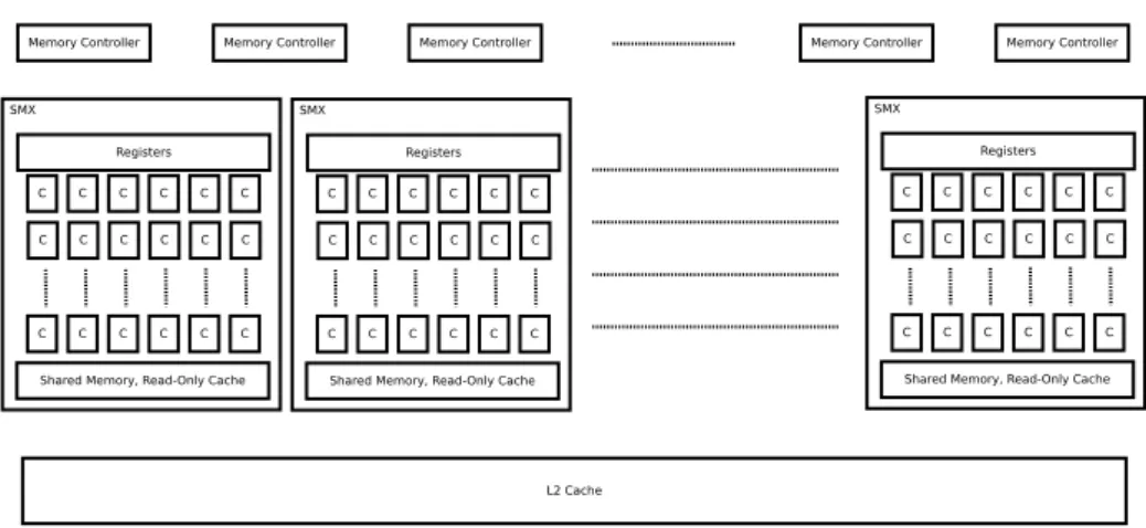
While GPUs are often referred to as SIMD processors, its architecture is actually MIMD-SIMD-hybrid. Figure 3.2 depicts the simplified NVIDIA Kepler GK110 architecture, which we explain exemplary in this section. We use the NVIDIA terminology for the description, the concepts in principle are similar to hardware of other vendors.
The 2880 processing cores on the GPU are grouped in 15 Streaming Multi Processors (SMXs). 192 cores on each SMX share a single instruction cache, 4 schedulers, and a large register file. They are interconnected with a fast network, which among other thins provides (limited) access to registers of other cores. Hence, all the cores of one SMX are tightly coupled and designed for SIMD processing. Consequently, threads on the cores are executed in groups of 32. Such a group is called awarp and is able to execute only 2 different instructions per cycle, i.e., in every case at least 16 cores execute exactly the same instruction, they run in single-lock-step mode.
Compared to the internals of a SMX the coupling between different SMXs of a GPU is loose. Threads are scheduled in blocks by the so-called GigaThread engine, there is no global instruction cache, and the cores of different SMXs cannot communicate directly. In consequence, no synchronization between threads of different SMXs is possible. They operate independently and represent the MIMD processing part of the GPU’s architec-ture. Hence, one SMX works similar to a vector machine, but the whole GPU is more like a multi-core vector machine.
C C C C C C
C C C C C C
C C C C C C
Registers
Shared Memory, Read-Only Cache SMX
C C C C C C
C C C C C C
C C C C C C
Registers
Shared Memory, Read-Only Cache SMX
C C C C C C
C C C C C C
C C C C C C
Registers
Shared Memory, Read-Only Cache SMX
L2 Cache Memory Controller
Memory Controller Memory Controller Memory Controller Memory Controller
Figure 3.2.: Simplified architecture of a GPU
The memory hierarchy supports this hybrid processing model. Not only do processing cores of one SMX share a register file, they also have fast access to 64 kB of Shared Memory. This can be configured to either act as L1 cache or as memory for fast data exchange. In each SMX there is additional read-only and texture memory, which is optimized for image processing. Between SMXs there is no other way to share data than using DRAM. While DRAM on the GPU usually has a much higher bandwidth than the RAM used for CPUs it also has a much higher latency (a few hundred cycles in modern GPUs). In contrast to CPU processing, where thread/context-switches wipe registers, on the GPU every threads keeps its own registers in the register file. Therefore, it is possible to load one warp’s data from DRAM to the registers while other warps are running. This method of overlapping is the key for good performance on the GPU, but makes it necessary to execute much more threads than cores. Otherwise, most threads wait for DRAM, while only a few can be executed. Depending on the scenario this under-utilization happens when there are less than be 10 to 100 threads per core. Modern GPUs address the problem of the DRAM’s high latency by providing one L2 cache for all SMXs that operates automatically—similar to the L2 cache on CPUs. On Kepler it has a size of 1538 kB. Since memory is always accessed by a half-warp, the GPU is optimized forcoalesced access. Agian this is simplified but it means that consecutive threads should access consecutive memory addresses. More information about this topic and details about Kepler can be found in the best practices guide for CUDA [73] and the architecture whitepaper [77].
3.1.3. Programming Model for GPU Parallelsim
The hybrid architecture of multiple SIMD-processors requires a different way of applying parallel aspects to algorithms. With threads as parallel execution paths on the one hand the differences in SIMD and MIMD cannot be expressed. Simple parallel instruction and paradigms such as OpenMP’sparallel for on the other hand are not flexible enough; the same counts for special SIMD instructions such as Intel’s SSE or AVX. Therefore,
3.2. Communication between CPU and GPU
a model of workgroups and threads to differentiate between the MIMD and the SIMD aspects was introduced. Both, OpenCL and CUDA are implementations of this model, we take a look at their differences in Section 3.3.
When you launch a function on the GPU, it will start a fixed number of workgroups and each workgroup consists of a fixed number of threads. Although this is not exact, it makes sense to imagine that one SMX executes a workgroup with all its cores. Workgroups run independent of each other and can only be synchronized by ending the function and starting a new one. In contrast to the workgroups themselves their threads can be easily synchronized and are able to exchange data via a small block of shared memory, which can be accessed with a very low latency (a few cycles depending on the hardware). The number of threads per workgroup is usually called workgroup size. Since at least one warp is always executed, it makes sense to choose a multiple of 32 as workgroup size. In some situations it is useful to know that a group of 32 threads needs no explicit synchronization, but in most cases hardware and compiler take care of an optimization like this. Hence, threads of one workgroup should be handled as if they run in lock-step mode, i.e., every thread executes the same instruction on data in its registers in one cylce.
3.2. Communication between CPU and GPU
The way of communication between the CPU and the GPU depends on the GPU’s type. In general, we can differentiate between three classes of co-processors by looking at their integration into the computer’s CPU.
1. Co-processors such as most graphic cards today are connected via the PCI-Express (PCIe) bus, i.e., data has to be transferred to the graphic cards memory, where the GPU can access it. For data-intensive tasks this is the bottleneck [37]. Intel’s XeonPhi and FPGAs are also usually connected via PCIe.
2. The second class of co-processors is tightly integrated into the system bus. The GPU part of AMD’s APUs fits into that category. It still operates on its own but it shares memory with the CPU [17]. Therefore data can be transferred much faster. 3. Modern CPUs consist of a collection of co-processors of the third class. The FPU for instance is now integrated and has special registers on the CPU. Cryptographic processors also fall into this category. There are special instructions for these co-processors in the CPU’s set. A software developer usually does not explicitly use the instructions since the compiler or interpreter automatically does that.
In this work we are focusing on the first class of co-processors, also called external co-processors. In Chapter 6 we will address the second class, which is at the moment often referred to as heterogeneous processor architecture.
3.3. Software Frameworks and Libraries
Co-processors for general-purpose calculations require special software to use them. De-velopers have to decide whether they want to use a framework to write low-level-code or libraries that provide functions for a certain domain. When programming for NVidia GPUs, which are used in all experiments in this thesis, one has the choice between us-ing OpenCL and CUDA. The advantage of OpenCL over CUDA is that not only other co-processors but also the CPU is able to execute it. We conducted some experiments that show that we can run OpenCL code developed for the GPU on the CPU without changes (see Section 5.5.3). Although this might be slower than a native parallel CPU implementation, it is still faster than sequential execution. Next to CPUs, other GPU vendors also support OpenCL. AMD even stopped developing Stream, which was their specific framework for General Purpose Graphics Processing Unit (GPGPU) computing. Intel also provides OpenCL for their GPUs and for the Xeon Phi. We expect future de-vices from different vendors to use OpenCL as well, because it is an open specification and many applications already support it.
Both frameworks focus on parallel architectures and are very similar in principle. The code running on the GPU—more general the device—is called kernel and uses the pro-gramming model of workgroups and threads as explained above. OpenCL and CUDA are both dialects of the C programming language. In many cases it is easy to transform code between CUDA-C and OpenCL-C, because it is mostly a matter of translating key-words. For example, synchronizing threads is done by__syncthreads() in CUDA and barrier(CLK_LOCAL_MEM_FENCE)in OpenCL. In general CUDA provides more language features, such as object orientation and templates, as well as more functional features. As long as the missing functional features in OpenCL do not limit the algorithm the run-time of OpenCL and CUDA kernels for the same purpose is comparable in most cases. According to the authors of [53] OpenCL is mostly slower (13% to 63%) on NVidia GPUs, but they found that often there is no difference in performance at all. However, sometimes kernels can be designed in another way with features only available in CUDA, such as Dynamic Parallelism and dynamic memory allocation. The first one allows to spawn kernels from inside other kernels and the synchronization of all threads on the device and the second feature allows developers to allocate memory inside kernels. This opens up new possibilities, which might affect performance as well (see Section 3.4.1).
The conceptional difference between OpenCL and CUDA is the way, kernels are com-piled. CUDA has to be compiled by NVidia’s nvcc and the object files are then linked to the CPU object code. To support future devices the compiler allows to include an intermediate code, called PTX, which is generated by nvcc at compile time and then used to produce the binary code for the specific device by the CUDA run-time. Because OpenCL targets a wider range of devices, it makes no sense to deliver device-specific code and ship it with the binaries in advance. Instead the OpenCL code is compiled at run-time by the driver of the device. In Chapter 5 we use this feature for our query execution framework.
In Section 3.1.2 we already mentioned that there are details about the architecture, that are performance critical when unknown, e.g., coalesced memory access or
under-3.3. Software Frameworks and Libraries
utilization. There are many other pitfalls in GPU-programming, but similar to CPU software there are already libraries that provide optimized algorithms for certain do-mains.
Thrust Similar to the Standard Template Library (STL) in C++ the Thrust library provides basic algorithms to work with vectors of elements. It provides transformations, reductions, and sorting algorithms for all data types available on the GPU.
CUBLAS Algorithms for the domain of linear algebra is available for NVIDIA devices in form of the CUBLAS. As the name suggests the library provides the common Basic Linear Algebra Subprograms (BLAS) interface to handle vectors and matrices. The CUSPARSE library provides similar algorithms for sparse matrices and vectors.
CUFFT The CUFFT library provides the CUDA version of Fourier transforms, which are often needed in signal processing
NPP The NVIDIA Performance Primitives are a library for image and video process-ing. In contrast to the other libraries, where every function spawns at least one kernel, the functions of the NPP can also be called from within kernels.
unified SDK The BLAS and FFT primitves are also available in OpenCL as part of the unified SDK. It also includes the former Media SDK with video pre- and post-processing routines.
Another way to use parallel co-processors without handling the details of the under-lying hardware is OpenACC [79]. With OpenACC developers can use patterns to give the compiler hints on what can be parallelized and executed on the GPU. Listing 3.1 shows code for the matrix multiplication in C with OpenACC. The pragma in line 1 tells the compiler that the following code block should be executed on the co-processor, a and b are input variables, and c has to be copied back to the host after kernel execu-tion. By describing the dependencies between the iterations of a loop, the compiler can decide how to parallelize execution. Loop independent in lines 3 and 5 encourages to distribute the execution over multiple cores while loop seqforces the execution of one loop to one core, because every iteration depends on the previous one.
Listing 3.1: Matrix multiplication in OpenACC 1 # p r a g m a acc k e r n e l s c o p y i n ( a , b ) c o p y ( c ) 2 { 3 # p r a g m a acc l o o p i n d e p e n d e n t 4 for ( i = 0; i < s i z e ; ++ i ) { 5 # p r a g m a acc l o o p i n d e p e n d e n t 6 for ( j = 0; j < s i z e ; ++ j ) { 7 # p r a g m a acc l o o p seq 8 for ( k = 0; k < s i z e ; ++ k ) {
![Table 2.1.: Approximation of latency for memory access (reads) [64, 30, 105]](https://thumb-us.123doks.com/thumbv2/123dok_us/68208.2507851/18.892.186.712.145.317/table-approximation-latency-memory-access-reads.webp)
![Figure 2.1.: Overview of the SAP HANA DB architecture [22]](https://thumb-us.123doks.com/thumbv2/123dok_us/68208.2507851/19.892.133.756.146.405/figure-overview-sap-hana-db-architecture.webp)