Louisiana State University
LSU Digital Commons
LSU Doctoral Dissertations Graduate School
2013
Exploring the Learnability of Numeric Datasets
Di Lin
Louisiana State University and Agricultural and Mechanical College, [email protected]
Follow this and additional works at:https://digitalcommons.lsu.edu/gradschool_dissertations Part of theComputer Sciences Commons
This Dissertation is brought to you for free and open access by the Graduate School at LSU Digital Commons. It has been accepted for inclusion in LSU Doctoral Dissertations by an authorized graduate school editor of LSU Digital Commons. For more information, please [email protected].
Recommended Citation
Lin, Di, "Exploring the Learnability of Numeric Datasets" (2013).LSU Doctoral Dissertations. 1836.
EXPLORING THE LEARNABILITY OF NUMERIC DATASETS
A Dissertation
Submitted to the Graduate Faculty of the Louisiana State University and Agricultural and Mechanical College
in partial fulfillment of the requirements for the degree of
Doctor of Philosophy in
The School of Electrical Engineering and Computer Science Computer Science and Engineering Division
by Di Lin
B.S., FuZhou University, 2003 M.S., Louisiana State University, 2011
Acknowledgements
Over the past six years I have received support and encouragement from a great number of indi-viduals. Dr.Evangelos Triantaphyllou has been a mentor, colleague, and friend. His guidance has made this a thoughtful and rewarding journey. I would like to thank my dissertation committee of Dr.Jian Zhang and Dr. Jianhua Chen, for their support over the past couple years as I moved from an idea to a completed study.
Table of Contents
Acknowledgements . . . ii
Abstract . . . viii
Chapter 1: Introduction . . . 1
Chapter 2: Introduction to Monotonicity . . . 4
2.1 The Monotonic Property in Datasets . . . 4
2.2 Key Definitions Related to Monotonicity . . . 6
2.3 Graphical Representation in Two Dimensions . . . 11
2.4 Data with both Positive and Negative Attributes . . . 12
2.5 Graphical Representation for Datasets With Positive and Negative Attributes . . . . 15
2.6 Types of Pairs of Vectors . . . 17
Chapter 3: The Experimental Design for Binary Datasets . . . 20
3.1 Design Issues of Experiments with Some Artificial Binary Datasets . . . 20
3.2 Generating the Binary Experimental Datasets . . . 21
3.3 Classifiers from WEKA . . . 26
Chapter 4: The Experimental Study . . . 28
4.1 Parameters Used to Describe the Monotone Structure of a Dataset . . . 28
4.2 Experiments with Binary Datasets . . . 31
4.3 Experiments with Some Continuous Datasets . . . 38
Chapter 5: A Meta-Learning Approach . . . 47
5.1 The Motivation of the Meta-Learning Approach . . . 47
5.2 Data Pre-processing . . . 48
5.3 The Pilot Study . . . 50
5.4 The Proposed Approach to Improve Classifications . . . 51
5.5 A Monotonicity-Based Classification Approach . . . 52
Chapter 6: Experiments For Meta-Learning Approach . . . 59
6.1 Some Preliminaries on the Experiments . . . 59
6.2 The Experimental Results . . . 60
6.3 Analysis of the experimental results . . . 72
Chapter 7: Conclusions . . . 79
7.1 An Overview of this Research . . . 79
References . . . 83 Vita . . . 88
List of Tables
2.1 An example of a purely monotonic datasetDin{0,1}4. . . . 8
2.2 An example of a non-purely monotonic datasetDin{0,1}5. . . . 10
2.3 An example of a purely monotonic binary training dataset when positive/negative attributes are taken into consideration. . . 16
2.4 An example of a non-purely monotonic binary training dataset when positive/negative attributes are taken into consideration. . . 16
3.1 The number of AMP2 and CMP pairs in the completen-attribute binary datasets that are generated by the approach dessribed in Section 3.2.3. . . 24
4.1 The seven monotonic characteristics of the numeric datasets. . . 29
4.2 The regression models generated for different dimensions of artificial binary datasets. 33 4.3 Details of the regression models listed in Table 4.2. . . 33
4.4 The information of the datasets listed in Table 4.5. . . 37
4.5 The regression models generated for some real-life binary datasets. . . 37
4.6 Experimental results from the real-life binary datasets listed in Table 4.5. . . 38
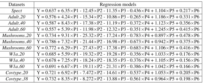
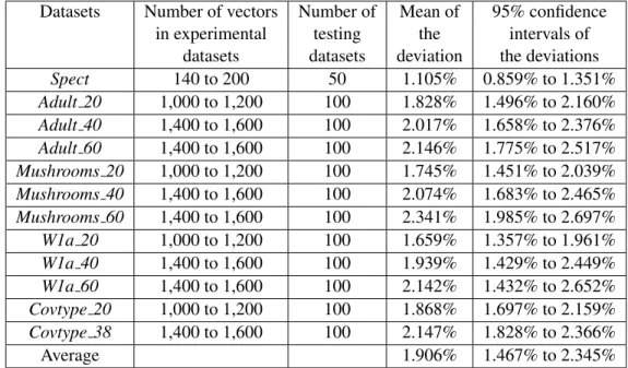
4.7 Regression models generate from some real-life continuous datasets. . . 41
4.8 Experimental results from real-life continuous datasets listed in Table 4.7. . . 42
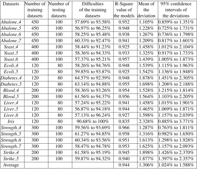
4.9 Some characteristics of the regression models generated independently of the test-ing data. The actual regression models are shown in Table 4.10. . . 44
4.10 Regression models for datasets listed in Table 4.9. . . 45
5.1 Some Characteristics of the Experimental Datasets. . . 50
6.1 Some experimental results when analyzed theAbalonedatasets. . . 63
6.3 Some experimental results when analyzed theYeastdatasets. . . 65
6.4 Some experimental results when analyzed theCar evaluationdatasets. . . 66
6.5 Some experimental results when analyzed theAuto MPGdatasets. . . 67
6.6 Some experimental results when analyzed theMammodatasets. . . 68
6.7 Some experimental results when the 5-attribute artificial datasets were analyzed. . . 69
6.8 Some experimental results when the 6-attribute and 7-attribute artificial datasets were analyzed. . . 70
6.9 Some details of experiments when usingDecision Tree(J48) as the base classifier. . 74
6.10 Some details of experiments when using Artificial Neural Network as the base classifier. . . 74
6.11 Some details of experiments when usingADTreeas the base classifier. . . 75
6.12 Some details of experiments when usingSupport Vector Machineas the base clas-sifier. . . 75
6.13 The details of the linear regression models for the experimental results listed in Table 6.9. . . 76
6.14 The details of the linear regression models for the experimental results listed in Table 6.10. . . 77
6.15 The details of the linear regression models for the experimental results listed in Table 6.11. . . 77
6.16 The details of the linear regression models for the experimental results listed in Table 6.12. . . 77
List of Figures
2.1 The poset for the dataset in Table 2.1 and its border points. . . 11
2.2 The poset for the dataset in Table 2.2 and its border points. . . 11
2.3 The complete poset whenn=4,x=2, andy=2. . . 15
2.4 The poset for the dataset listed in Table 2.3 and its border points. . . 16
2.5 The poset for the dataset listed in Table 2.4 and its border points. . . 16
2.6 Some examples of different types of monotonically related pairs. . . 19
4.1 Relationships between average accuracy and some monotonic features for binary datasets whenn= 8. They may have different positive/negative attributes. . . 29
4.2 The R-Square values of the models generated from artificial binary datasets with different dimensions. . . 32
4.3 The R-Square values of the models generated from continuous experimental groups with different levels of monotonicity. . . 40
5.1 Different cases of scenarios of the monotonicity observed in functions. . . 48
5.2 The relationship between the difficulty of the datasets andPkeyvalues. . . 51
Abstract
When doing classification, it has often been observed that datasets may exhibit different levels of difficulty with respect to how accurately they can be classified. That is, there are some datasets which can be classified very accurately by many classification algorithms, and there also exist some other datasets that no classifier can classify them with high accuracy. Based on this ob-servation, we try to address the following problems: a)what are the factors that make a dataset easy or difficult to be accurately classified? b) how to use such factors to predict the difficul-ties of unclassified datasets? and c) how to use such factors to improve classification. It turns out that the monotonic features of the datasets, along with some other closely related structural prop-erties, play an important role in determining how difficult datasets can be accurately classified. More importantly, datasets which are comprised of highly monotonic data, can usually be classi-fied more accurately than datasets with low monotonically distributed data. By further exploring these monotonicity based properties, we observed that datasets can always be decomposed into a family of subsets while each of them is highly monotonic locally. Moreover, it is proposed in this dissertation a methodology to use the classification models inferred from the smaller but highly monotonic subsets to construct a highly accurate classification model for the original dataset. Two groups of experiments were implemented in this dissertation. The first group of experiments were performed to discover the relationships between the data difficulty and data monotonic properties, and represent such relationships in regression models. Such models were later used to predict the classification difficulty of unclassified datasets. It seems that in more than 95% of the predictions, the deviations between the predicted value and the real difficulty are smaller than 2.4%. The sec-ond group of experiments focused on the performance of the proposed meta-learning approach. According to the experimental results, the proposed approach can consistently achieve significant improvements.
Keywords:Data mining, classification models, monotonic property, decomposition approaches, binary datasets, monotonicity, monotonic characteristics, monotone functions, regression models, data analysis.
Chapter 1
Introduction
How to efficiently and effectively analyze datasets of data grouped into classes has always been a crucial challenge in data mining research. Currently, there are numerous algorithms in use which infer classification models from such datasets. Next, these classification models may be used to infer the class values of new data points for which the class values are unknown. Such algorithms infer classification models by implementing various, and often times, quite diverse strategies. Ex-amples include support vector machines (SVMs) [39, 7, 9], neural networks [30, 40, 47], decision trees [6, 36, 1], and logic-based approaches [43, 26, 24, 17, 13], just to name a few.
An interesting observation derived from numerous studies (see, for instance, [39, 24, 40]) is that often times some datasets may be analyzed very accurately by a wide spectrum of classifiers while other datasets may not be analyzed as easily. In other words, it seems like there are “easy” datasets, “difficult” datasets and datasets of intermediate degrees of difficulty when one is interested on how easily they can be analyzed accurately by classifiers. Therefore, in this study the difficulty of a dataset is evaluated by the average classification accuracy when it is analyzed by various classifiers, the lower the accuracy, the more difficult the dataset is. Furthermore, in this dissertation this property is also defined as thelearnabilityof datasets.
This study focuses on this very issue. That is, the main research question studied here is how one can predict whether a given dataset would be analyzed accurately by a wide spectrum of clas-sifiers. A theoretical analysis and some computational results provided in the following sections indicate that a property in data known as the monotonicity property plays a central role in deter-mining whether a given dataset is “easy,” “difficult” or of intermediate degree of difficulty when one focuses on the above classification task. More importantly, it is also observed that some
mono-tonic based properties are strongly related to their monomono-tonic property, and which could be used to accurately predict the learnability of datasets.
At present, if one wishes to determine whether a given dataset can be easily classified with high accuracy, then that dataset has to be analyzed by many classifiers. The inferred models are evaluated in terms of how accurate they are when they are fed with new data points of hidden class values. However, such an approach may have a number of weaknesses. First, it might be a time consuming approach, as many different classifiers need to be employed. Second, even if the results are highly conclusive at the end of such a tedious study, one still does not really know what makes a dataset easy or difficult to be classified accurately. Furthermore, if a dataset is deemed as a difficult one because a number of classifiers have difficulty inferring accurate models, does it mean that this dataset is truly a hard one? After all, which classifiers should be used in such studies? How many of them? Currently, such questions cannot be answered objectively.
Therefore, a theoretical understanding of what makes a dataset easy or hard, based on its struc-ture alone, is of paramount importance in this area of data mining research. Furthermore, if one knows that a given dataset is a hard one because of properties pertinent to this dataset, then a new classifier which outperforms existing ones even by a few percentage points, might be considered as an important contribution. On the other hand, if a new classifier performs only slightly better when dealing with easy datasets, then such news might not be as important.
It is observed that when datasets are comprised of highly monotonic data, then they can be classified accurately by most methods while datasets that are not comprised of highly monotonic data, tend to be more difficult to be accurately analyzed by classifiers. Then the challenge becomes what happens if a given dataset does not exhibit strong monotonicity, is there any way to make it easier to be accurately classified, perhaps after some data manipulations? The present dissertation provides an answer to this very important question.
In summary, our research is concerned with the following issues: what are the factors that impact the difficulty of datasets, how to derive such factors, how to use them to evaluate the difficulty of
the datasets objectively, under what conditions is the proposed approach applicable, and more importantly, how to use the previous results on poorly monotonic data, such that the classification accuracies can be improved.
The rest of the dissertation is organized as follows. Section 2 introduces the notion of mono-tonicity and also provides the definitions of the monotonic features considered in this study. The third section illustrates how some binary datasets were generated for this study. The fourth section demonstrates how the monotonic characteristics of datasets can be used to predict their classifica-tion difficulty. This is done for some binary datasets and some continuous datasets. The fifth secclassifica-tion provides a way to pre-process the raw data to make them easier to accurately classify, while the sixth section shows a meta-learning approach to improve the classification on any numeric datasets. Finally, this dissertation ends with the main conclusions of our study.
Chapter 2
Introduction to Monotonicity
2.1
The Monotonic Property in Datasets
Because monotonicity plays a central role in the developments described in our research, this section presents a brief discussion of the notion of monotonicity and some key developments in this area. This discussion on monotonicity is important even for datasets that are not purely monotonic. This is true because as it is explained later, even when monotonicity is partially present in a dataset, then one may still be able to reach certain important conclusions when the learnability of that dataset is concerned.
For a simple and intuitive illustration of what is monotonicity in data, let us consider the follow-ing hypothetical situation. Suppose an analyst is interested in studyfollow-ing how a personal computer (PC) may crash under various software application loading scenarios. This analyst has observed that when certain software applications are loaded simultaneously, then the PC may crash. As there arenpossible applications to be loaded, the state of the PC may be represented in terms of binary vectors inndimensions. The analyst has observed that under certain loading scenarios the PC may crash (class value 1), while under some other loading scenarios the PC may not crash (class value 0).
For instance, if a word processor, a photo editor and a video editor are loaded simultaneously, then the PC may crash (class value 1). Suppose that forn=10 (i.e., there are up to 10 applications to be loaded), the previous scenario is represented by the following binary vector:V1= (0100101000), where the three 1s represent the loading of the previous three applications, respectively. Then one may argue, that if the previous three applications have been loaded and then two more are loaded in addition (such as the ones represented by the following vector:U1 = (0110101010)), then the PC may crash as well (class value 1).
This is reasonable to assume because the new state of the PC describes a situation that is even more strenuous than the previous one, under which nevertheless the PC would crash. Please also observe that for these two vectors the following is true:U1>V1. In a similar manner, if the PC does not crash under a given software loading scenario, say, the one represented by the vectorV2 = (0100001110), then most likely it will not crash under the loading scenarioU2= (0100001010), which represents a lighter case. In other words, if a Boolean function f exhibits the following property: f(U)≥ f(V), for any two vectorsUandV such thatU≥V, then we say that the function
f is monotonically increasing.
More formally, let{0,1}n denote the binary space defined onnBoolean attributes. ABoolean
function defined on this space is a mapping from {0,1}n into {0,1}. Suppose that two binary vectorsU andV from{0,1}nare given whereU =(u
1,u2,u3, . . . ,un)andV =(v1,v2,v3, . . . ,vn), andui,vi = 0 or 1 for anyi = 1,2,3,. . .,n. Then, there are three possible cases as described in the following definitions.
Definition 2.1:A binary vector U∈ {0,1}nis said to begreater than or equal toanother vector V ∈ {0,1}n, denoted as U≥V , if and only if (iff) ui≥vi, for i=1,2,3, . . . ,n, where ui(vi)denotes the ith element of vector U(V).
Definition 2.2:A binary vector U ∈ {0,1}n is said to be less than or equal toanother vector V ∈ {0,1}n, denoted as U ≤V , iff u
i≤vi, for i=1,2,3, . . . ,n, where ui(vi)denotes the ithelement of vector U(V).
Definition 2.3:Given two vectors U,V ∈ {0,1}n, they are said to beunrelatedto each other iff neither one is greater than or equal to the other. Otherwise, they are calledrelated.
If a vectorU is greater than another vectorV, then one can also say that vectorU proceeds vectorV, or in other words, thatvectorV follows vectorU. For some illustrative examples of the above, consider the four vectors in{0,1}4defined as follows:V = (1011),W = (0011),P= (0001) and Q = (1001). Then according to the previous definitions, it follows thatV >W andW >P,
and it is easy to getV >P as well. Moreover, the vectorsW andQ are unrelated. The following definition provides the notion of monotone Boolean functions formally.
Definition 2.4:A Boolean function f defined on{0,1}n, is calledmonotonically increasingiff f(U)≥ f(V) for all U,V ∈ {0,1}n, and U ≥V . If f(U)≤ f(V) for all pairs of vectors U,V ∈
{0,1}nsuch that U≥V , then such Boolean function is calledmonotonically decreasing.
In this dissertation when we say monotone Boolean function we will mean an increasing one unless it is otherwise specified. The first known study on monotonicity is due to Dedekind [14]. Other early studies are due to Church [11] and Ward [45] where they studied the number of all Boolean monotone functions for dimensionsn=1,2,3, . . . ,7. An interesting development is due to Hansel [23] who introduced the notion of Hansel chains. Some early learning complexity issues for inferring monotone Boolean functions were studied in [38, 22, 19, 28, 3, 32]. More recent studies on learning monotone Boolean functions from training data can be found in [41, 43].
2.2
Key Definitions Related to Monotonicity
Given a monotone Boolean function f from {0,1}n into {0,1}, some vectors in {0,1}n play a critical role in defining this function f. These are what is known as upper zero and lower unit vectors [23, 41, 43]:
Definition 2.5:A vector V∗is called alower unit of a monotone Boolean function f iff f(V∗) = 1 and f(V)< f(V∗), for any vector V <V∗.
Definition 2.6:A vector V∗is called anupper zero of a monotone Boolean function f iff f(V∗) = 0 and f(V)> f(V∗), for any vector V >V∗.
Definition 2.7:Given a monotone Boolean function f the union of the set of the lower units with the set of the upper zeros is the set of itsborder vectors.
For any monotone Boolean function f, the set of all lower units and the set of all upper zeros are unique, and either one of these two sets uniquely identifies f [41].
2.2.1
Purely Monotonic Binary Datasets
Next, it is assumed that given is a binary dataset, sayD, comprised of two mutually exclusive and exhaustive subsets of binary vectors classified by some monotone Boolean function f. The analyst may or may not know the definition of this function f. The first subset, denoted asD+, has all the vectors classified as positive, while the second subset, denoted asD−, has all the vectors classified as negative. Obviously,D=D+∪D−.
Definition 2.8:A binary dataset D is apurely monotonic binary dataset iff any positive vector V ∈D+ is either greater than any negative vector U ∈D− or the vectors V and U are unrelated.
If the condition described in the previous definition is not satisfied, the dataset is called a non-purely monotonic binary dataset. Next, the previous concepts of upper zeros, lower units, and border points of monotone Boolean functions can be easily adapted in the context of a purely monotonic binary datasetD. This is accomplished in terms of the following definitions:
Definition 2.9:Given a purely monotonic binary dataset D, a vector V∗∈D+ is called alower unit of the datasetD iff for any V ∈D+, V∗<V or the vectors V∗and V are unrelated.
Definition 2.10: Given a purely monotonic binary dataset D, a vector V∗ ∈D− is called an
upper zero of the datasetD iff for any V ∈D−, V∗>V or the vectors V∗and V are unrelated.
Definition 2.11: Given a purely monotonic binary dataset D, the union of the set of its lower units with the set of its upper zeros is the set of itsborder points.
The previous concepts can be easily extended to functions and datasets that are not binary. This can happen if the attributes take on ordinal values and thus one can compare vectors as was the case with only binary attributes. Algorithm 1 can be used to identify the border points of a purely monotonic dataset (no necessarily only binary). As illustrative examples of these concepts, consider the dataset in{0,1}4depicted in Table 2.1. The lower units ofDare the vectors:{(1100), (1010)}, while the upper zeros ofDare the vectors:{(0110), (1001), (0101)}. The set of its border points is the union of the previous two sets.
TABLE 2.1: An example of a purely monotonic datasetDin{0,1}4. Positive vectors (1111), (1110), (1101), (1011), (1100), (1010) Negative vectors (0110), (1001), (0101), (0100), (0001), (0000)
Algorithm 1:Find all the border points in a purely monotonic datasetD.
Input :E+,E−; /*Two mutually exclusive sets of positive and negative vectors inD, respectively.*/
Output: LU,UZ; /*Two sets of the lower units and the upper zeros, respectively.*/
1 foreach e+i ∈E+ do 2 foreach e+j ∈E+do 3 ife+j >e+i then 4 Removee+j fromE+; 5 end 6 end 7 end 8 foreach e−i ∈E− do 9 foreach e−j ∈E−do 10 ife−j <e−i then 11 Removee−j fromE−; 12 end 13 end 14 end 15 LU ←E+ andU Z←E−; 16 Return LU, UZ;
2.2.2
Non-purely Monotonic Binary Datasets
Some real-life datasets, however, may not be purely monotonic. That is, in such datasets one may encounter positive vectors which may be less than some negative vectors. When this happens, then the previous defined concepts should be modified to become the extended lower units, the extended upper zeros, and the extended border points of the dataset.
To be more specific, if a binary dataset is not purely monotonic then it can be decomposed into groups of vectors such that within each pair of groups the monotonic property holds locally. In particular, such dataset can be divided into several unique class groups. Each group contains the vectors with same class value, while the class values between adjacent groups are different. Moreover, for any two groups of such vectors with different class values, all the vectors in one
group precede or are unrelated to the vectors in the other group. In this way, any two groups of vectors of opposite class values can comprise a purely monotonic binary dataset.
Suppose that given is a binary dataset D which is not purely monotonic. Then, its sub-groups can be derived as follows:
1. Find out all the positive vectors inDwhich precede or are unrelated to all negative vectors. Next, they are removed fromDto form a positive sub-group.
2. From the remaining vectors, find out all the negative vectors which precede or are unrelated to the rest of the positive vectors. Next, they are removed from Dto form a negative sub-group.
3. Repeat steps (1) and (2) until the datasetDbecomes empty.
Based on such unique class groups, the concept of extended border points can be defined as follows:
Definition 2.12:Given a positive sub-group G, a vector V∗∈G is called anextended lower unit of the sub-groupG iff for any V ∈G, then V∗<V or the vectors V∗and V are unrelated.
Definition 2.13:Given a negative sub-group G, a vector V∗∈G is called an extended upper zero of the sub-groupG iff for any V ∈G, then V∗>V or the vectors V∗and V are unrelated.
Definition 2.14: Given a non-purely monotonic binary dataset D, the union of the set of its extended lower units with the set of its extended upper zeros forms the set of itsextended border points.
Once the sub-groups are determined as above, the border points of each sub-group can be de-termined by implementing Algorithm 1 within each sub-group. As was the case with the deter-mination of the (regular) lower unit and upper zero vectors, an algorithm can be easily designed to determine the extended lower unit and extended upper zero vectors. Algorithm 2 shows such an approach with a time complexity of O(m2), where mis the number of vectors in the training dataset.
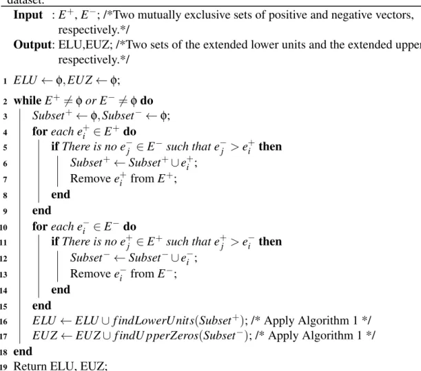
Algorithm 2: General approach to find extended border points in a non-purely monotonic dataset.
Input :E+,E−; /*Two mutually exclusive sets of positive and negative vectors, respectively.*/
Output: ELU,EUZ; /*Two sets of the extended lower units and the extended upper zeros, respectively.*/
1 ELU ←φ,EU Z←φ;
2 whileE+6=φor E−6=φdo
3 Subset+←φ,Subset−←φ;
4 foreach e+i ∈E+do
5 ifThere is no e−j ∈E− such that e−j >e+i then 6 Subset+←Subset+∪e+i ;
7 Removee+i fromE+; 8 end
9 end
10 foreach e−i ∈E−do
11 ifThere is no e+j ∈E+ such that e+j >e−i then 12 Subset−←Subset−∪e−i ;
13 Removee−i fromE−; 14 end
15 end
16 ELU ←ELU∪f indLowerU nits(Subset+); /* Apply Algorithm 1 */ 17 EU Z←EU Z∪f indU pperZeros(Subset−); /* Apply Algorithm 1 */ 18 end
19 Return ELU, EUZ;
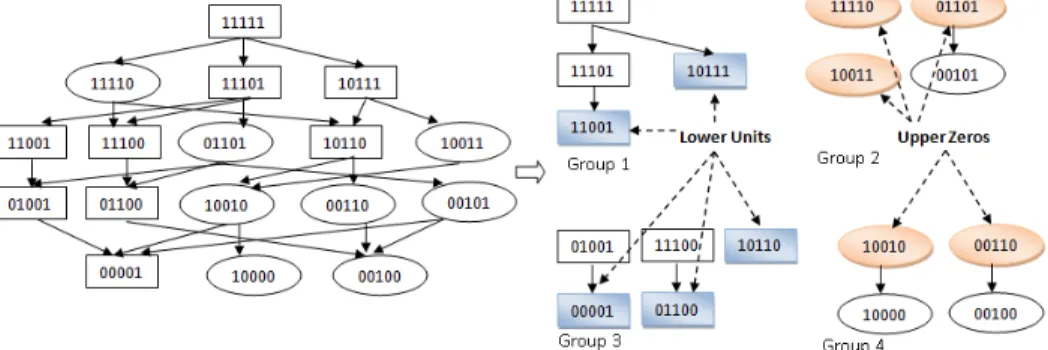
As illustrative examples of the concepts of extended lower units, extended upper zeros, and extended border points, one can consider the dataset in{0,1}5depicted in Table 2.2. The extended lower units ofDare the vectors:{(11001), (10111), (00001), (01100), (10110)}, while the extended upper zeros of D are the vectors:{(11110), (01101), (10011), (10010), (00110)}. The set of its border points is the union of the previous two sets.
TABLE 2.2: An example of a non-purely monotonic datasetDin{0,1}5. Positive vectors (11111), (11101), (10111), (11001), (11100),
(10110), (01001), (01100), (00001)
Negative vectors (11110), (01101), (10011), (00110), (00101), (10010), (10000), (00100)
FIGURE 2.1: The poset for the dataset in Table 2.1 and its border points.
FIGURE 2.2: The poset for the dataset in Table 2.2 and its border points.
2.3
Graphical Representation in Two Dimensions
The previous concepts of the various types of border vectors become easier to comprehend if one considers them in the context of a 2-dimensional partially ordered set or poset (see, for instance, [41, 43]). Such a poset is defined as follows:
Definition 2.15: Given a dataset D, itstwo dimensional poset representationis a graph whose nodes correspond one-to-one to vectors of D. Furthermore, there is an arrow from a node U to a node V , iff U>V .
When a poset representation is used, the data depicted in Table 2.1 correspond to Figure 2.1, while the data in Table 2.2 correspond to Figure 2.2. For the sake of simplicity of the presentation, arrows are shown only for adjacent nodes. One may observe that these graphs can be organized in terms of layers as shown in these figures. The corresponding border vectors (upper zeros and lower units) are also shown in these two figures.
2.4
Data with both Positive and Negative Attributes
In the previous considerations it was assumed that all the binary attributes arepositive. That is, if an attribute has the value 1, then somehow this contributes to the chances for a given vector to be of the positive class value. For instance, in the earlier PC related example, if a particular software item is loaded (i.e., the attribute that corresponds to the loaded/not-loaded state for that software item has value 1), then this contributes to the chances for a vector to be of the positive class value (i.e., the “PC crashes” class value).
Although this may not be as critical for the binary case (as a given binary attribute may be assigned value 1 or 0 depending on how one defines them), it becomes critical when one considers the case when attributes have continuous values. For instance, in a setting with continuous attribute values one may wish to study, say, the performance of a car engine. Then, one may have two mutually exclusive and exhaustive states as follows: The engine needs immediate maintenance (this is the “positive” class or class value 1) or the engine does not need immediate maintenance (this is the “negative” class or class value 0).
In this hypothetical example an attribute that expresses the noise level of the engine could be apositive attribute. This is true because the higher the noise level is, the more likely is that the engine needs immediate maintenance (i.e., it is of the positive class). On the other hand, the number of miles per gallon of fuel could be anegative attributeas the higher the value of that attribute is, the less likely is that the engine to need immediate maintenance.
It is important to state here that in some real-life applications, attributes may not be purely positive or negative. That is, as the value of such attributes increases, it is possible to have certain levels beyond which the chances to be in one class value versus another, may alternate.
For instance, consider a healthy life-style study where among other attributes one of the at-tributes is the amount of daily exercise a person may pursue. For simplicity, assume that the class values are “healthy life-style” (the positive class) and “not healthy life-style” (the negative class). As the amount of exercise increases, say, from 20 minutes per day to 40 minutes, then to 60
min-utes and so on, the chances that we will be in the positive class increase accordingly. However, there is some value for this particular attribute where more increase to its value may not lead to higher chances to be in the positive class. For instance, if one exercises at abusive levels, say 12 or even 14 hours a day, then that may cause some health related problems. For the previous reasons, in this study positive and negative attributes are defined in a non-rigorous manner as follows:
Definition 2.16: An attribute with binary values is called a positive attribute if when it has value 1, then it is more likely for vectors to be in the positive class. Otherwise, it is called a
negative attribute.
Definition 2.17:An attribute withordinal valuesis called apositive attribute, if when the values increase, then it is more likely for vectors to be in the positive class. Otherwise, it is called a
negative attribute.
The following sections will distinguish between positive and negative attributes only. Cases like the one described above, may lead to situations where datasets are not purely monotonic. As it was explained earlier, for non-purely monotonic binary datasets one can decompose them into regions where monotonicity holds locally. Obviously, a dataset with lots of such regions is less overall non-purely monotonic than a dataset with just a few such regions. How this factor and other ones related to monotonicity may impact the learnability of datasets is studied in the following sections.
2.4.1
Identifying the Positive and Negative Attributes
From the previous discussion it follows that there are alternative ways to define what is positive and negative attributes. Thus, there are alternative ways to quantify the way how to determine such attributes. In this study the following approach is used.
Each pair of positive-negative vectors is considered. For each attribute i, let Np,i indicate the number of times attributeiin the positive vectors is greater than the same attributeiin the negative vectors when all pairs are considered. Similarly, letNq,iindicate the number of times attributeiin the negative vectors is greater than the same attributeiin the positive vectors. Then, ifNp,i>Nq,i, the attribute i is assumed to be a positive attribute. If Np,i<Nq,i, it is assumed to be a negative
attribute. Finally, if Np,i=Nq,i, then attribute i is designated as either positive or negative with probability 50%. One may observe here that as more training data are added to a given dataset, the groups of positive and negative attributes may change.
2.4.2
Comparing Vectors with Both Positive and Negative Attributes
Once the positive and the negative attributes have been determined, twon-dimensional vectorsV andW (with binary and/or ordinal attributes) can be defined as follows:V = ((vp1,vp2,vp3, . . . ,vpx), (vn1,vn2,vn3, . . . ,vny)), andW =((wp1,wp2,wp3,. . .,wpx), (wn1,wn2,wn3,. . .,wny)), wheren=x+y. The elementsvpi andwpiindicate the positive attributes of the vectorsV andW, respectively, while vq j and wq j indicate the negative attributes of them. In light of this enhancement, the previous definitions of vectors defined on only positive attributes can be expanded accordingly.
In the new setting a vectorV is said to begreater than or equal to (i.e., it precedes)vectorW (denoted asV W) iffvpi ≥wpi, fori=1,2,3, . . . ,x, and vni≤wni, for i=1,2,3, . . . ,y. In this case one may also say that vectorW isless than or equal to (i.e., it follows) vectorV (denoted asW V). As before, when any of these two ordering relationships can be defined between two vectors, we say that such vectors are related. Otherwise, they are called unrelated. Please note that now the symbolsandare used instead of the previous≥and≤symbols, respectively.
For any pair of vectorsV and W defined as above, if either their positive groups or negative groups are unrelated, then the vectorsV andW are unrelated too. Furthermore, the vectorsV and W are unrelated when they have different number of attributes in either their positive or negative group. It should also be noted here that if both the positive and negative groups of vectorV are at the same time greater than or smaller than those of vectorW, then the vectorsV andW are still unrelated.
For some illustrative examples of the above, consider the four binary vectors defined as follows: V = ((010), (111)),W = ((110), (011)),P= ((100), (010)) andQ= ((011), (110)). Then according to the previous definitions, it follows thatW V and QV. All other pairs are comprised of unrelated vectors.
---Layer 0 ---Layer 1 ---Layer 2 ---Layer 3 ---Layer 4 (11), (00) (10), (00) (01), (00) (00), (00) (01), (10) (01), (11) (11), (01) (10), (01) (01), (01) (00), (10) (10), (11) (11), (11) (10), (10) (11), (10) (00), (11) (00), (01)
FIGURE 2.3: The complete poset whenn=4,x=2, andy=2.
2.5
Graphical Representation for Datasets With Positive and
Negative Attributes
As was the case with binary data that have only positive attributes, the enhanced type of binary data which are defined on both positive and negative binary attributes can be represented graph-ically in terms of posets as well. Figure 2.3 depicts the poset for the complete 4-attribute binary dataset which has two positive attributes and two negative attributes. It is an illustrative example of constructing a poset for such kind of 4-attribute binary dataset. Any 4-attribute binary dataset with two positive and two negative attributes can be defined in this format, but with less than 16 mem-bers is a subset of the one displayed in Figure 2.3. Then, such a binary dataset can be graphically represented accordingly, and this idea can be expanded to display any dataset (i.e., not only binary) with ordinal attributes in two dimensions, provided that the number of vectors is manageable.
The earlier definitions of lower units, upper zeros, border points of purely monotonic datasets still hold as long one defines the ordering relations between pairs of vectors in terms of the two groups of positive and negative attributes. Table 2.3 presents a simple 5-dimensional dataset with purely monotonic data which is defined on three positive attributes and two negative attributes. The same data are also depicted in Figure 2.4 in terms of a poset, and along with the corresponding lower unit and upper zero vectors.
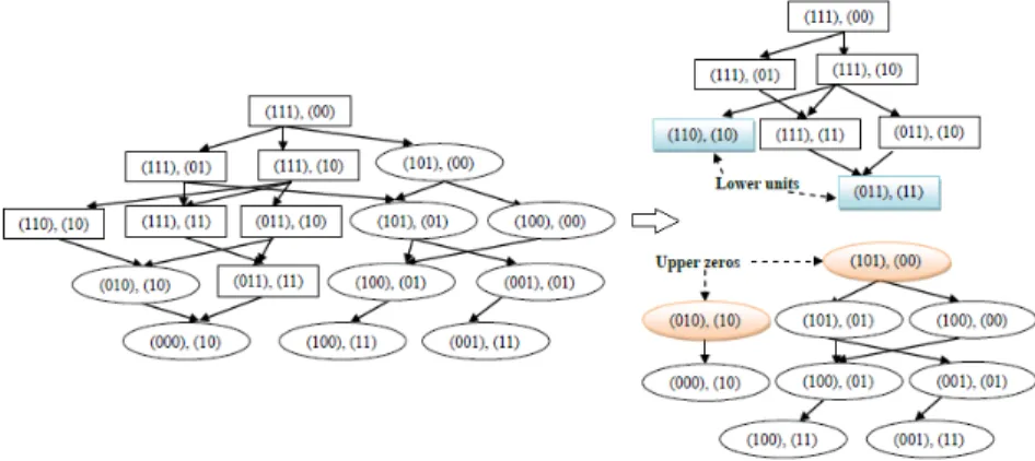
Finally, Table 2.4 presents a dataset which is not purely monotonic and it is defined on three pos-itive attributes and two negative attributes. The corresponding poset representation and a graphical depiction of its lower units and upper zeros are given in Figure 2.5.
TABLE 2.3: An example of a purely monotonic binary training dataset when positive/negative at-tributes are taken into consideration.
Positive vectors ((111),(00)), ((111),(01)), ((111),(10)), ((110),(10)), ((111),(11)) ((011),(10)), ((011),(11))
Negative vectors ((101),(00)), ((101),(01)), ((100),(00)), ((010),(10)), ((100),(01)) ((001),(01)), ((000),(10)), ((100),(11)), ((001),(11))
FIGURE 2.4: The poset for the dataset listed in Table 2.3 and its border points.
TABLE 2.4: An example of a non-purely monotonic binary training dataset when positive/negative attributes are taken into consideration.
Positive vectors ((111),(00)), ((111),(10)), ((110),(10)), ((101),(00)), ((010),(10)) ((000),(10)), ((111),(11)), ((011),(11)), ((101),(01))
Negative vectors ((111),(01)), ((100),(00)), ((011),(10)), ((001),(10)), ((100),(01)) ((100),(11)), ((001),(01)), ((001),(11))
By following the approach described above, the dataset listed in Table 2.4 can be divided into four sub-groups, as shown in Figure 2.5. Based on these sub-groups, the extended lower units are
{((110),(10)), ((101),(00)), ((000),(10)), ((011),(11)), ((101),(01))}, and the extended upper zeros are{((111),(01)), ((100),(00)), ((011),(10)), ((100),(01)), ((001),(01))}.
2.6
Types of Pairs of Vectors
The previous sections formally introduced some key relationships between any two vectors by mostly ignoring their class values. That is, two vectors are either related to each other or are unre-lated. This section discusses how two vectors can be related by also considering their class values. Let us assume that each vector in a dataset is classified to be either positive or negative. By considering such class values, there are five possible relationships between the two vectors in any pair of such vectors. These relationships are: a positive vectorV precedes another positive vector W; a positive vectorV precedes a negative vectorW; a negative vectorV precedes a positive vector W; a negative vectorV precedes a negative vectorW; or the vectorsV andW are unrelated.
For any pair of vectorsV andW, if the vectors are related and they have the same class value, they are said to comprise a pair which is in agreement with the monotonic property, or anAMP pair. In the situation when a negative vectorV precedes a positive vectorW (i.e.,V W), the pair comprised in this order is in conflict with the monotonic property (or it is aCMP pair).
For a pair of vectorsV andW where a positive vectorV precedes a negative vectorW, their class values do no conflict with the monotonic property. This indicates that if one hasVW and knows that vectorV has been classified as positive, then the vectorW can be either positive or negative without conflicting with the monotonic property. A similar observation follows ifV W and the vectorW has been classified as negative. Then the vectorV can be either positive or negative.
Given the above discussion, from now on two monotonically related vectorsVandWof the same class value will be said to comprise a pair which is in agreement with the monotonic property of type 1, or anAMP1 pair. For another pair of vectorsV andW, whereV W and the class value ofV is positive while the class value of W is negative, it is called a pair in agreement with the
monotonic property of type 2, or anAMP2 pair. If the vectorsV andWare unrelated, then the class value of one vector has no effect on that of the other. In this case, they comprise a monotonically neutral pair (or anMNP pair). As it is shown in the experimental section, these types of pairs of vectors play a crucial role in determining how easily a dataset can be accurately analyzed by a large spectrum of classifiers.
More formally, suppose that given are two distinct vectorsV andW defined on n attributes (binary or ordinal in general) and have the same positive and negative attributes. It is also assumed that there are only two classes; the positive and the negative. Next, all the possibilities of the relative relations between any two vectorsV andW and their class values are formally introduced as follows:
Definition 2.18: Two numeric vectors V and W , where V W , constitute a pair which is in agreement with the monotonic property of type 1, denoted as anAMP1 pair, iff they have the same class value.
Definition 2.19: Two numeric vectors V and W , where V W , constitute a pair which is in agreement with the monotonic property of type 2, denoted as anAMP2 pair, iff the class of vector V is positive while the class of vector W is negative.
Definition 2.20: Two numeric vectors V and W , where V W , constitute a pair which is in conflict with the monotonic property, denoted as a CMP pair, iff the class value of V is negative, while the class value of vector W is positive.
Definition 2.21: Two numeric vectors V and W form a monotonically neutral pair, denoted as anMNP pair, iff they are unrelated.
Figure 2.6 depicts a collection of positive and a collection of negative training examples whenn = 4, x = 2, and y = 2. This training dataset is comprised of four positive vectors (denoted with squared shapes) and three negative ones (denoted with oval shapes), and it is a subset of the dataset decipted in Figure 2.3. Then, according to the definitions given above, some examples of AMP1 (ordered) pairs are as follows:{((11),(00)), ((11),(01))}, {((11),(00)), ((11),(10))} and
((01), (00)) ((00), (00)) ((01), (01)) ((01), (10)) ((11), (11)) ((00), (10)) ((11), (01)) ((01), (11)) ((00), (11)) (11), (00) (11), (01) (10), (10) (11), (10) (10), (01) (00), (01) (10), (00)
FIGURE 2.6: Some examples of different types of monotonically related pairs.
{((10),(00)), ((10,(01))}. Some examples of AMP2 (ordered) pairs are{((11),(01)), ((10),(01))}
and{((11),(00)), ((10),(00))}. The only example of a CMP (ordered) pair is{((10),(00)), ((10),(10))}. Some examples of MNP pairs are{((11),(10)), ((10),(01))}and{((10),(00)), ((11),(01))}.
Chapter 3
The Experimental Design for Binary Datasets
This section explores the roles of some potentially important characteristics of numeric datasets, which could be used to predict how difficult it is to analyze a given dataset accurately. As it was stated earlier, the main research hypothesis is that such difficulty is primarily related to the mono-tonic characteristics of a dataset, even if monomono-tonicity occurs partially (i.e., when there are CMP pairs in the datasets).3.1
Design Issues of Experiments with Some Artificial Binary
Datasets
The binary datasets used in this set of experiments were created in different sizes with the value of n(dimensions) ranging from 6 to 60. In each individual experiment, the training data and the testing data are binary datasets with the same number of dimensions (attributes).
As it was stated earlier, this study defines the “difficulty” or learnability of a dataset as how dif-ficult it is to be accurately classified. This is indicated by the average accuracy when it is analyzed by multiple classifiers. The lower the value, the more difficult it is. Moreover, it is assumed that the false positive and the false negative errors are of the same penalty cost. The purpose of the experiments is to generate accurate regression models, which use the monotonic characteristics of the training datasets as the independent variables to formulate their difficulties.
In order to do that, a group of artificial binary datasets were studied in this family of experiments. This group was comprised of “easy” datasets, “difficult” datasets, and datasets with intermediate degrees of difficulty. Four kinds of binary datasets were therefore generated with different mono-tonic characteristics as follows:
1. Random datasets. Such datasets contain vectors with randomly assigned class values. In general, they are expected to have intermediate degrees of difficulty.
2. Datasets without CMP pairs. They are expected to be easy to classify accurately.
3. Datasets which have lots of CMP pairs. This is the opposite case to the one described above. Such datasets are expected to be difficult to classify accurately.
4. Pairs of datasets which have exactly the same border points but have very different numbers of AMP1 pairs. It is expected that the ones with more AMP1 pairs are easier to classify accurately.
3.2
Generating the Binary Experimental Datasets
3.2.1
Generating Random Datasets
The random datasets were generated in a straightforward way. Given are the number of attributes n and the number of selections K. Next, K vectors were selected with replacement with equal probability (i.e., equal to 1/2n). Any duplicate vectors were deleted to make sure that each vector appears only once in the generated dataset. The number of distinct vectors among the K ones is denoted asN(i.e.,K≥N). After that, every vector was assigned to class values 1 or 0 (for positive or negative, respectively) with probability equal to 0.50. The positive/negative attributes of these datasets are unknown, but they can be later determined by the way described in Section 2.4.1. It should be stated here that in this way datasets may not be generated completely randomly as some bias may be present [42].
3.2.2
Generating Datasets Which do not Contain Any CMP Pairs
In order to generate such datasets, one should first decide on the numbers of positive attributes (x) and negative attributes (y), such that x+y=n andx,y≥0. The vectors in these datasets have n attributes while the firstxattributes are considered as positive, and the nextyattributes as negative. After that, a complete (i.e, one of size 2n) n-attribute binary dataset is represented as a 2-D poset, and it is divided into three groups: the positive group, the negative group and the unlabeled group. This is done by determining the values ofK1,K2andK3, such thatK1+K2+K3=n+1 and K1,K2,K3≥0. The topK1 layers comprise the positive group; the vectors located in these layers
are labeled as positive. The bottomK3 layers comprise the negative group; all the vectors located in these layers are labeled as negative. The vectors located in the middle layers are unlabeled.
The following describes how to generate ann-attribute binary dataset withN vectors for given K1,K2,K3,x, and y values. It makes sense that by increasing the value of K1 and decreasing the value ofK3, there should be more positive vectors in the generated dataset, and vice versa.
1. Create a completen-attribute binary datasetD. This dataset should contain 2ndifferent binary vectors.
2. Randomly select a vectorV fromDwithout replacement. Determine the layeriin which it is located by usingi=x−P1+y−P2, whereP1 is the number of the positive attributes in V that are set to value “1” andP2is the number of the negative attributes inV that are set to value “0”, then do the following:
(a) Ifi≤K1, it is a positive vector. (b) Ifi>K1+K2, it is a negative vector.
(c) IfK1<i≤K1+K2, then it can be randomly assigned to either the positive or the neg-ative class with probability equal to 0.50. However, one needs to check if this vector violates monotonicity. For example, if at first a vector is randomly assigned to the neg-ative class, and it precedes some positive vectors generated during previous iterations, then it should be changed to positive to maintain monotonicity.
3. Repeat Step 2)Ntimes to generateN distinct vectors.
3.2.3
Generating Datasets Which Contain Many CMP Pairs
This case is the opposite of the previous one. The challenge is, given the same parameters n,x,y, andN as defined in the previous section, how to assign the class values to theseN binary vectors such that the generated dataset has the maximum (or at least a very high) number of CMP pairs?
Please recall that two monotonically related positive-negative vectors comprise either an AMP2 pair or a CMP pair. However, according to the way one constructs the 2-D poset, the number of
AMP2 pairs should be always larger than that of the CMP pairs. Therefore, the number of CMP pairs should be just less than the number of AMP pairs.
One solution to achieve this goal is to first consider the complete n-attribute binary dataset in its 2-D poset, and label the vectors according to the layers they belong to. More specifically, the vectors in the same layer have the same class value, and their class values are different than those of vectors located at adjacent layers. That is, the top layer, which is comprised of the single vector that has all positive attributes set to “1” and all negative attributes set to “0”, is assigned to the positive class. The second layer is assigned to negative, the third layer to positive, the fourth layer to negative, and so on.
Some experiments were performed to evaluate this method, and Table 3.1 shows some of the experimental results. One can observe from this table that by applying this method, ann-attribute complete binary dataset can have a very similar number of AMP2 and CMP pairs.
Therefore, by using given values for n, x and y, the aim is to have a random dataset with N vectors (whereN ≤2n) such that it has a very large (but not necessarily the maximum) number of CMP pairs. A way to achieve this goal is to first consider the complete case (that is, the case with all 2n vectors). Next, each vector is assigned to a class value in the way mentioned above. Finally, randomly selectN distinct vectors from this complete set. This is how the third group of datasets were generated for this computational study.
It should be stated here that depending on different selections of vectors, an attribute may be recognized as a positive one in some derived datasets, but be considered as a negative one in some other derived datasets, according to the way described in Section 2.4.1.
3.2.4
Generating Datasets Which Have the Same Border Points but Very
Different Monotonic Characteristics
The fourth group of datasets studies the roles CMP and AMP1 pairs play in the learnability of datasets. This group of datasets considered triplets of datasets as follows. First, a dataset was generated randomly as described in Section 3.2.1. Such a dataset may or may not have CMP pairs.
TABLE 3.1: The number of AMP2 and CMP pairs in the completen-attribute binary datasets that are generated by the approach dessribed in Section 3.2.3.
Number of Attributes Number of AMP2 pairs Number of CMP pairs Ratio
n= 5 61 60 1.017 n= 6 182 182 = 1 n=10 14,762 14,762 = 1 n=15 3,587,227 3,587,226 ≈1 n=20 871,696,100 871,696,100 = 1 n=25 2.118×10¹¹ 2.118×1011 =1 n=30 5.147×10¹³ 5.147×1013 =1 n=40 3.039×10¹⁸ 3.039×1018 =1 n=50 1.794×10²³ 1.794×1023 =1 n=60 1.060×1028 1.060×1028 =1
Based on this dataset, two extreme cases are introduced. The first extreme case is to build a dataset which has the same (extended) border points, the same number of positive and negative vectors but has the highest possible number of AMP1 pairs. This is denoted asType I extreme case. The second extreme case is similar to the first one but the interest now is to build a dataset with the smallest possible number of AMP1 pairs. This is denoted asType II extreme case.
Suppose a given dataset is defined onnbinary attributes withxpositive attributes andynegative attributes, it hasN1 positive vectors,N2 negative vectors, and the sizes of the LU and UZ sets are equal toS1andS2, respectively. First, let us assume that it contains no CMP pairs, and its border points (i.e., all the LU and UZ vectors) can therefore be determined by using Algorithm 1. Based on this information, two datasets are generated in order to represent the previous two extreme cases as far as the number of AMP1 pairs is concerned.
To begin with, one needs to first remove all the vectors from the dataset except the border points, and the same number of vectors will be regenerated to becovered by these border points. For the case of the LUs, a vector is said to be “covered” by a lower unit if and only if it precedes this lower unit. For the case of the UZs, a vector is said to be “covered” by an upper zero if and only if it follows this upper zero. For instance, if the vector ((010), (11)) is an LU, then it covers the vector ((110), (11)).
Algorithm 3:Generate an extreme case for a purely monotonic datasetD.
Input : A purely monotonic datasetD.
Output:D Extreme. /* The extreme case ofD*/
1 Pos←φ,Neg←φ,D Extreme←φ,LU←Lower units ofD,UZ←Upper zeros ofD;
2 N1←Number of positive vectors inD,N2←Number of negative vectors inD; 3 S1←Number of vectors inLU,S2←Number of vectors inUZ;
4 n←Number of attributes inD;En←Completen-attribute binary dataset; 5 forEvery vector V ∈Enexcept the LU and UZdo
6 ifV is covered by some members in LUthen 7 Pos←Pos∪V;
8 end
9 ifV is covered by some members in UZthen 10 Neg←Neg∪V;
11 end 12 end
13 Sort the vectors inPosindescending orderby the number ofLUmembers each vector is
covered;
14 D Extreme←D Extreme∪ {The firstN1−S1vectors inPos} ∪LU;
15 Sort the vectors inNegindescending orderby the number ofUZ members each vector is
covered;
16 D Extreme←D Extreme∪ {The firstN2−S2vectors inNeg} ∪UZ; 17 ReturnD Extreme; /* This is for Type I extreme case. */
Every vector except the border points inEn(i.e., the binary space of dimensionn) is examined to see by how many LUs it is covered. Next,these vectors are ranked indescendingorder. Finally, the topN1−S1vectors together with the LUs, are introduced as the new positive vectors.
The negative examples are obtained in an analogous manner. All the vectors except the border points in En are ranked in descending order by how many UZs they are covered by. The top N2−S2vectors and all the UZs are introduced as the new negative examples. This is how the Type I extreme case is generated from a random dataset which has no CMP pairs. This new dataset has many AMP1 pairs because of the way the new positive and negative points are determined.
The Type II extreme case of a given dataset with no CMP pairs can be derived in a similar manner as the previous one. However, in this case the vectors are organized inascendingorder by how many border points they are covered by. Now this dataset has positive and negative vectors which are covered by the least number of border points in the LU and UZ sets. This is how two new
Algorithm 4:Generate an extreme case for a datasetDwhich has some CMP pairs.
Input : A datasetD.
Output:D Extreme. /* The extreme case ofD, which now has some CMP pairs */
1 CMP Vectors←φ,Monotonic Vectors←φ;
2 forEvery vector Vi∈Ddo
3 ifViis found in CMP pairsthen
4 CMP Vectors←CMP Vectors∪Vi; 5 end
6 end
7 Monotonic Vectors←D−CMP Vectors;
8 UseAlgorithm 3(choose different sorting orders to get different extreme types) to derive a
datasetD1fromMonotonic Vectors;
9 D Extreme←CMP Vectors∪D1; 10 ReturnD Extreme;
datasets are derived from a single random dataset without CMP pairs. The previous two approaches are summarized as Algorithms 3. In this algorithm, if one sorts out the vectors in descending order (as is currently shown in Algorithms 3), then the Type I extreme case dataset will be derived as datasetDextreme. If however, the vectors are sorted out instead in ascending order, then the dataset Dextremewill represent the Type II extreme case of the the original datasetD.
Next, let us assume that a given dataset Dcontains some CMP pairs. By removing all its vec-tors that are observed in the CMP pairs, it becomes a dataset with less number of observations and which has no CMP pairs. This is exactly the same type of dataset discussed in the previous case. Thus, from this reduced dataset one can derive two new datasets by implementing Algo-rithm 3 (with different sorting orders). The new generated datasets, together with the vectors that were removed earlier, form the two extreme cases of the datasetD. This approach is described as Algorithm 4.
3.3
Classifiers from WEKA
The classifiers used in these experiments are: a decision tree (J48) [6], a Bayes network [12], a naive Bayes [29], a logistic regression [18], an RBF network [25], a Kstar [27], an LWL [10], an LBK [10], an AdaBoost [21], a Multi-Boost [8], a VFI (Voting Feature Intervals) [15], an
ADTree (Alternating Decision Trees) [20], a BFTree (Best First Tree) [34], a random Forest [4], and SMO [39].
In the experiments, WEKA [46] was implemented as the classification tool. It was used to imple-ment the previous set of classifiers, the parameters of these classifiers are kept at default values as set by WEKA. The experiments used a 10-fold cross validation approach in order to decrease vari-ance. Moreover, each dataset was analyzed by all the classifiers, and the accuracies of the inferred models were recorded. The average accuracy of these models was used as a measure to express their difficulty in learning (i.e., their learnability value).
Chapter 4
The Experimental Study
4.1
Parameters Used to Describe the Monotone Structure of a
Dataset
In order to further explore the relationships between the monotonic characteristics of the datasets and their difficulties, linear regression models were generated using these characteristics as the independent variables, and the difficulties of the datasets as the dependent value.
As discussed above, the difficulty of a dataset can be derived as the average accuracy when it is classified by the classifiers listed in Section 3.3. Moreover, the monotonic characteristics described in Table 4.1 were considered to be strong indicators of the datasets difficulty. In this study, the monotonic characteristicsP1 toP6 were used as the independent (explanatory) variables to build the models. The reason whyP7is excluded is becauseP7=1−P2−P5.
The effectiveness of the chosen monotonic characteristics is in part indicated in Figure 4.1. This figure shows some experimental results performed on binary datasets which have 8 attributes, and each of them contains between 120 and 190 vectors. As can be observed in this figure, it seems that with an increasing number of CMP pairs, the difficulty of accurately analyzing datasets also increases. It also shows that when more unique vectors are observed in CMP pairs, the average accuracy of the derived classification models is going down. Furthermore, given two datasets, the one with more extended border points seems to be more difficult to accurately classify.
At this point one may question what happens if a function is used to transform the data in a different form and possibly dimensionality. This happens, for instance, when kernel functions are used in classification [2, 33]. If the data transformations used can change the ordering (e.g., greater than or equal than) between pairs of vectors, then the values of the six key parameters denoted asP1,P2, . . . ,P6 may change as well. Depending on the way these six parameters change,
TABLE 4.1: The seven monotonic characteristics of the numeric datasets.
P1 = Number of unique vectors found in CMP pairsNumber of all vectors in the training dataset The ratio of the unique vectors that appear in the CMP pairs. P2 = Number of all possible pairsNumber of CMP pairs The ratio of all possible pairs
that are CMP pairs.
P3 = Number of all possible positive-negative pairsNumber of CMP pairs The ratio of the positive-negative pairs that are CMP pairs.
P4 = Number of vectors in the training datasetNumber of extended border points The ratio of the vectors that are extended border points.
P5 = Number of all possible pairsNumber of all AMP1 pairs The ratio of all possible pairs that are AMP1 pairs.
P6 = Number of monotonically related pairs of vectorsNumber of all possible pairs The ratio of the pairs that are monotonically related.
P7 = Number of all possible pairsNumber of all AMP2 pairs The ratio of all possible pairs that are AMP2 pairs.
FIGURE 4.1: Relationships between average accuracy and some monotonic features for binary datasets whenn= 8. They may have different positive/negative attributes.
the transformed dataset may become easier or more difficult to be analyzed. However, if the data transformation cannot affect the ordering of pairs of vectors (and assuming the class values are not affected either), then the learnabilities of the original and transformed datasets will remain identical.
The experiments were performed as follows. First a list of n-attribute numeric datasets were collected as the experimental datasets. Their vectors had been classified as either “postive” or
“negative.” Furthermore, they should present various levels of difficulties, that is, some of the datasets can be classified with high accuracies, while some others should be classified with low accuracies.
Next, the collected experimental datasets were split into two groups as the training and the testing data. Each dataset in the training group was analyzed in two aspects. First it was analyzed by the classifiers mentioned in Section 3.3. The average of the classification accuracies was recorded as its level of difficulty in learning (i.e., its learnability value). Next, its monotonic characteristics were calculated by using the formulas listed in Table 4.1.
After that, a group of linear regression models were generated using the PROC REG function in SAS [37]. The quality of the models was evaluated by their R-Square values and their performance. The models with higher R-Square values are usually more accurate in predicting the difficulty of the testing datasets. The performance of the models can be assessed as follows. First the monotonic characteristics of the testing datasets and their difficulties were calculated in the same way as that of the training datasets. Next, such monotonic characteristics were used in the generated regression models to predict the difficulties of the corresponding testing datasets. The difference between the predicted difficulties and the real difficulties are what is of interest. If the deviations were small, a regression model was believed to be an accurate one. Therefore, the mean of the deviations is an important evaluator as well.
Furthermore, the variance of the deviations is another issue. Two regression modelsAandBmay have similar means of deviations. However, the deviations produced by modelAmay have a large variance while the ones produced by modelBare more stable. That is, model Amay make some predictions very accurately but be very inacurate in some other predictions. Meanwhile, modelB does all the predictions with similar deviations. In such cases one would prefer modelB since it has less risk of generating meaningless predictions (i.e., predictions that are very different from the actual values). Therefore, in this study, the deviations were analyzed by their mean and their 95% confidence intervals.
The next two sections provide the details of the experiments performed on some binary and continuous numeric datasets, respectively. The experimental results would be provided together with the analysis.
4.2
Experiments with Binary Datasets
4.2.1
Experiments on Artificial Binary Datasets
The monotonic characteristics of the datasets are the monotonic relationships between its pairs of vectors. If a dataset has too few pairs of vectors that are monotonically related, then the values of its monotonic characteristicsP1toP6will all be close to 0, and therefore no useful information can be provided when generating regression models.
Therefore, the immediate problem is, what is the precondition under which the proposed ap-proach can generate accurate regression models? A set of experiments were designed to explore this issue. The experimental datasets used in this set of experiments are some artificial binary datasets with dimensionsn = 10, 14, 18 and 22. Each dataset had from 400 to 1,500 vectors and each vector was labeled as either “positive” or “negative.”
At the beginning, the experimental datasets were categorized by their dimensions, four groups of datasets were therefore generated. Furthermore, the datasets in each group were further split into several experimental groups by their monotonic characteristic P6 (the ratios of the pairs that are monotonically related), and each experimental group had around 300 datasets. A list of regression models were generated from these experimental groups, and their R-Square values are what is of interest. Figure 4.2 shows some of the experimental results.
As one can observe from this figure, the R-Square values of the models were consistently above 0.92 when the experimental datasets have more than 6% pairs of vectors that are monotonically related. In other words, it seems that under this simple condition the quality of the models can be somehow ensured. Therefore, this study only focuses on numeric datasets that have more than 6% monotonically related pairs.
FIGURE 4.2: The R-Square values of the models generated from artificial binary datasets with different dimensions.
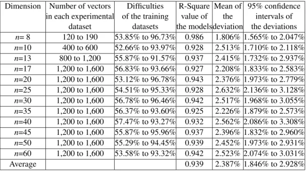
The above four groups of datasets forn=10, 14, 18 and 22 served as pilot tests. Next, artificial datasets were generated according to the procedures described in Section 3.2. Now the dimensions ranged from 8 to 60. In these experiments, the datasets were grouped by their dimensions, and each group contained about 450 datasets, where 350 of them were randomly selected for training and the remaining 100 were used for testing. Furthermore, according to the way they were generated, the difficulty of these datasets would also vary significantly. The quality of the regression models would be evaluated by their R-Square values and also their performance in predicting the difficul-ties of the testing datasets. Tables 4.2 and 4.3 list some experimental results on these datasets.
As one can observe from this table, when there are sufficient number of vectors that are mono-tonically related in a dataset, the difficulty of this dataset can be accurately predicted by analyzing its monotonic characteristics. The R-Square values for all the models listed in this table are greater
TABLE 4.2: The regression models generated for different dimensions of artificial binary datasets. Dimensions Regression models
N= 8 Y = 0.532 + 9.345×P1 - 22.55×P2 - 0.312×P3 - 0.236×P4 + 1.734×P5 + 0.209×P6 N= 10 Y = 0.737 + 10.19×P1 - 44.48×P2 - 0.103×P3 - 0.260×P4 + 1.104×P5 - 0.013×P6 N= 13 Y = 0.891 + 10.43×P1 - 41.27×P2 - 0.387×P3 - 0.330×P4 + 0.307×P5 + 0.151×P6 N= 17 Y = 0.746 + 14.42×P1 - 71.86×P2 - 0.189×P3 - 0.253×P4 + 0.019×P5 + 0.628×P6 N= 20 Y = 0.686 + 26.76×P1 - 87.84×P2 - 0.126×P3 - 0.118×P4 - 1.017×P5 + 0.879×P6 N= 25 Y = 0.857 + 26.78×P1 - 56.75×P2 - 0.092×P3 - 0.384×P4 + 1.147×P5 - 0.201×P6 N= 30 Y = 0.789 + 18.16×P1 - 46.25×P2 - 0.170×P3 - 0.216×P4 + 0.084×P5 + 0.133×P6 N= 35 Y = 0.746 + 11.64×P1 - 71.38×P2 - 0.189×P3 - 0.253×P4 + 0.019×P5 + 0.628×P6 N= 40 Y = 0.686 + 23.86×P1 - 78.85×P2 - 0.126×P3 - 0.118×P4 - 1.017×P5 + 0.879×P6 N= 45 Y = 0.857 + 22.35×P1 - 69.11×P2 - 0.092×P3 - 0.384×P4 + 1.147×P5 - 0.201×P6 N= 50 Y = 0.789 + 18.03×P1 - 76.25×P2 - 0.164×P3 - 0.216×P4 + 0.084×P5 + 0.133×P6 N= 60 Y = 0.789 + 16.63×P1 - 59.64×P2 - 0.170×P3 - 0.143×P4 - 0.043×P5 + 0.167×P6
TABLE 4.3: Details of the regression models listed in Table 4.2.
Dimension Number of vectors Difficulties R-Square Mean of 95% confidence in each experimental of the training value of the intervals of
dataset datasets the modelsdeviation the deviations
n= 8 120 to 190 53.85% to 96.73% 0.986 1.806% 1.565% to 2.047% n=10 400 to 600 52.66% to 93.97% 0.928 2.513% 1.710% to 2.118% n=13 800 to 1,200 55.87% to 91.57% 0.937 2.415% 1.732% to 2.937% n=17 1,200 to 1,600 56.83% to 93.66% 0.927 2.208% 1.833% to 2.583% n=20 1,200 to 1,600 53.12% to 96.78% 0.943 2.376% 1.973% to 2.779% n=25 1,200 to 1,600 54.51% to 95.33% 0.928 2.632% 2.136% to 3.128% n=30 1,200 to 1,600 56.78% to 96.46% 0.942 2.517% 1.968% to 3.055% n=35 1,200 to 1,600 56.37% to 93.60% 0.925 2.226% 1.879% to 2.573% n=40 1,200 to 1,600 57.47% to 93.27% 0.932 2.562% 2.086% to 3.308% n=45 1,200 to 1,600 55.87% to 95.96% 0.937 2.396% 1.832% to