Tensor Network States: Optimizations and Applications in Quantum Many-Body Physics and Machine Learning

(1)

University of Central Florida University of Central Florida

STARS

Electronic Theses and Dissertations, 2020-

2020

Tensor Network States: Optimizations and Applications in

Quantum Many-Body Physics and Machine Learning

Justin Reyes

University of Central Florida

Find similar works at: https://stars.library.ucf.edu/etd2020

University of Central Florida Libraries http://library.ucf.edu

This Doctoral Dissertation (Open Access) is brought to you for free and open access by STARS. It has been accepted for inclusion in Electronic Theses and Dissertations, 2020- by an authorized administrator of STARS. For more information, please contact STARS@ucf.edu.

STARS Citation STARS Citation

Reyes, Justin, "Tensor Network States: Optimizations and Applications in Quantum Many-Body Physics and Machine Learning" (2020). Electronic Theses and Dissertations, 2020-. 275.

(2)

TENSOR NETWORK STATES: OPTIMIZATIONS AND APPLICATIONS IN QUANTUM MANY BODY PHYSICS AND MACHINE LEARNING

by

JUSTIN REYES

B.S. in Physics, University of Central Florida, 2015

A dissertation submitted in partial fulfilment of the requirements for the degree of Doctor of Philosophy

in the Department of Physics in the College of Sciences at the University of Central Florida

Orlando, Florida

Summer Term 2020

(3)

c

(4)

ABSTRACT

Tensor network states are ubiquitous in the investigation of quantum many-body (QMB) physics. Their advantage over other state representations is evident from their reduction in the computa-tional complexity required to obtain various quantities of interest, namely observables. Addition-ally, they provide a natural platform for investigating entanglement properties within a system. In this dissertation, we develop various novel algorithms and optimizations to tensor networks for the investigation of QMB systems, including classical and quantum circuits. Specifically, we study optimizations for the two-dimensional Ising model in a transverse field, we create an algorithm

for the k-SAT problem, and we study the entanglement properties of random unitary circuits. In

addition to these applications, we reinterpret renormalization group principles from QMB physics in the context of machine learning to develop a novel algorithm for the tasks of classification and regression, and then utilize machine learning architectures for the time evolution of operators in QMB systems.

(5)

This dissertation is dedicated to my Lord and Savior Jesus Christ, "in whom are hidden all the treasures of wisdom and knowledge" – Colossians 2:3

(6)

ACKNOWLEDGMENTS

The completion of this dissertation has been made possible by the determination and dedication of a few special people in my life. I am thankful first to my Lord Jesus Christ, who has blessed me with the opportunity to pursue this degree, and also supported me through the process.

Secondly, I am grateful to my wife Danielle Reyes for her consistent motivation and support. I would have given up on this endeavor long ago without her. She is my biggest supporter in all of my academic adventures.

I would like to thank my family for encouraging me and remaining by my side even if my research made little to no sense to any of them.

Finally, I would like to thank my advisor Dr. Eduardo Mucciolo, for all of his hard work in guiding me through the process of becoming a doctor of physics. He has been a consistent example to me of the dedication, endurance, patience, and humility necessary to appropriately perform scientific research. Without him, I would have no idea what I am doing.

A special thank you to Dr. Andrei Ruckenstein, Dr. Claudio Chamon, Dr. Stefanos Kourtis, and Lei Zhang for collaborating with me on many projects, specfically the work detailed in chapters 5, 6, and 7. In each of these cases, the team was instrumental in both proposing novel ideas and in modifying the implementations of code throughout each project. Similarly, thank you to Dr. Dan Marinescu for working patiently with me on my very first project, for which I am sure my inexperience showed greatly. Thank you to Dr. Miles Stoudenmire for your collaboration on the project found in chapter 8, providing me access to your iTensor library and coming up with the ideas behind the network architecture and its applications. This truly allowed me to pursue my interests in machine learning. Also, thank you to Sayandip Dhara for providing the necessary

(7)

input data for the machine learning tasks performed in chapter 9, and also for being an office mate, a friend, and someone to discuss research ideas with.

(8)

LIST OF FIGURES

Figure 1.1: Top: Tensor diagrams for a scalar, a matrix, and an order-3 tensor. Bottom: Tensor network diagrams involving three tensors generated from the decom-position of a scalar (left) and an order-3 tensor (right). . . 5

Figure 1.2: A tensor diagram for a six-site MPS with periodic boundary conditions (top), and a tensor diagram for a six-site MPS with open boundary conditions (bot-tom). . . 7

Figure 1.3: A diagrammatic representation of the successive Schmidt decomposition steps which transform an initial state_|Ψiinto a right canonical MPS. First, an SVD is performed between site one and the rest of the system. Then, the singular values λ are multiplied to the right withV†. These steps are repeated over

every site until the decomposition is complete. . . 9

Figure 1.4: An example tensor diagram for the calculation of the expectation value_hO_i.

The result is computed by contracting all connected bonds. Here, O is a

two-body operator. . . 12

Figure 1.5: A tensor diagram for a two-dimensional, twenty-site, rectangular PEPS with open boundary conditions. Black lines indicate internal bonds (indices), while grey lines indicate physical bonds (indices). . . 13

Figure 2.1: A graphical representation of a TLU (perceptron). . . 17

Figure 2.2: A graphical representation of an MLP consisting of an input layer, and one

(15)

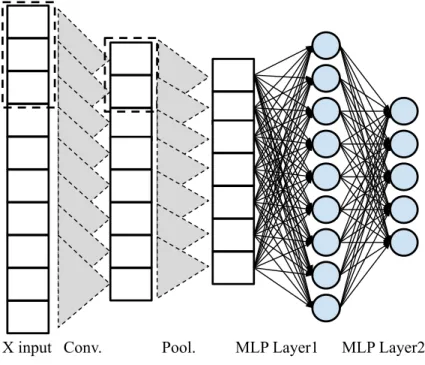
Figure 2.3: A graphical representation of a CNN taking in one-dimensional input, apply-ing a convolution filter of size three, and a poolapply-ing filter of size two. The output of these filters is passed into a two-layer MLP. . . 20

Figure 2.4: A graphical representation of an RBM having four visible units with biases

a_iand six hidden units with biasesb_i. . . 21

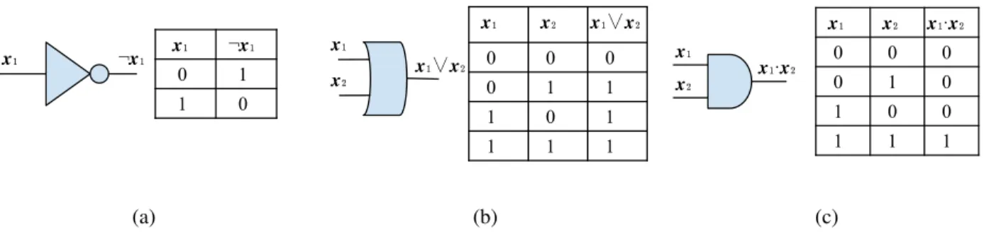
Figure 3.1: Circuit diagrams and truth tables for the NOT gate (a), the OR gate (b), and the AND gate (c). Input to output is read from left to right. . . 23

Figure 3.2: Circuit diagram and truth table for a half-adder circuit acting on two bitsx₁

andx₂. The summation of the two inputs is contained inS, while the carry value is contained inC. . . 25

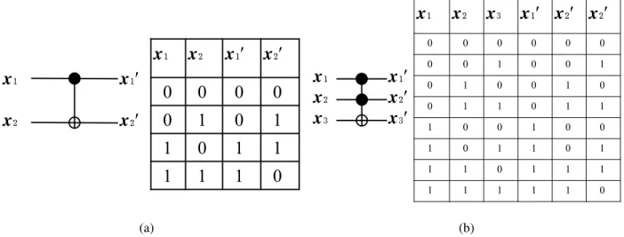
Figure 3.3: Circuit diagrams and truth tables for the CNOT gate (a), and the Toffoli gate (b). Input to output is read from left to right. . . 26

Figure 3.4: A quantum circuit diagram with four qubitsφi initiliazed on the left, trans-formed by a random sequence of gates selected from the universal gate set {CNOT,H,S,T_}, and measured on the right by projectors. . . 29

Figure 4.1: A schematic for the AWS cloud. Depicted is a local computer which con-nects and submits computational scripts to a personally assigned virtual pri-vate cloud (VPC), consisting of inter-connected instances (white blocks) each having their own set of virtual processors (vCPUs) and access to an elastic

(16)

Figure 4.2: Schematics for two square TN contraction orderings and parallel partition-ings. In a) the row contraction and parallel partition are shown, resulting in

a final column of tensors each with bond dimensionDL. In b) the quadrant

contraction and parallel partition are shown, resulting in a ring of tensors with bond dimensionDL/2. . . 34

Figure 4.3: Results for the computational time needed to compute the contraction of TN square lattices sizedL= [5,12]. Different lines correspond to different values

of the fixed maximum bond dimensionχ=√D. Memory limitations prevent

simulation of larger sized systems for larger sized bond dimensions. . . 36

Figure 4.4: Results for the time to complete the contraction of square TN lattices sized

L= [5,10]. Differing lines represent different contraction orderings and schemes: row contraction (black), quadrant contraction (red), and CTF contraction (blue). The quadrant contraction shows a more favorable scaling for larger lattice sizes. . . 37

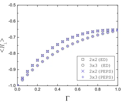
Figure 4.5: Results comparing exact diagonalization calculations to the final energies calculated for the PEPS ITE algorithm applied to the transverse field Ising model. Here lattice sizes areL={2,3_}, spin couplingJ=1, transverse field strengthΓvaries from 0 to 1, and time steps are taken asδ τ =3/100. . . 40

(17)

Figure 4.6: A comparison between the PEPS ITE alogrithm and a TTN algorithm for calculating the ground state expectation values (a)_hσxiand (b)hσzzifor the

two-dimensional Ising model with spin coupling J=1 and transverse field

strengths Γ= [0,4]. Comparisons are made between square lattices sized

L=6. Also depicted are the values obtained for lattice sizeL=4. ITE

cal-culations were done with time stepδ τ =3/75 and maximal bond dimension

χ=4. . . 41

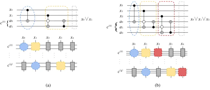
Figure 5.1: A schematic detailing the tensor network embedding of boolean circuits. In (a) a single #2SAT clause is shown above, with gates grouped by dashed lines. The blue group becomes the CIRCLE gate, the yellow group becomes the BLOCK gate, and the grey group is an ID gate used to create uniformity throughout the tensor network. Below, each clause ancillary bus c(i) forms the horizontal bonds of the network, while bitsxiform the vertical bonds. In (b) a single #3SAT clause is shown above, with gates also grouped by dashed lines. The blue group becomes the CIRCLE gate, the group becomes the BLOCK1 gate, the red group becomes the BLOCK2 gate, and again the grey group becomes the ID gate used to create uniformity in the tensor network. Horizontal bonds are given by each ancillary busc(i) and vertical bonds are given by bitsx_i . . . 44

Figure 5.2: A schematic of Boolean circuit gates for (a) the #2SAT and (b) the #3SAT circuits being converted into tensor networks with a uniform distribution of tensors throughout. Horizontal bonds represent bus auxiliary bits and vertical bonds represent bits. . . 46

(18)

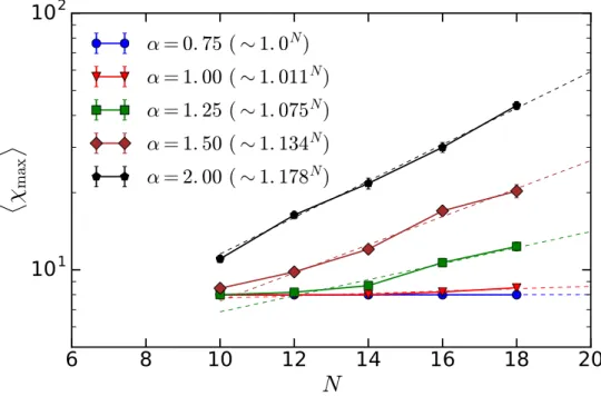
Figure 5.3: Results of the average runtime_hτito solution for the #3-XORSAT problem

with varying number of bitsN = [10,150] and differing clause-to-bit ratios

α. Dashed lines fit exponential scales to the final four points of eachα curve. 49

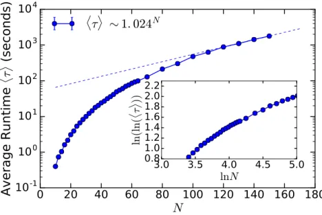
Figure 5.4: Scaling of the average runtime _hτi for clause-to-bit ratio α =0.75. This

regime is below the satisfiability transitionα =0.92. The inset displays a

linear trend in the plot of ln(lnτ)vs lnN, indicating a polynomial scaling of

the runtime. . . 50

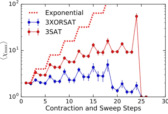
Figure 5.5: Calculations of the average maximum bond dimension_hχmaxioccurring

dur-ing each step of the ICD. When a decimation (contraction) step occurs, the bond dimensions are seen to increase, while during the compression (SVD sweeps) steps, bond dimensions decrease. Measurement were made for an

clause-to-bit ratioα =1 for both the #3-SAT and #3-XORSAT instances. . . 51

Figure 5.6: Calculations of the average maximal bond dimension_hχmaxioccurring

through-out the computation of solutions for the #3-SAT problem. Solutions are gath-ered over varying clause-to-bit ratiosα∈[0.75,2]. Belowα=1, the scaling

of_hχmaxiappears to be sub-exponential. . . 52

Figure 6.1: A schematic for the transformation of a quantum circuit to a π/4 rotated

rectangular tensor network. Beginning with a circuit diagram, with qubits initially in the state _|φii, the transformation U is decomposed into 2-qubit operators which are reshaped into tensors. Dashed lines indicate periodic

(19)

Figure 6.2: A tensor diagram for the decomposition rotation of the initialπ/4 rectangular

lattice. a) An SVD decomposition is performed over a group of 4 neighboring tensors. b) Tensors generated in the bulk of the neighbors are grouped and contracted together. c) Steps (a) and (b) are performed over every group of 4 tensors until the network is rotated. . . 60

Figure 6.3: Entanglement Entropy S for MPS simulations of N =10 qubits evolved to

the quantum chaotic state by application of gates taken from the Clifford + T gate set. In (a), the circuit is constructed using dense gates. In (b), the circuit is constructed using dilute gates. The entropy is averaged over every two-site partitition in the qubit chain and over every realization. For both cases, the chaotic state is achieved when the entanglement has saturated to its maximal value. Only 5 realizations were used for each circuit type. . . 61

Figure 6.4: A comparison of the distribution of amplitudes taken over the projectorP0

for both the dense and dilute tilings of sycamore circuits withN =8 qubits. The distributions are similar and in agreement with the quantum chaotic

Porter-Thomas (PT) distribution. Averages were taken over 5000 realizations. 62

Figure 6.5: A comparison of the average maximum bond dimension,_hχmaxi, encountered

at a given ICD step for dense and dilute tiling of random sycamore circuits

with N =8 qubits. Each ICD step consists of ten decomposition sweeps,

(20)

Figure 6.6: Plot of the average maximum bond dimension_hχmaxioccurring for each ICD

iteration for varying entangling gate concentrations. Random circuits are constructed with 12 qubits and a circuit depth of 24. Gates are selected from the UCliff+T gate set, with the concentration determined by the number of

CNOT gates present in the system. . . 64

Figure 6.7: A tensor diagram for a 4-qubit random quantum circuit with gates taken from

Usyc. Bonds dimensions are color-coded. The horizontal arrow indicates a

single pass of Schmidt decompositions over every tensor pair. The vertical arrow indicates progression to the next decimation step in the ICD algorithm. It is clear that as the bond dimensions continue to grow through the decima-tion process up to the final step. . . 66

Figure 6.8: Distribution of the squared amplitudes for random circuits generated from theU_Cliff₊_T andUsycgate sets. For the former, circuits were simulated with

N=44 qubits, and for the latter, circuits were simulated withN=36 qubits. Distributions are compared to the Porter-Thomas distribution. Statistics were gathered over 1000 instances each. . . 67

Figure 7.1: (a) A gate and and projector are reshaped into tensor Tg, which is then de-composed via SVD, and the tensor projector aggregated together with the gate. (b) The procedure for reshaping a single tensor and projector is applied over a full circuit until a rectangular tensor network is formed. . . 73

(21)

Figure 7.2: Level spacing ratio distributions for the entanglement spectrum in the three phases of entanglement. Distributions are taken from circuits constructed

from the random Haar-measure withNbits and with depthd=N. (a)

Volume-law phase at p=0.2, as indicated by the GUE distribution with level repul-sion in the limitsr_→0 and a Gaussian tail atr_→∞. (b) Residual repulsion

phase at p=0.35. Level repulsion disappears at r_→0 while a majority of

levels show level repulsion as indicated by the presence of a peak at finite

r. (c) Poisson phase at p=0.5. The spectrum displays an absence of level repulsion in similarity to the Poisson distribution. The insets show the distri-butions in log-log scales in order to capture their behavior at the tails. In (a),

results are obtained from 500 realizations forn=20 and from 1000

realiza-tions forn<20. For (b) and (c), , results are obtained from 1000 realizations for up ton=24. . . 75

Figure 7.3: Level spacing ratio distributions for the entanglement spectrum in the three phases of entanglement. Distributions are taken from circuits constructed from the universal gate setUsyc=

√

X,√Y,√W,fSim withNbits and depth

d=2N. (a) Volume-law phase atp=0, again indicated by the GUE statistics in the level spacing. (b) Residual repulsion phase at p=0.2> p_s =0.15, where the shifted peak has morphed into a plateau extending from zero. (c) Poisson phase at p =0.4> p_c =0.35. The insets show the distributions in log-log scales in order to capture their behavior at the tails. Results are obtained from 500 realizations up ton=16. . . 76

(22)

Figure 7.4: Level spacing ratio distributions for block-diagonal GUE matrices composed

of two blocksAandB. The overall size of the composite matrixABis 100_×

100, while the relative sizes of blocksAandBvary. In (a) blockAis 10_×10, while blockBis 90_×90. In (b) blockAis 30_×30, while blockBis 70_×70.

In (c), blockA andBare both 50_×50. Distributions are gathers over 5000

samples for each block diagonal structured GUE matrix. . . 80

Figure 8.1: A tensor diagram depicting two layers of a MERA tensor network, showing

the unitary condition obeyed by the disentanglersU and isometric condition

obeyed by the isometriesV. . . 82

Figure 8.2: The tensor diagram for the model we use for classification and regression, showing the case of three MERA layers. Each input dataxis first mapped into

a MPS_|Φ(x)i, then acted on by MERA layers approximating Daub4 wavelet

transformations. At the top layer, the trainable parameters of the modelW

are decomposed as an MPS. Because all tensor indices are contracted, the output of the model is a scalar. . . 83

Figure 8.3: (a–d) the decomposition of each transformation element D₁₋₄ into the uni-taries and isometries of the wavelet MERA. The complete Daub4 wavelet transformation over data elementsx₁₋₄is given by the contraction over

(23)

Figure 8.4: A tensor digram depicting the local update ofW(MPS) is as follows: a) select a pair of neighboringW(MPS) tensors as B_{j j}₊₁, b) compute the gradient of the cost over all training examples, c) updateB_{j j}₊₁, and d) decompose back into two MPS tensors using a truncated SVD. This is done for each pair in

the MPS, sweeping back and forth until the cost is minimized. . . 91

Figure 8.5: Tensor diagrams detailing the steps of our machine learning wavelet MERA alorithm. In a) the training sets are embedded into an MPS (light blue) and coarse grained through the wavelet MERA for training of the weight MPS (white) at the top most layer. b) Once training is complete, the weight MPS is fine grained through the wavelet MERA by applying isometries and unitaries. c) Training is carried out on the training set at the finer scale . . . 93

Figure 8.6: Results showing the percentage of correctly labeled samples (training set as solid lines and test set as dashed lines) for the audio experiment. The results were collected after trainingWover input data coarse grained throughN_d₄+1 Daub4 wavelet transformations and then again after being projected back and trained atN_d₄layers. Each data set was initially embedded into a vector of 219

elements and coarse grainedN_h₂ Haar wavelet transformations before being

embedded in the Daub4 wavelet MERA. The optimization was carried over 5 sweeps, keeping singular values above∆=1×10−14. . . 95

(24)

Figure 8.7: Results for the average absolute deviation _hεi (lower is better) of the

pre-dicted output and target output for the temperature experiment. Restuls were gathered after trainingW(MPS)over input data coarse grained throughN_d₄+1 wavelet layers and projected back toN_d₄ layers. Each data set was initially constructed by selecting p data points within the setN_{f it}. The optimization

was carried over 40 sweeps, keeping singular values above∆=1×10−9. . . 96

Figure 9.1: A schematic of MLP receiving input vectors having two elementsxi, applying a single layer of four perceptrons with weights a_i, and outputting a single valuey. . . 102

Figure 9.2: A schematic representation of a MLP used for regression. First the data set

X is partitioned into examples for training, with the true label beingybeing the data pointx_p₊₁, where pis the size of a training window. These training

sets are passed to a MLP, where the cost of outputy0 is measured againsty

and optimized the weightsai. . . 105

Figure 9.3: Results for the dynamics of the_hSz_ioperator measured for the ten-site one-dimensional Ising model with spin couplingJ=1 and transverse field strength

Γ=1. MLP calculations are compared with TEBD calculations and exact

diagonalization results. The inset shows the absolute deviations of both the MLP and MPS calculations as compared to the exact results. . . 107

Figure 9.4: Results for the dynamics of the _hSx_i operator measured for the twelve-site

one-dimensional XXZ model with J_⊥ =2, J_z=1, and Γ=1. MLP

calcu-lations are compared with TEBD calcucalcu-lations. The inset shows the absolute deviation of between the MLP and TEBD. . . 109

(25)

LIST OF TABLES

Table 5.1: Truth table and the corresponding tensor components for the CIRCLE gate. On the input side,α =x, β ≡(ab) =21a+20b; on the output side,γ =x0, δ ≡(a0b0) =21a0+20b0. All unspecified components are zero. . . 47

Table 5.2: Truth table and the corresponding tensor components for the BLOCK gate. On the input side,α =x, β ≡(ab) =21a+20b; on the output side,γ =x0, δ ≡(a0b0) =21a0+20b0. All unspecified components are zero. . . 47

(26)

CHAPTER 1: INTRODUCTION TO TENSOR NETWORK STATES

Introduction

The work in this dissertation is interdisciplinary in nature, drawing from the disciplines of physics, mathematics, and computer science. As such, it is necessary to provide a review of a few key concepts from these disciplines which are relevant to the projects contained herein. In chapter 1, we will first introduce tensor networks in the context of quantum many-body physics. In chapter 2, we will review important features of machine learning, particularly focusing on the use of neural networks. We will finish the review material in chapter 3 by highlighting a few key elements in quantum circuit modelling. All of these areas of study will come together in the projects discussed in chapters 4 – 9. Finally, summary conclusions and future work will be presented in chapter 10.

A Limitation in Quantum Many-Body Systems

We begin our review by discussing some fundamental notions from quantum many-body (QMB) physics. The study of QMB physics is primarily concerned with understanding how emergent (macroscopic) properties arise from microscopic descriptions of quantum systems involving many particles [1]. Examples of such investigations within the context of condensed matter physics

in-clude understanding the mechanisms behind high-T_csuperconductivity [2], determining the bounds

on the transition between many-body localized (MBL) and eigenstate thermalization hypothesis (ETH) phases [3], and understanding topologically order phases [4], among others. Often, in order to find solutions to these problems, simplified models are constructed as a representation of the system in question. Though they are not full descriptions of the system, these models are defined in such a way that they implement all the relevant interactions being considered in the problem.

(27)

Some particular models of interest which are ubiquitous in condensed matter physics are the Hub-bard model, the Heisenberg model, and the Anderson model [5].

When specifying a model, it is necessary to define a Hamiltonian operatorH . This operator acts

on a system state vector_|ψiaccording to the Schrodinger wave equation as

H |ψi=id|ψi

dt , (1.1)

withi2=₋1 (we work with units such that the rationalized Planck constant ¯h=1). This Hamil-tonian operator measures the total energy within the system. When it is associated with a basis set {|φii}, the Hamiltonian can be represented by a matrix with elements given by

Hi j=hφi|H |φji. (1.2)

The choice of basis determines the vector space that the Hamiltonian acts on. This vector space over complex numbers is called a Hilbert space [6]. A basis of particular interest is the one in which the basis states satisfy the time independent Schrodinger wave equation

H |φji=Ej|φji. (1.3)

The states contained within this basis are said to be eigenstates of the Hamiltonian, with

(28)

diagonal and the time dependence of each basis state can be given as

|φj(t)i=e−iEjt|φji. (1.4)

It is clear from Eq. 1.4 that the time dependence for eigenstates is trivial, producing changes only in the phase of the state. For this reason, eigenstates are also calledstationary states [6]. If this basis set is known, the full state of the system_|Ψiat a timet can be expanded as

|Ψ(t)i=

∑

j

C_j_|φj(t)i, (1.5)

withC_jbeing a complex-valued probability amplitude such that the probabilityP(φj)of measuring energyE_jfor state_|φjiis

P(φj) =|Cj|2. (1.6)

From this expansion, the expectation value of any relevant quantity given by the action of an operatorO can be calculated directly as

hOi=hΨ(t)|O|Ψ(t)i=

∑

j

|C_j_|2_hφj(t)|O |φj(t)i. (1.7) However, it is often the case (particularly when considering systems involving many particles), that the Hamiltonian cannot be exactly diagonalized, and approximate or numerical methods must be employed [5, 7]. The reason for this is two-fold. Firstly, the Hamiltonian may be composed of

(29)

operators ˆhi, e.g.,H =∑ihˆi, which do not commute, namely,

_ˆ

h_i,hˆ_j=hˆ_ihˆ_j₋hˆ_jhˆ_i₆=0 fori₆= j. (1.8)

The non-commutability of these operators guarantees that a complete set of simultaneous

eigen-states cannot be found [5, 7], making it difficult to determine the eigeneigen-states ofH . The second

reason is that the size of the Hilbert space is known to grow exponentially with the number of particles under consideration [5, 7]. This feature prevents the numerical studies of larger system sizes. While the former limitation is an analytic consequence determined by the definition of a given model, the latter is a computational limitation that can be overcome in part or minimized by reformulating the problem statement in the language of tensor networks.

Tensor Network States

To understand tensor network states and their use in QMB physics, it is first necessary to introduce the mathematical structure of tensors. A tensor is an algebraic structure which serves as high-order generalization of a vector [8]. By this it is meant that a tensor is a collection of scalar quantities (elements) which are tabulated by a set of indices~ν ={ν1,ν2,ν3, ...}. Theorderof a tensor (some

times called rank) is given by the number of indices necessary to specify a unique element within the tensor [8]. Under this definition, a scalar, a vector and a matrix are equivalent to a zeroth-order, first-order, and second-order tensor, respectively. While the indices of a tensor may have specific designations (e.g., space, time, momentum, spin, etc) and be related by specific transformation properties, here we do not make any assumption in both regards. Formally, a tensor of arbitrary order can be constructed by successively taking the Cartesian products of index sets defined over vector spaces. Various operations can be applied to tensors. Take, for example, a third-order tensor

(30)

SCALAR VECTOR MATRIX

TENSOR NETWORKS

Figure 1.1: Top: Tensor diagrams for a scalar, a matrix, and an order-3 tensor. Bottom: Tensor network diagrams involving three tensors generated from the decomposition of a scalar (left) and an order-3 tensor (right).

T_{i jk}. This tensor can me multiplied by a scalar factorα as

T_{i jk}0 =αTi jk, (1.9)

or added with another tensor of equal order,S_{i jk}, as

(T+S)i jk=Ti jk+Si jk, (1.10)

or contracted with another tensor of arbitrary order. This final operation is performed as a summa-tion over all possible values taken by common indices between the two tensors [8]. As a specific

(31)

example, contractingT_{i jk} with a second-order tensor,S_kl, is given as

(T S)i jl=

∑

k

T_{i jk}S_kl. (1.11)

Notice that the result is itself another tensor, composed of indices which were not repeated between tensorsT andS. In light of this, we can say that any tensor can be rewritten (decomposed) as a set of tensors which are to have a specific pattern of contraction (geometry). This set of tensors is called

a tensor network. Before continuing further, it is beneficial to introduce a graphical notation for

tensors and tensor networks. We first note that a tensor network (TN) is specified by the common set of indices between various tensors in the network. In the example above,kis the common index

in a network composed of two tensorsT andS. This set of common indices defines a geometry in

the network. In the bottom panel of Fig. 1.1, an order-0 and an order-3 tensor are decomposed into arbitrary TN geometries. In these diagrams, the circles represent tensors, while the lines represent indices. Lines which connect two tensors are indicative of an internal (common) bond, while lines which are disconnected represent open bonds. When two tensors are drawn with a common bond, then a contraction operation is taken along that bond.

Having conceptually introduced tensors and tensor networks, we will discuss their use in QMB systems. In general, a TN can be used to model a quantum state expressed as the tensor product of

N particles as

|Ψi=

∑

i1,i2,...,iN

C_i₁_,_i₂_,...,_iN_|i₁_{i ⊗ |}i₂_{i ⊗}..._{⊗ |}i_N_i (1.12)

by performing a TN decomposition on the multi-indexed coeffecientC_i₁_,_i₂_,...,_iN [8]. Each site,i_k, in the system becomes associated to a single site in the tensor network. The internal bonds forming the network itself are imposed by the interactions defined in the Hamiltonian. These interactions induce a specific geometry on the network, such that open bonds,_{i₁,i₂, ...,i_N_}, represent the

(32)

orig-inal physical indices of the system (i.e., local degrees of freedom), while internal bonds represent inter-particle entanglement [8]. This representation is very advantageous for systems involving only local interactions. In what follows, we will discuss ubiquitous TN geometries, describing their definitions and properties. The particular TNs we will focus on are the Matrix Product States (MPS) and the Projected Entangled Pair States (PEPS).

Matrix Product States

Figure 1.2: A tensor diagram for a six-site MPS with periodic boundary conditions (top), and a tensor diagram for a six-site MPS with open boundary conditions (bottom).

Matrix Product States (MPS) are TNs that represent a one-dimensional array of tensors [8]. In

Fig. 1.2, diagrams for MPS withperiodicandopenboundary conditions are shown. This TN has

(33)

be accomplished by successive Schmidt decompositions. The decomposition of a quantum state |Ψiinto two orthonormal Schmidt vectors|ΦL_αiand|ΦR_αiis given by

|Ψi= D

∑

α=1 λα|ΦLαi ⊗ |Φ R αi, (1.13)

whereλα are Schmidt coefficients ordered in descending order [8]. For anNparticle system, where

each particle has physical dimension p, Schmidt decompositions are performed successively over

each particle. Beginning with the full state_|Ψi, the first particlei1is separated from the remaining

N₋1 particles as |Ψi= min(p,D)

∑

α1 λα1|Φ (1) α1i ⊗ |Φ (2,...,N) α1 i. (1.14)

The Schmidt vector_|Φ(α11)iis then written in the original physical basis set as

|Φ(_α1₁)i=

∑

i1

Γi_α1₁|i1i. (1.15)

Following this, particlei₂is decomposed from theN₋2 remaining particles

|Φ(α21,...,N)i= min(p,D)

∑

α2 λα2|Φ (2) α1α2i ⊗ |Φ (3,...,N) α2 i, (1.16)

with a subsequent change of basis in the same manner asi₁,

|Φ(α21)α2i=

∑

i2

Γiα21,α2|i2i. (1.17)

By iterating this procedure over every site on the lattice, one obtains a final decomposition as

|Ψi=

∑

{i}{

∑

α} Γi_α1₁λα1Γ i2 α1,α2λα2...λαN−1Γ iN₋1 N−1 |i₁_{i ⊗ |}i₂_{i ⊗}...⊗ |i_N_i (1.18)

(34)

Such a procedure introduces what is called the canonical form of the MPS [8]. In practice, the Schmidt decomposition can be accomplished by a singular value decomposition (SVD),

A_{i j} =

∑

α

U_i_αλαV

†

αj (1.19)

whereA_{i j} is the original matrix with singular valuesλα. By multiplying these singular values to

U orV† at each iteration of the full Schimdt decomposition procedure, the MPS can be brought

to left or right canonical form, respectively [8]. This procedure is shown in Fig. 8.4. This form is useful in that eigenvalues of partitions in the lattice are taken as the squares of Schmidt coefficients and truncation (approximation) processes over the system are reduced to a selection of the largest

Dvalues of Schmidt coefficients.

|𝚿〉

SVD

U _V†

𝝀

Figure 1.3: A diagrammatic representation of the successive Schmidt decomposition steps which transform an initial state_|Ψiinto a right canonical MPS. First, an SVD is performed between site one and the rest of the system. Then, the singular values λ are multiplied to the right withV†.

(35)

Another property that makes MPS useful is that they have the ability to represent any quantum

system accurately so long as the internal bond dimensionsDare made sufficiently large [8]. The

MPS is particularly suitable for one-dimensional systems with local interactions. To represent all of the states available in the Hilbert space of the system, it would be necessary to have an

exponentially large D. Fortunately, for one-dimensional gapped Hamiltonians (when there is a

finite, constant energy separation between ground and excited states), MPS can efficiently represent

the ground state of the system with a finitely sized D, which is only polynomial in the system

size [8]. This is a significant advantage for representation capability. In addition to this, consider

the density matrix ρ of a QMB system, i.e., the matrix which contains the probabilities pi of

obtaining each global quantum stateΦi. For a pure state, it is explicitly calculated as

ρ =

∑

i

p_i_|ΦiihΦi|. (1.20)

If this system is partitioned into two subsystems,Land_qL, then the reduced density matrixρL is obtained by taking the partial trace ofρ overqL,

ρL=

∑

φj∈qL

hφj|ρ|φji. (1.21)

From this, the entanglement entropy,S(L), can be calculated as

S(L) =₋Tr(ρLlogρL). (1.22)

This quantity has particular significance in that it provides a means of quantifying the amount of state information which is shared between complementary blocks in the Hilbert space of a given

system. For blocks which are independent, S(L) will go to zero. For MPS, the scaling of the

(36)

Continuing with the properties of MPS, another relevant property is that correlation functions between sites on MPS with finite bond dimensions decay exponentially with their separation dis-tance. While this property prevents MPS from efficiently representing critical systems (where correlations diverge and therefore bond dimensions would become exponentially large), it does make them suitable for approximating ground states of gapped Hamiltonians.

One property of particular note is that the scalar product between two MPS havingN sites can be

calculated exactly in polynomial time [8]. This means that expectation values of operators acting on MPS can be efficiently and exactly calculated. Expectation values for MPS (and other TNs)

are calculated by inserting the operatorO between an MPS and its Hermitian conjugate or adjoint.

Schematically, this is shown in Fig. 1.4. It is worth noting that the operator is defined only over the support of the vector space it operates on, and therefore, all that is necessary for computation is the reduced density matrix of the MPS over that support. Having introduced the important features of MPS, we now look at the properties of the higher-dimensional TN generalization, the Projected Entangled Pair States.

Projected Entangled Pair States

Projected Entangled Pair States (PEPS) are TNs that generalize the MPS to higher dimensional geometries [8]. Two-dimensional PEPS with open boundary conditions are shown in Fig. 1.5. Just as in the case of MPS, two-dimensional PEPS have a few interesting properties worth considering for the analysis of QMB systems.

The first few properties that PEPS possess are reminiscent of MPS. PEPS can represent any quan-tum system so long as the internal bond dimensionDis allowed to increase to any value, though of course, just as with MPS, this bond dimension would have to be exponentially large to represent

(37)

|𝚿〉

〈𝚿| O

Figure 1.4: An example tensor diagram for the calculation of the expectation value_hO_i. The result

is computed by contracting all connected bonds. Here,Ois a two-body operator.

empirically verified) that the entanglement entropy for ground and low-energy PEPS obeys the two-dimensional area law [8].

A notable difference arises between PEPS and MPS representations when considering two-point corelation functions. Namely, in the case of PEPS, correlation functions between sites with fi-nite bond dimensions do not need to decay exponentially. In fact, PEPS can efficiently capture power-law decaying correlations, which is a characteristic found in critical systems (i.e., where the correlation length becomes infinite) [8, 9]. This allows PEPS to be useful in approximating critical systems as well as gapped systems.

There are two disadvantages to PEPS as compared to MPS. The first is that that the exact

com-putation of the scalar product between two PEPS havingN sites is #P-hard [8]. This complexity

(38)

Figure 1.5: A tensor diagram for a two-dimensional, twenty-site, rectangular PEPS with open boundary conditions. Black lines indicate internal bonds (indices), while grey lines indicate phys-ical bonds (indices).

calculating expectation values and correlation functions for PEPS is computationally inefficient. The second disadvantage is that there is no decomposition into a canonical form for PEPS. This means that ground state approximations cannot be achieved by successive Schmidt decomposi-tions. This limitation is overcome with either the use of iterative projection algorithms [10] or variational methods [11].

While we have only covered the basics of TNs, it is enough to demonstrate their use in QMB physics. By utilizing system interactions for the creation of specific TN geometries, the TN rep-resentation is shown to be an adaptive structure which naturally captures entanglement properties, being useful for the determination of correlations, expectation values, and distributions.

(39)

CHAPTER 2: MACHINE LEARNING PRINCIPLES

Machine learning (ML) is an area of study in computer science that focuses on developing nu-merical architectures and algorithms which "teach" a machine how to do a specific task. Common applications of ML include image identification, speech recognition, classification, and text trans-lation [12]. Though the range of applications is broad, the mechanisms behind each task are quite similar. In each case, one simply seeks to have the machine "learn" approximations for functions, distributions, or correlations from a given set of input data. Here, we review the relevant topics pertaining to the use of neural networks (NN), which are ubiquitous models in ML.

Random Variables, Classification, and Optimization

Before introducing NNs, it is beneficial to highlight some of the fundamental properties and basic techniques used in ML. The first and perhaps most important property is that input data received

by the ML model is general. It is given by a random variableX, which can take on any number

of values [12]. If the random variable is discrete (taking on a finite number of values), then the probability of obtaining a specific value xis given by theprobability mass function Pr(x). If the random variable is continuous (taking on an infinite number of values), then the probability of obtaining a specific valuexis given by theprobability distribution function p(x). Pr(x)and p(x) are both non-negative and sum or integrate to 1, respectively [12].

Most data involves more than a single setX. When given two random sets of variablesX andY, it is useful to introduce the joint probability p(x,y), which measures the probability of obtaining the

(40)

measurementsx_∈X andy_∈Y simultaneously, and the conditional probability

p(x_|y) = p(x,y)

p(y) (2.1)

which measures the probability of obtaining the valuex_∈X, given a previous measurement of the

valuey_∈Y [12]. Eq. 2.1 can be brought to a more practical form using Bayes Rule

p(x_|y) = p(y|x) p(x)

p(y) (2.2)

Expressed in this way, the conditional probability in Eq. 2.1 can be determined by measuring the reverse condition [12]. As a simple demonstration of ML in practice, if one seeks to approximate Eq. 2.2 for a measurementxcontaining sub-categoriesw_∈xwhich are treated as independent (i.e.,

p(wi,wj) = p(wi)p(wj)), then it is possible to determine the conditional probability as

p(x_|y) =

∏

j

p(wj_|y). (2.3)

Here the conditional probability of obtainingxhas been reduced to the product of conditionals on

w, presumably which are easier to measure. The machine has therefore "learned" a distribution for

xbased upon input measurements ofw. This simple ML method is known asnaive Bayes[12].

For more complicated data, where variables may not be statistically independent, it is often useful

to define a distance measure between measurements onX. Consider an initial example set of data

X0having a corresponding label variableY0. We will defineclassificationas the task of labelling

measurementsx. In comparison to the previous ML method, the classification of a measurement

xwith a labelycan be thought of as an approximation of the conditional probability p(y_|x). One particularly convenient way of accomplishing this task is to utilize the predetermined distance

(41)

k nearest neighbors. This assignment is accomplished by defining the k nearest neighbors of a coordinatex, and labelingxwith the majority label belonging to these neighbors. The success of this classification method, termedk nearest neighbors[12], is obviously dependent on the validity of the distance measure selected. We say that in this case, the utilization of the distance measure for the determination of the nearest neighbor provided aclassification rulefor the model.

If a classification rule cannot be necessarily determined a priori (as it was for the k

-nearest-neighbor algorithm), then approximating a suitable classification rule becomes the primary goal of machine learning. The first step in accomplishing this is done by introducing the concept of the

perceptron [13]. The perceptron is a model for use in classification. It is defined by a weighting

vector,W, which maps input dataX to labelsY at sequential time intervalst as

Yt= f(W·Xt). (2.4)

Here, f can be any linear function of X. For each time interval, W is updated until f properly

labels all inputX_t. This update procedure is called theperceptron ruleand is given by

W_t+1=Wt+YtXt. (2.5)

The perceptron and its corresponding rule introduce the idea of iteratively updating weights on input data sets until convergence is achieved [13]. This concept provides the foundation for the introduction of NNs. In what follows, we will define NNs and explore their applications.

Neural Networks

Neural Networks (NNs) are abstract models of computation taken from an understanding of the neural processing structure of the brain. The fundamental component of neural networks in

(42)

bio-𝒙

₀

𝒙

₁

𝒙

₃

a

₀

a

₁

a

₃

∑aᵢ

𝒙

ᵢ

TLU (Perceptron)

Figure 2.1: A graphical representation of a TLU (perceptron).

logical systems is the neuron, and consequently the most basic fundamental component of a NN is

the threshold logic unit (TLU) [13]. The TLU is defined as a structure havingnweighted binary

inputs_{a_ix_i_|x_i={0,1_}a_i_∈[0,1]}which determine its activation f by a simple summation

f =1 if γ =

n

∑

i=0

aixi>γ_∗; else f =0, (2.6)

where γ_∗ is some threshold value [13]. A graphical model of the TLU is given in Fig. 2.1. In

Eq. 2.6, the activation is a step function. While useful, an improvement to this can be accomplished by replacing the step function with the sigmoid logistic function,

f = 1

(43)

Hereρ is a parameter that adjusts how smoothly f goes from 0 to 1 is. Whatever the activation, the TLU can be updated following a slightly adjusted perceptron rule as

W_t₊₁=W_t+α(Y0−Yt)Xt. (2.8)

Here, W_t is a vector of all the weights contributing to the activation, andα is thelearning rate,

a parameter which controls the size of each update step. Generically, the difference between the targetY0 and output Y_t can be replaced by a differential dC_dW(W), where C(W) is a cost function parameterized by the weights of the NN [13]. With this generalization, the learning procedure has

been transformed into a minimization problem (the goal being the minimization ofC(W)).

With all of these pieces defined, we have formed the basis for the construction of NNs. All NNs use TLUs (we will generically refer to them as perceptrons from now on) with various kinds of activation functions, and follow iterative update ("learning") procedures to optimize their weights until convergence to a desired output is achieved [13]. As a note, the learning procedure in Eq. 2.8 is defined with access to a target output valuey0. When the learning procedure has access to the target output, it is calledsupervised learning [13]. If there is no knowledge of the target output,

then it is called unsupervised learning[13]. In the following, we introduce various common NN

architectures.

Multi-Layer Perceptrons

The Multi-Layer Perceptron (MLP) is a feed-forward NN, meaning that the graphical network structure is directed from the input to the output. This model is a ubiquitous tool for classification, particularly for classification of linearly separable variables [14]. The model itself consists of sequential layers of perceptrons which are inter-connected between layers, but have no connections

(44)

𝑥

₀

𝑥

₁

𝑥

₂

𝑥

₃

𝑦

₀

𝑦

₁

𝑦

₂

Figure 2.2: A graphical representation of an MLP consisting of an input layer, and one fully connected layer, followed by the output

within a layer. This is shown in Fig. 2.2. Under this architecture, the output of one layer becomes the input of the next, until the final layer is the output of the model. If there is more than one layer of perceptrons present in the model, then it is said to be adeep neural network(DNN) [14].

Convolutional Neural Networks

Convolutional Neural Networks (CNNs) are NNs which take input dataX and apply pre-processing

filters to it before sending the data to an MLP [14]. There are two typical pre-processing layers

present in a CNN. The first is called the convolution layer and the second is called the pooling

layer.

(45)

Conv. Pool. MLP Layer1 MLP Layer2 X input

Figure 2.3: A graphical representation of a CNN taking in one-dimensional input, applying a convolution filter of size three, and a pooling filter of size two. The output of these filters is passed into a two-layer MLP.

XhavingN, and weighting functionh, defined on a vector of sizeM, the filter applies a convolution operation, (X?h)[n] = M

∑

m=0 X[n₋m]h[m]. (2.9)

This operation operation produces an output vector of convoluted data which is then used as input for the next layer of the network. This output can be of equal, greater, or smaller size than the original input depending on the stride (i.e., step length of the convolution operation over the input) and padding (i.e., number of zero elements added as buffers to the boundaries of the input) [14].

The pooling layer, which follows the convolution, is a filter which reduces the dimension of the

input [14]. This is accomplished by defining a sliding window of size mover the input vectorX,

(46)

the Max Pooling and the Average Pooling. Max Pooling is given by

Y[n] =max(X[n_∗m],X[n_∗m+1], ...,X[n_∗m+m₋1]). (2.10)

Average Pooling is given by

Y[n] = 1 M m

∑

i=0 X[i]. (2.11)

After the application of these two filter, the input is either passed through more layers of convolu-tion and pooling, or sent to an MLP, where the training procedure is applied. Figure 2.3 shows a schematic of the CNN for a one-dimensional input.

Restricted Boltzmann Machines

a

₀

a

₁

a

₂

a

₃

b

₀

b

₁

b

₂

b

₃

b

₄

b

₅

w

visible

hidden

ij

Figure 2.4: A graphical representation of an RBM having four visible units with biasesaiand six hidden units with biasesb_i.

(47)

The Restricted Boltzmann Machine (RBM) is a NN which differs from the MLP and CNN in that it does not have a directed graphical structure. Rather than being an input-output model, the RBM is a generative model used to represent probability distributions [15]. The RBM is defined by two layers of binary neural units: the visible layer,v, and the hidden layer, h. The joint configuration of these two layers is used to define an energy term

E(v,h) =₋

∑

i_∈{v_} aivi−

∑

j_∈{h_} bjhj−

∑

i,j viwi jhj, (2.12)

whereaiandbiare visible and hidden layer biases andwi j are inter-layer weights [15]. Using this energy, a probability distribution, p(v,h), is given by the Boltzmann distribution

p(v,h) = 1

Z e

−E(v,h)₌ e−E(v,h)

∑v,he−E(v,h)

. (2.13)

To find the specific probability of an input configurationv, a summation is taken over the hidden variables

p(v) = 1

Z

∑

_h e

−E(v,h)_. _(2.14)

Training of this model is done by minimizing the energy in Eq. 2.12 with respect to the weights and biases, so that the RBM distribution converges to the actual distribution [15]. A schematic representation of an RBM having four visible neurons and six hidden neurons is given in Fig. 2.4.

(48)

CHAPTER 3: FUNDAMENTALS OF QUANTUM COMPUTATION

Quantum computation is a model of controlled manipulation of information contained within the state of a quantum system [16]. This is an extension of classical computational models, which model manipulations of information contained within binary strings. Both computational models include forms of information storage, transformation, and measurement. In what follows, we in-troduce the fundamental concepts and structures used in both classical and quantum computational circuit models, developing the tools necessary to appropriately compare each to the other.

Classical Circuits 𝒙₁ ¬𝒙₁ 𝒙₁ ¬𝒙₁ 0 1 1 0 (a) 𝒙₁ 𝒙₂ 𝒙₁∨𝒙₂ 𝒙₁ 𝒙₂ 𝒙₁∨𝒙₂ 0 0 0 0 1 1 1 0 1 1 1 1 (b) 𝒙₁ 𝒙₂ 𝒙₁·𝒙₂ 𝒙₁ 𝒙₂ 𝒙₁·𝒙₂ 0 0 0 0 1 0 1 0 0 1 1 1 (c)

Figure 3.1: Circuit diagrams and truth tables for the NOT gate (a), the OR gate (b), and the AND gate (c). Input to output is read from left to right.

Classical computation is a vast area of study focused on information control and manipulation. Computations can be modelled in a number of ways, including finite-state machines [17] and Turing machines [18]. However, one of the most common models used is the logic circuit model.

(49)

set _{xi}. The current state of the register is simply represented by the concatenation of each bit

x_i as X =x₀x₁x₂...x_n. This state can be manipulated by a function f, which operates on each of the bits in a controlled fashion. Directly encoding large transformations over many bits can be cumbersome, but large operations can be decomposed into sequences of smaller operations over sub-strings of the register. These smaller operations are called gates[18]. Typically, these operations act on either 1 or 2 bits performing basic operations. As a particularly important note, if a set of gates being applied to a register has the capacity to model any function f, then that gate set is said to beuniversal[18].

A common universal gate set is the combination of AND, OR, and NOT gates. The AND and OR gates operate on 2-bit statesx₁x₂, while the NOT gate transforms a single bitx₁. The transforma-tions for each of these gates is shown in Fig. 3.1a–c. As an example, this gate set can be used to construct a half-adder circuit, which is an instructive fundamental arithmetic transformation which

calculates the sum S and carry-over value C of two bits x₁ and x₂. This operation is shown in

Fig. 3.2.

A final set of gates which are worth mentioning are those which are said to be reversible. A

reversible gate is one in which there is a one-to-one mapping between the inputs and outputs. As opposed to the previously defined gates, these gates have just as many output bits as input bits. Two particularly important reversible gates are the controlled-NOT (CNOT) gate and the Toffoli gate. The CNOT operates on two bits, with one bit being defined as the control and the other defined as the target. The CNOT gate is basically equivalent to the classical XOR gate, with the addition of a second output line. The Toffoli is an extension of the CNOT to three bits, where two bits act as the control and the third bit is the target. Interestingly, the Toffoli gate alone is universal. The transformations given by each of these gates is shown in Fig. 3.3. Control bits are those where a black dot is placed on the circuit line.

(50)

Having defined these gates for this model of computation, classifications and comparisons of al-gorithmic computational complexity can easily be done by counting the number of gates involved in a computation. This is an important feature when making comparisons to quantum algorithms computed on quantum circuits.

𝒙

₁

𝒙

₂

S

C

𝒙

₁

𝒙

₂

S

C

0

1

0

1

0

1

0

1

0

1

Figure 3.2: Circuit diagram and truth table for a half-adder circuit acting on two bits x1 and x2.

The summation of the two inputs is contained inS, while the carry value is contained inC.

Quantum Circuits

Quantum computation primarily differs from classical computation in that the information being manipulated is contained within a system which is fundamentally quantum (i.e., the scale of the system is such that quantum mechanical effects cannot be ignored or in fact are being explored).

(51)

𝒙

₁

𝒙

₂

𝒙

₁

′

𝒙

₂

′

𝒙

₁

𝒙

₂

𝒙

₁

′

𝒙

₂

′

0 0

0

0 1

0

1

1 0

1

1 1

1

0

(a)

𝒙

₁

𝒙

₂

𝒙

₃

𝒙

₁

′

𝒙

₂

′

𝒙

₃

′

𝒙

₁

𝒙

₂

𝒙

₃

𝒙

₁

′

𝒙

₂

′

𝒙

₂

′

0 0 0 0 0 0 0 0 1 0 0 1 0 1 0 0 1 0 0 1 1 0 1 1 1 0 0 1 0 0 1 0 1 1 0 1 1 1 0 1 1 1 1 1 1 1 1 0 (b)

Figure 3.3: Circuit diagrams and truth tables for the CNOT gate (a), and the Toffoli gate (b). Input to output is read from left to right.

In order for full computational ability to be realized in these systems, a few properties must be present: 1) the particles used for computation must have two clearly distinguishable states and be scalable to large numbers of particles (this allows the circuit to be treated as bits, or the quan-tum analogqubits). 2) the system must be able to be initialized and sufficiently isolated from the environment (this mitigates noise and decoherence effects which are primary causes for informa-tion loss). 3) Ancillary qubits must often be included in computainforma-tional algorithms (this inclusion prevents direct measurement of the QMB state, which would cause quantum state collapse and destroy any information in the circuit). 4) The circuit must only be transformed by a universal set of unitary operators (this property is inherent in the evolution of any quantum system) [19].

If these properties are all present within a given system, then quantum computation can success-fully be carried out. These properties can be achieved for a variety of systems including super-conducting Josephson junctions [20], ion traps [21, 22], quantum optical systems [23, 24], nuclear magnetic resonance (NMR) systems [25, 26], and quantum dots [27, 28]. Whatever the system,

(52)

modeling the computational aspects of the system is done using the quantum circuit model.

Analogous to the classical logic circuit model, the quantum circuit consists of a few key compo-nents. First, there is the quantum register_|ΨNiwhich housesNqubits|φii. Using braket notation, these qubits can be in the state_|0_i,_|1_i, or the superposition state

|φii=βi|1i+αi|0i, (3.1)

withαiandβibeing complex probability amplitudes. The state of the register is given by

|ΨNi=

∑

φ1,φ2...φN

C_φ₁,φ2,...,φN|φ1,φ2, ...,φNi. (3.2)

whereC_φ₁_,_φ₂_,...,_φ_N is the joint-probability amplitude for a configurationφ1,φ2, ...,φN. Also included in the register are ancillary qubits which help facilitate computations efficiently.

Second, there are operators which are applied to this register through the sequential application of gates. This is analogous to use of gate sets in classical computation. However, the gates used in quantum circuits have constraints on them that are not present classically. Primarily, these gates are required to be unitary, and therefore also reversible [16]. As such, not every gate definition previously introduced is applicable to the quantum circuit model. An example of gates which do satisfy this condition are the Pauli gatesX,Y, andZ. These are single qubit operators operating on qubits_|φiias

X_|φii=αi|1i+βi|0i, (3.3)

(53)

and

Z_|φii=αi|0i −βi|1i. (3.5)

While these are useful operators, they cannot perform universal computation. For universal com-putation, it is necessary to introduce 2-qubit operators. We introduce a common universal gate set called the Clifford +T set. This gate set is composed of the CNOT, Hadamard,S, andT gates [29]. The Hadamard (H),S, andT gates are single-qubit operators defined as follows:

The CNOT gate is a two-qubit operator which transforms the state _|φ1,φ2i. Before giving its

definition, note that the 2-qubit state is the tensor product of_|φ1iand|φ2i, given as

|φ1φ2i=α1α2|00i+α1β2|01i+β1α2|10i+β1β2|11i. (3.9)

The operation of CNOT on this state is

CNOT_|φ1φ2i=α1α2|00i+α1β2|01i+β1β2|10i+β1α2|11i. (3.10)

The final component necessary to complete the quantum circuit model is a measurement protocol. Measurement for quantum systems is not handled in the same way as classical. For quantum

(54)

register. For many quantum algorithms, this is done over only a subset of the computational qubits, or over the ancillary qubits in the system, where the solution is encoded into either the_|0_ior the_|1_i state of the qubits [19]. The construction of quantum circuits in this manner is given for four qubits in Fig. 3.4. With all of these components defined for quantum circuits, there is a clear framework for the comparison of quantum algorithms to classical.

|

𝝋

₁〉

|

𝝋

₂〉

|

𝝋

₃〉

|

𝝋

₄〉

CNOT

H

S

T

Figure 3.4: A quantum circuit diagram with four qubitsφi initiliazed on the left, transformed by a random sequence of gates selected from the universal gate set_{CNOT,H,S,T_}, and measured on the right by projectors.

Outlook

Having reviewed the necessary disciplines, we are now in a place to discuss the projects contained within this dissertation. Each project discussed is provided with the following: 1) An introduction and motivation for the problem being modelled, 2) A detailed explanation of the methodologies

(55)

and algorithms used in the model, 3) The results of the work performed, and 4) The conclusions taken from these results.

(56)

CHAPTER 4: TN APPLICATIONS: QMB USING TN STATES ON THE

CLOUD

Introduction and Motivation

The work contained within this chapter was done in collaboration with Dr. Dan Marinescu and is currently under review for publication in Computer Physics Communications.

As an initial optimization of current tensor network (TN) methods, we first investigate the fea-sibility of moving tensor operations to the cloud computing infrastructure. This infrastructure, shown in Fig. 4.1, is designed to perform optimally for Big Data, online transaction processing, and data streaming applications. Such applications exploit data-level, task-level, and thread-level parallelism. Warehouse scale computers (WSCs), which serve as the backbone of the cloud in-frastructure, host tens to hundreds of thousands processors communicating through networks with sufficient bandwidth and with a relatively high latency. This proves advantageous for enterprise cloud applications, where procedures such as Remote Procedure Calls (RPCs), serialization, dese-rialization, and compression of buffers use only 22–27% of CPU cycles [30, 31]. However, when considering applications in science and engineering, the communication latency can produce a significant effect.

Specifically considering QMB applications, simulations typically exhibit fine-grained parallelism, deploying many parallel threads which communicate frequently with each other, and which use barrier synchronization to transit from one stage of computation to the next. While there are methods such as the parallel Monte Carlo which have been optimized for such communication costs [32], many other methods simply cannot avoid this level of communication. This is particu-larly the case for parallel TN algorithms, such as the parallel-DMRG [33], where partial

(57)

compu-tations must be synchronized frequently. Because of the communication latency of current cloud services, QMB applications are preferably performed on supercomputers with fast interconnec-tion networks such as Mirinet, Infiniband, or some custom designed network. For instance, a group from ETH Zurich was able to perform a 45-qubit simulation using a supercomputer at the Lawrence Berkeley National Laboratory [34].

However, recent advances in Cloud Service Provider (CSP) technologies have narrowed the per-formance gap vis-a-vis supercomputers. Clusters of compute nodes with faster interconnects are now offered. Instances with physical memory on the order of hundreds of GiB are now provided. Faster processors and coprocessors are even in development for new instance types. For exam-ple, the Amazon Elastic Compute Cluster (EC2) has provided access to Graphics Processing Unit (GPU) instance types, which are optimal for linear algebra operations, and Google has pioneered Domain Specific Architectures (DSAs) with the creation and provision of Tensor Processing Units (TPUs), which are optimal for the many small matrix-matrix operations needed in deep learning applications. While these advances are significant, there is still a challenge in managing high-order tensor contractions in QMB applications. This is because both the number of operations and the memory footprint involved in the computation grow exponentially with the system size.

While several TN algorithms have been formulated to implement computer simulations of these systems [35, 11, 36, 37, 38, 39, 40], their success is often found in the one dimensional case, where simulations can scale up to large system sizes because exact TN contractions require only a polynomial effort. For systems of higher dimension, this is not the case. Such simulations have been limited to systems of modest size and particular geometries due to the overwhelming number of computational resources necessary to perform TN contractions in more than one di-mension [41, 42]. Approximate methods to overcome these limitations have been proposed, for in-stance, by simplifying the tensor environment and thus, avoiding a full contraction [43, 44, 45, 46]. However, the primary focus of the literature has been on infinite, translation-invariant systems and

(58)

no particular attention has been paid to adapt the methodology to distributed computing. In this work, we investigate two-dimensional QMB spin systems and explore the limitations of a cloud computing environment using a heuristic for parallel TN contractions without approximations. We do so by selecting the instances from the AWS EC2 which provide the