Fixed Predictor Polynomial Coding for Image Compression

Fixed Predictor Polynomial Coding for Image

Compression

Ghadah Al-Khafaji1 and Murooj A.Dagher2

1,2 Computer Science Department , College of Science, University of Baghdad, Baghdad, Iraq

Abstract

In this paper, various causal one/two dimensional fixed predictor models adapted to exploits the spatial redundancy efficiently along with utilizing the polynomial coding technique. The results compare between different predictor models performance that measured in terms of quality (PSNR) and compression ratio that directly effect by the predictor model exploits, and implicitly with image details or characteristics.

Keywords - Image compression, fixed predictors and polynomial coding.

I. INTRODUCTION

Image compression received increasing interest, because it converts the files with huge size that growing exponentially into files with small size of bytes [1]. In general image compression techniques are classified into two groups, depending on the redundancy type(s) removal- on the basis of statistical redundancy alone or on the basis of psycho-visual redundancy, either solely or combined with statistical redundancy(s), corresponding to the lossless (also called information preserving or error free techniques) and lossy respectively, where there is some degradation on image quality with high compression ratio, review on various image compression techniques can be found in [2-8].

The polynomial coding is basically based on exploiting the spatial domain, to eliminate the spatial (inter-pixel) redundancy between correlated image neighbours that implicitly transforms the image information (intensity) into coefficients and variables using the modeling base, to find the predicted and residual images corresponding to deterministic and probabilistic parts [9]. Further information on the polynomial coding techniques and contributions can be found in [4,5,9-15].

This paper is dedicated to the investigation of the fixed predictor’s compression system to compress the images effectively, using the lossy linear polynomial coding technique (first order Taylor series),which is organized as follows; section 2 discussed the proposed compression system. Section 3 explained experimental results and discussion. Conclusions are shown in Section 4.

II. THEPROPOSEDCOMPRESSIONSYSTEM The proposed compression system of lossy base utilized the fixed predictor along with linear polynomial coding, where the core of fixed predictor involves decorrelation the highly dependency input image, by exploitation of the statistical dependency between image neighbours, followed by applying the polynomial coding techniques to remove the rest of redundancies. The suggested system with practical example is depicted in Figures (1) & (2).

The following steps are illustrated the proposed image compression system:

Step 1: Load the input uncompressed gray image I of

BMP format of size N×N, usually I overburden with statistical & psycho-visual redundancies.

Step 2: Use fixed predictor to remove the spatial redundancy embedded from image I, here nine fixed predictors exploited as shown in Table (1) and Figure(3),where each predictor adopted separately.

)

1

(

)

,

,

(

)

,

(

i

j

FM

o

d

s

I

Fp





Where Fp is the fixed predictor image that corresponds to the first residual image which eliminates correlation embedding by keeping only the differentiations between the current pixel value and the neighbor, FM is a function defining a neighborhood of fixed predictor model of (order, dependency, and structure).

Step 3: Apply the linear polynomial model [9,10], to compress Fp image resultant from the original image and one of the predictors listed in Table (1).



   





1 0 1 0

0

(

,

)

(

2

)

ISSN: 2231-5381

http://www.ijettjournal.org

Page 183

Where a0 coefficient corresponds to the mean (average) of block of size (n×n) of fixed predicted image Fp. The a1 and a2 coefficients represent the ratio of sum pixel multiplied by the distance from the center to the squared distance in i and j coordinates respectively, and the (j-xc) and (i-yc) corresponds to measure the distance of pixel coordinates to the block center (xc, yc)[3- 4].

)

5

(

2

1







yc

n

xc

Step 4: Apply uniform scalar

quantization/dequantization of the computed polynomial approximation coefficients, where each coefficient is quantized using different quantization step.

)

8

(

)

(

)

7

(

)

(

)

6

(

)

(

2 2 2 2 2 2 1 1 1 1 1 1 0 0 0 0 0 0 a a a a a a

QS

Q

a

D

a

QS

a

round

Q

a

QS

Q

a

D

a

QS

a

round

Q

a

QS

Q

a

D

a

QS

a

round

Q

a

























Wherea0Q,a1Q,a2Q_{are the polynomial quantized} values, QSa0,QSa1,QSa2_{are the quantization steps of the}

polynomial coefficients, and a0D,a1D,a2D _are

polynomial dequantized values.

Step 5: Determine the fixed predicted image value

p

F~ using the dequantized polynomial coefficients for each encoded block representation:

)

9

(

)

(

)

(

~

2 1

0

D

a

D

j

x

c

a

D

i

y

c

a

p

F











Step 6: Find the residual or prediction error as difference between the fixed predicted image Fp and

the predicted one

F

~

p

, which corresponding to the second residual image.

)

10

(

)

,

(

~

)

,

(

)

,

(

Re

s

i

j



Fp

i

j



F

p

i

j

Step 7: Perform scalar uniform

quantization\dequantization of the resultant residual from the step above.

)

11

(

Re

Re

)

Re

(

Re

_Re Re s s

QS

sQ

sD

QS

s

round

sQ









Step 8: Apply Symbol coding techniques to remove the coding redundancy that embedded between the quantized values of the residual and the polynomial coefficients.

To reconstruct the compressed image, the decoder, adds the predicted image to the dequantized residual one.

)

12

(

)

,

(

Re

)

,

(

~

)

,

(

ˆ

_p

_i

_j

_F

_p

_i

_j

_sD

_i

_j

F





To build the compressed image Iˆ _{, the decoder,}

involves adding the lossy reconstructed image

F

ˆ

p

, and the fixed predictor model seed values, such as:

)

13

(

)

,

,

(

)

,

(

ˆ

)

,

(

ˆ

_i

_j

_F

_p

_i

_j

_FM

_o

_d

_s

I





III.EXPERIMENTALANDRESULTS Three standard images are selected for testing the proposed fixed predictors compression system, the images of 256 gray levels(8 bits/pixel) of size 256×256(see figure 4 for an overview). To evaluate the performance of the proposed compression system, the compression ratio used (CR) which is the ratio between the original image size and the compressed size (see equation 14), also the peak signal to noise ratio(PSNR), see equations(15), where a large PSNR value implicitly means high image quality and close to the original image and vice versa [2].

)

14

(

2 1

n

n

CR



Where n1 is the size of the original image in byte and n2 is the size of the compressed image information in byte

) 15 ( ] ) maximum ( [ log 10 ) ( 2 10 MSE image of scale gray dB PSNR 



       1 0 1 0 2 (16) )] , ( ) , ( ˆ [ 1 ) ˆ , ( N i N j j i I j i I N N I I MSE

Where I(i,j) represent an input image (original image),

and Iˆ(i,j) denotes an decoded image (compressed image of lossy base) each of square size N×N.

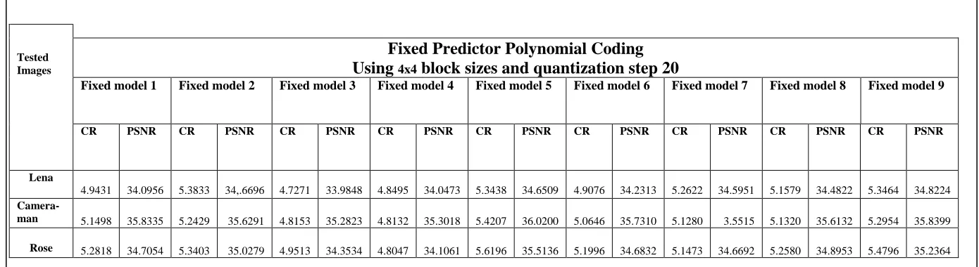
The result of the proposed compression system indicates that the high image quality is achieved because of utilization of effective fixed predictor coding technique along with the efficient linear polynomial coding technique. The results showed in table (2) of block sizes 4×4. It is obvious that the blocks size and the quantization step affected the technique performance, where the quantization process utilized for the linear polynomial model, so

the quantization levels of the coefficients and the residual affects the image quality and compression ratio. Figure (5) illustrated the results of the

Qa1,Qa2={1,2,2} and quantization level of residual

equal to {20}.

IV. CONCLUSIONS

The results affected by image details or characteristics, that implicitly direct affected the predictor selection as shown in Figure (5), where for Lena image (detailed or complex image) all the predictors were used, but to various degrees of occurrence; there was no concentration on specific predictors, while for the image with simpler detail (Camera-man and Rose), however, we found the predictors being mainly concentrated on three specific predictors of index numbers of 1, 5 9, and 1,2,5, respectively, which is simple and not complicated, with little reliance on the others, so there was no need to incorporate all the predictors.

ACKNOWLEDGMENT

The heading of the Acknowledgment section and the References section must not be numbered.

Causal Productions wishes to acknowledge Michael Shell and other contributors for developing and maintaining the IJETT LaTeX style files which have been used in the preparation of this template. To see the list of contributors, please refer to the top of file IJETT Tran.cls in the IJETT LaTeX distribution.

REFERENCES

[1] Abdulah, A. Al-H. 2018. Hierarchal Polynomial Coding of Grayscale Lossless Image Compression. Diploma, Dissertation, Baghdad University, Collage of Science. [2] Ghadah, Al-K. 2012. Intra and Inter Frame Compression

for Video Streaming, Ph.D. Thesis, Dept. Computer Science.

[3] Rasha, Al-T. 2015. Intra Frame Compression Using Adaptive Polynomial Coding .MSc. thesis, Baghdad University, Collage of Science.

[4] Noor, S. M. 2015. Image Compression based on Adaptive Polynomial Coding. Diploma, Dissertation, Baghdad University, Collage of Science.

[5] George, L. E., and Ghadah, Al-K. 2015. Image Compression based on Non-Linear Polynomial Prediction Model. International Journal of Computer Science and Mobile Computing, 4(8), 91-97.

[6] Maha, A. Rajab, Ghadah, Al-K., and Ahmed, I. A. 2016. Hybrid Image Compression and Transmitted using MC-CDMA System. Iraqi Journal of Science, 57(3A), 1819-1832

[7] Ghadah, Al-K., Taha, M., and Salam, A. 2017. Correlated Hierarchal Autoregressive Models Image Compression. Diyala Journal for Pure Sciences. 13(3), 1-14.

[8] Ghadah, Al-K., and Noor, E. 2017. Medical Image Compression using Hybrid Technique of Wavelet Transformation and Seed Selective Predictive Method. International Journal of Engineering Research and Advanced Technology, 3(9), 1-7.

[9] Ghadah, Al-K. 2013. Image Compression based on Quadtree and Polynomial. International Journal of Computer Applications, 76(3),31-37.

[10] Ghadah, Al-K. and George, L. E..2013. Fast Lossless Compression of Medical Images based on Polynomial. International Journal of Computer Applications, 70(15), 28-32.

[11] Ghadah, Al-K and Hazeem, Al-K, 2014. Medical Image Compression using Wavelet Quadrants of Polynomial Prediction Coding & Bit Plane Slicing. International Journal of Advanced Research in Computer Science and Software Engineering, 4(6), 32-36.

[12] Ghadah, Al-K., and Maha, A. 2016. Lossless and Lossy Polynomial Image Compression. IOSR Journal of Computer Engineering (ISO-JCE), 18(4), 56-62.

[13] Ghadah, Al-K. and Noor, S. M. 2016. Image Compression based on Adaptive Polynomial Coding of Hard & Soft Thresholding. Iraqi Journal of Science, 57(2B), 1302-1307. [14] Ghadah, Al-K,. and Sara, A. 2017. The Use of First Order Polynomial with Double Scalar Quantization for Image Compression. International Journal of Engineering Research and Advanced Technology, 3(6), 32-42. [15] Ghadah, Al-K. and Rafaa, Y. 2017. Lossy Image

Compression Using Wavelet Transform, Polynomial Prediction and Block Truncation Coding. IOSR Journal of Computer Engineering (IOSR-JCE), 19(4),34-38.

Table (1): The Fixed Predictor Models [2].

Description

Predictor

FM

(1,cusal,1D)=

P(i,j-1)

S

a (left neighbor)

FM(

1,cusal,1D)=

P(i-1,j)

S

b(bottom neighbor)

FM

(1,cusal,1D)=

P(i-1,j-1)

S

c(left-bottom neighbor)

FM

(1,cusal,1D)=

P(i-1,j+1)

S

d(right-bottom neighbor)

FM

(2,cusal,2D)=

P((i,j-1)+P(i-1,j))/2

(S

a

+S

b

)/2

(average1)

FM

(2,cusal,2D)=

P(i,j-1)+(P(i,j-1)-P(i-1,j)/2)

S

a

+(S

a

-S

b

) /2)

(average2)

FM

(2,cusal,2D)=

P(i-1,j)+( P(i-1,j+1)- P(i-1,j)/2)

S

b

+(S

d

-S

b

)/2)

(average3)

FM

(2,cusal,2D)=

P(i-1,j)+(P(i,j-1)- P(i-1,j)/2)

S

b

+(S

a

-S

b

)/2)

(average4)

FM

(4,cusal,2D)=

P((i,j-1)+P(i-1,j)+ P(i-1,j-1)+ P(i-1,j+1))/2

(S

a

+S

b

+S

c

+S

d

)/4

ISSN: 2231-5381

http://www.ijettjournal.org

Page 185

S

c

S

b

S

d

S

a

S

X

S

e

S

f

S

k

S

u

S

q

S

y

S

z

S

t

Fig 3: Local Neighboring Pixels where The Predictors are Designed According to Table (1) Where Sx Refers to the Current Predicted Pixel,

Table (2): The Fixed Predictor Linear Polynomial Compression Performance of Compression Ratio and PSNR For Lena, Camera Man, and Rose Test Image Using Different 4x4 Block Sizes and Quantization Steps 20 of Residual (Error) And Coefficients

Tested Images

Fixed Predictor Polynomial Coding

Using

4x4

block sizes and quantization step 20

Fixed model 1 Fixed model 2 Fixed model 3 Fixed model 4 Fixed model 5 Fixed model 6 Fixed model 7 Fixed model 8 Fixed model 9

CR PSNR CR PSNR CR PSNR CR PSNR CR PSNR CR PSNR CR PSNR CR PSNR CR PSNR

Lena

4.9431 34.0956 5.3833 34,.6696 4.7271 33.9848 4.8495 34.0473 5.3438 34.6509 4.9076 34.2313 5.2622 34.5951 5.1579 34.4822 5.3464 34.8224

Camera-man 5.1498 35.8335 5.2429 35.6291 4.8153 35.2823 4.8132 35.3018 5.4207 36.0200 5.0646 35.7310 5.1280 3.5515 5.1320 35.6132 5.2954 35.8399

ISSN: 2231-5381

http://www.ijettjournal.org

Page 189

Fig 5: Index Residual Image and the Index of the Predictors For 4×4 Block for the Three Tested Images (A) Lena, (B) Camera-Man and (C) Rose, Where Each Block in that Image Shows Us The Index That Gives The Lowest Residual