Spatial based Expectation Maximizing (EM)

R E S E A R C H

Open Access

Spatial based Expectation Maximizing (EM)

M A Balafar

Abstract

Background:Expectation maximizing (EM) is one of the common approaches for image segmentation.

Methods:an improvement of the EM algorithm is proposed and its effectiveness for MRI brain image segmentation is investigated. In order to improve EM performance, the proposed algorithms incorporates neighbourhood information into the clustering process. At first, average image is obtained as neighbourhood information and then it is incorporated in clustering process. Also, as an option, user-interaction is used to improve segmentation results. Simulated and real MR volumes are used to compare the efficiency of the proposed

improvement with the existing neighbourhood based extension for EM and FCM.

Results:the findings show that the proposed algorithm produces higher similarity index.

Conclusions:experiments demonstrate the effectiveness of the proposed algorithm in compare to other existing algorithms on various noise levels.

Keywords:Em, Segmentation, Neighbourhood

1. Background

The application of image processing techniques for medical imaging process rapidly increases. Most medical images are stored and represented in softcopy [1]. Ultrasound, X-ray computed tomography, digital mammography and mag-netic resonance imaging (MRI) are the most common medical imaging types [2]. MRI can give different grey level for different tissues and various types of neuropathology if its acquisition parameters are adjusted [3].

Data acquisition, processing and visualization techni-ques facilitate diagnosis. Medical image segmentation plays a very important role in many computer-aided diagnostic tools. These tools could save clinicians’time by simplifying complex time-consuming processes [4]. The main part of these tools is to design an efficient seg-mentation algorithm. Medical images mostly contain unknown noise [5], in-homogeneity [6] and complicated structures. Therefore, segmentation of medical images is a challenging and complex task. Medical image segmen-tation has been an active research area for a long time. There are many segmentation algorithms but there is no generic algorithm for a totally successful segmentation of medical images [7].

Clustering methods are common for MRI brain segmen-tation. Expectation-maximization (EM) and fuzzy c-mean (FCM) are the most popular clustering algorithms. The Gaussian mixture model (GMM) is a popular segmenta-tion method. EM is used to estimate the parameters of this model. FCM and EM only consider the intensity of images and in noisy images, intensity is not trustful [8-10]. Usually, spatially adjacent pixels belong to the same clus-ter. Many algorithms introduced to make FCM [11-17] and EM robust against noise but nevertheless most of them were and are flawless to some extent. Usually, spa-tially adjacent pixels belong to the same cluster. Many researchers attempted to incorporate spatial information into FCM and EM to overcome the noise problem. Zhang et. al. [18] proposed a novel Gaussian hidden Markov Random Field (HMRF) model to integrate spatial informa-tion into Gaussian model. They used a Markov Random Field-Maximum A Posteriori (MRF-MAP) approach to estimate the model solution. Recently, Tang et al. [19] proposed a neighbourhood-weighted Gaussian mixture model to overcome misclassification on the boundaries and on inhomogeneous regions of MRI brain images with noise. A. R. F. d. Silva [20] proposed two Bayesian algo-rithms (DPM, rjMCMC) which use Markov chain sam-pling techniques to find normal mixture models with an unknown number of components. They used algorithms for MRI segmentation and compared performance of their Correspondence: [email protected]

Dept of IT, Faculty of Electric and Computer, University of Tabriz, Tabriz, East Azerbaijan, Iran

algorithms with published results for two exist Bayesian based MRI brain segmentation methods (KVL [21], MPM-MAP [22]).

González Ballester et al. [23] and Tohka et al. [24] reported a statistical models namely a novel trimmed minimum covariance determinant (TMCD) for the esti-mation of the parameters of partial volume models to address partial volume averaging.

In order to make Gaussian mixture model more robust against complex tissue spatial layout, Greenspan et al. [25] proposed the parameter-tied, constrained Gaussian ture model (CGMM) to capture this problem. The mix-ture model composed of a large number of Gaussians for each tissue is used to capture the complex tissue spatial layout. The Gaussian parameters of a tissue are tied using intensity as global feature. The parameters are learned using the expectation-maximization (EM) algorithm.

In [26], a nonparametric Bayesian model, known as Dirichlet process mixture model (DPMM) is proposed to overcome the limitations of current parametric finite mix-ture models. The DPMM permits unknown number of components in the mixture and allow robust segmentation of brain with unknown or incomplete specifications.

In [27], local cooperative unified segmentation (LOCUS) approach based on distributed local MRF models for brain segmentation is presented. The volume is partitioned into

sub volumes and a set oflocalandcooperativeMarkov

random field (MRF) models are distributed. In order to ensure consistency, neighbour local MRFs are estimated cooperatively. The intensity in-homogeneity correction is not required due to precisely fit of Local estimation with the local intensity distribution.

In this paper, a new modification to GMM and EM is introduced by incorporating neighbourhood information into likelihood function and EM steps. The average of neighbour pixels around each pixel is calculated prior to GMM clustering and incorporated in GMM and EM func-tions beside the pixel value.

The rest of this paper is organized as follows. The stan-dard GMM model and EM segmentation algorithm are presented in Section 2.1. In Section 2.2, proposed modified EM algorithm is described. Also, improvement of segmen-tation results using use-interaction is presented in section 2.3. Experimental and comparison results are presented in Section 3 and this paper is concluded in Section 4.

2. Methods

A modification to GMM is introduced by incorporating neighbourhood information into likelihood function and EM steps.

2.1 Standard GMM

The Gaussian mixture model assumesM mixed

compo-nent densities (Gaussian distribution) for each pixel

(voxel) withM mixing coefficients. Each component is

assigned to one target class and the goal is to obtain the class probabilities of each pixel (voxel). The probability distribution of thejth component is denoted bypj(xi|θj),

wherexiis pixeliin input image andθjis the parameter

(meanμ_jand covariance matrix∑_j) of componentj. The probability distribution each pixel (voxel) can be described as a mixture of probability distributions as follows:

p(xi|θ) =

M

j=1

αjpj(xi|θj)

= 1

det(2πj)

e−(x−μj)Tj−1(x−μj)/2

(1)

Where aj denotes the mixture coefficient with the

constraint,

M

j=1

αj= 1 The probability distribution of

component j is modelled by a Gaussian distribution

with meanμjand covariance matrix∑j:

pj(xi|θj) =pj(xi|μj,j) (2)

Usually, maximum likelihood (ML) estimation is used to find the parameters. The log-likelihood expression for the parameterθand the image Xis defined as follows:

log(L(θ|X)) = log

N

i=1 p(xi|θ)

= N i=1 log( M j=1 αt

jpj(xi|θjt))

(3)

Finding the ML solution from this equation is difficult. Usually, the expectation-maximization (EM) is used to obtain the parameters. EM steps are demonstrated in the following:

E-step. Bayes’rule is used to obtain the probability of datax_ibelong to classθ_j(E-step):

p(j|xi,θt) = α

t

jpj(xi|θjt) M

j=1α t

jpj(xi|θjt)

(4)

M-step. Probability obtained in E-step is used to obtain mixing coefficient, mean and covariance matrix (M-step):

αt+1 j = 1 N N i=1

μt+1 j =

N

i=1

xip(j|xi,θt₎

N

i=1

p(j|xi,θt₎

(6) t+1 j = N i=1

p(j|xi,θt_).(xi−μt+1

j )(xi−μtj+1) T

N

i=1

p(j|xi,θt₎

(7)

c. EM steps are repeated until convergence.

2.2. Modified GMM

The average of neighbour pixels around xi¯ is calculated prior to GMM clustering. In the likelihood function (Equation 3), distribution value of xi¯ is added to the dis-tribution value of pixel xias neighbourhood information:

log(L(θ |X)) = log

N

i=1

p(xi|θ) =

N i=1 log( M j=1 αt

j[(1−β)∗pj(xi|θjt) +β∗pj(¯xi|θjt)])

(8)

The parameterbdetermines the weight of

neighbour-hood information. Incorporating neighbourneighbour-hood infor-mation improves the performance of segmentation methods in high level of noise, but the blurring effect degrades the performance of them in low noise level. In order to overcome the degrading effect of algorithms in low level of noise, the variance of noise is used to spe-cify the weight of neighbourhood information (b). Its value is set tos, wheres is the variance of noise. In previous neighbourhood based EM extensions, neigh-bourhood information is calculated in clustering

itera-tion; but in this algorithm x¯i is computed before

iteration, thus, the clustering will be faster. An extension of EM named EM-1 is introduced to solve likelihood function. The EM is modified as follows:

a. In Equation 4, distribution value of x¯i is added to the

distribution value of pixel xias neighbourhood informa-tion:

A= [(1−β)∗pj(xi|θ_jt) +β∗pj(xi¯ |θ_jt)]

p(j|xi,θt) = α

t j.A

j=1 αt

j.A

(9)

b. In Equation 6, xi¯ is added to x_i as neighbourhood information:

μt+1 j =

N

i=1

((1−β)∗xi+β∗ ¯xi)p(j|xi,θt₎

N

i=1

p(j|xi,θt₎

(10)

c. In Equation 7, the distance of xi¯ from the compo-nent centre is added to the distance ofxifrom the

com-ponent centre as neighbourhood information:

d(x) = (x−μ_jt+1)(x−μt_j+1)T

t+1 j =

N

i=1

p(j|xi,θt_{).(d(xi) +β.d(xi¯))}

N

i=1

p(j|xi,θt₎

(11)

In MRI, noise behaves as Rician distributed noise. Rician noise approaches Gaussian distribution in high Signal to Noise Ratio (SNR) and Rayleigh distribution in low SNR [28]. Rician distribution in the background is Rayleigh because there is no signal. The Rayleigh PDF of the statistically independent observations is

p({Oi}) =

n

i=1 Oi σ2e

−(O2

i)/(2σ2) ₍₁₂₎

Where Ois observations and σ_Noise2 is the variance of noise. The variance of noise is obtained by maximizing the log-likelihood of PDF function with respect to var-iance: σ2 Noise= 1 2n n i=1

O2_i (13)

In other words, background pixels are considered as observations (O) and the variance of noise is obtained applying equation 13 on background pixels values. For that, the powers of background pixels values are com-puted and half of the average of resulted values is con-sidered as variance of the noise.

Also, in-homogeneity correction [6] is applied to input image with in-homogeneity pollution and the propose GMM is applied on in-homogeneity corrected image.

2.3. Improving Segmentation Results Using User Interaction

Sometimes, due to in-homogeneity, low contrast, noise and inequality of content with semantic, automatic meth-ods fail to segment image correctly. Therefore, for these images, it is necessary to use user interaction to correct

method’s error [29]. However, robust semi-automatic

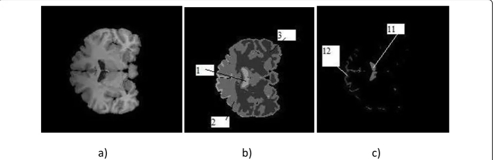
Sometimes, segmented image, for example in Figure 1 (b), either has pixels from two or more tissues in one clus-ter (csf and grey matclus-ter of brain in clusclus-ter number 2) or pixels from one tissue in two or more clusters(white mat-ter in clusmat-ters number 2 and 3). For solving this problem, user selects clusters contain several tissues (cluster num-ber 1) to be re-clustered to two sub clusters. Figure 1(c) demonstrates sub clusters of class number 1. The cluster number 1 is clustered to two sub clusters number 11 and 12.

This process continues until user is satisfied. That means quality of segmentation depends on user. Then, to solve problem of several clusters for one tissue, user selects clusters for each tissue (clusters 12 is also selected for grey matter). Steps of this method listed as follow:

1. Input volume is clustered to the n clusters where n is the number of target class (tissues). The output is clustered volume.

2. Under segmentation: If some clusters contain more than one target class (tissue), user selects such clus-ters to be partitioned more; each user selected cluster is re-clustered to two sub clusters. This process con-tinues till user is satisfied. The output is clustered volume without under segmentation.

3. Over segmentation: If several clusters correspond to one target class (tissue), user selects clusters for each target class. The output is final clustered volume.

3. Experimental Results and Discussion

The proposed extension of EM (EM-1) and the existing neighbourhood-based extension of EM [19] (referred as NWEM in this paper for clear understanding) are simu-lated and tested on the simusimu-lated volumes from BrainWeb [30] and real volumes from Internet Brain Segmentation Repository (IBSR) [31].

Moreover, reported results on simulated volumes for existing extensions of EM (DPM, rjMCMC, KVL, MPM-MAP) and existing neighbourhood based extension for FCM (FCM_S [32], FCM_EN [33], FGFCM [34], FLICM [35] and NonlocalFCM [36]) are used to evaluate pro-posed algorithm.

Also, the reported results on real volumes from IBSR are used to evaluate proposed algorithms. Furthermore, mentioned FCM extensions simulated and tested on real volumes.

The results of algorithms are compared quantitatively to analyse their performance. The neighbourhood size,N for proposed algorithm is set to 3 × 3. Three indices (similarity index, false positive ratio and false negative ratio) [37] are used to evaluate the algorithms quantita-tively. The similarity indexriof class i is the degree of

the class pixels matching between ground truth and seg-mentation result for the same class. The false positive ratiorfp represents extra pixels of classiand the false negative ratiorfn represents lost pixels of classi. They are defined as follows:

ρi=

2|Xi∩Yi|

|Xi|+|Yi| rf pi=

|Yi| − |Xi∩Yi|

|Xi| rf ni=

|Xi| − |Xi∩Yi| |Xi| (14)

where X_i represents classi in ground truth andY_i

represents the same class in the segmentation result. Each index for full segmentation results is the average of that index for all classes.

3.1. Simulated volumes

The simulated MRI volumes are obtained from Brain-Web. A simulated data volume with T1-weighted sequence, slice thickness of 1 mm and a volume size of 217 × 181 × 181 is used. Non-brain tissues are removed prior to segmentation.

The number of tissue classes in the segmentation is set to three: grey matter (GM), white matter (WM) and cerebrospinal fluid (CSF). All pixels in the image are

a)

b) c)

contributed in segmentation process but in evaluation process, background pixels are ignored following pre-vious works utilized in this paper. In the public data-bases which have been used in the paper and generally in brain MRI volumes, background pixels have black value. Therefore, cluster with lowest average grey value is considered as background.

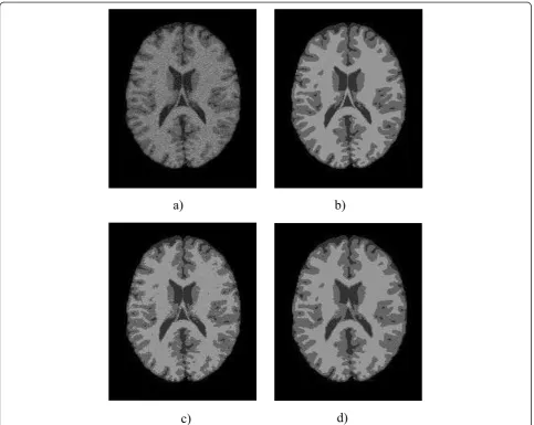
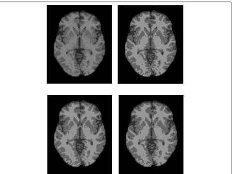
First, EM-1 and NWEM were applied to a slice of T1-weighted brain image corrupted by different noise levels. Figure 2 and Figure 3 show the segmentation results of applying the afore-mentioned algorithms on a T1-weighted normal brain slice in the presence of 9% and 7% rician noise, respectively.

The segmentation results of white matter (WM), grey matter (GM) and cerebrospinal fluid (CSF) are depicted in. (a) is noisy image. (b) is ground-truth. (c) to (d) are the segmentation results of NWEM and EM1, respectively.

From the above qualitative comparison, it was not dif-ficult to find that NWEM was more influenced by the

noise in comparison with EM1, in which fewer artefacts were evident, resulting in clearer segmentation result.

Also, the proposed segmentation algorithm (EM-1) and NWEM are applied to brain volume and average similarity value is used to evaluate them. Figure 4 shows the average similarity indexesrof mentioned algorithms in different noise levels.

Figure 4 shows that EM-1 produces higher similarity indexes and lower rfp and rfn, meaning that this algo-rithm produces more accurate segmentation results. The similarity index of EM-1 decreases more slowly than NWEM algorithm when noise level increases. In the same time, the rfp and rfn of EM-1 increases faster than NWEM algorithm.

Both algorithms give similar results, under 5% noise level. However, for more than 5%, EM-1 exhibits much better results than the NWEM algorithm. Incorporating average of neighbourhood information, in clustering process of NWEM, make this algorithm robust against

a)

b)

c)

d)

noise but has blurring as side effect. It seems that with increasing noise level more than 5% noise level; this incorporation cannot overcome high level of noise.

Also the effect of different neighbourhood sizes on performance of proposed segmentation algorithm (EM-1) is investigated. Figure 5 shows the average similarity

indexr of EM-1 for different neighbourhood sizes on

volume with 9% noise. Figure 5 shows that when the neighbourhood size is increased, the similarity index of EM-1 decreases sharply. This means blurring effect in EM-1 depends on neighbourhood size.

The speed of EM1 and NWEM in segmenting a slice was also investigated. Figure 6 represents the average time required to segment a slice using the mentioned algorithms. Figure 6 shows that EM1 is faster than NWEM. The neighbourhood information in NWEM is calculated in NWEM clustering iteration. Therefore, it is time-consuming.

The proposed segmentation algorithm is also compared with current extensions for EM. The average similarity

indexesrfor proposed algorithm (EM-1) and several

current extensions for EM (DPM, rjMCMC, KVL and MPM-MAP) are shown in Figure 7. Figure 7 shows that EM-1 produces highest similarity indexes. The proposed segmentation algorithm gives results comparable with the best reported results, in low level of noise. However, for noise levels more than 5%, EM-1 algorithm outper-form other competing algorithms and this difference in performance gets more in 9% noise level.

Also, EM-1 is compared with current existing neigh-bourhood based extensions for FCM. Figure 8 shows the average similarity indexesrfor EM-1 and FCM extensions (FCM_S, FCM_S1, FCM_EN, FGFCM and FLICM) in dif-ferent noise levels. At 3% noise level, the results for pro-posed segmentation algorithm and the best reported result were close. Above 3% noise, EM-1 produces higher simi-larity index and were the most convincing in segmenta-tion. The superiority of these algorithms increases with increasing in noise level. FLICM shows worst performance it seems it is not suit algorithm for brain volumes.

In [25], the parameter-tied, constrained Gaussian mix-ture model (CGMM) is applied on image volume from brainweb with different noise levels. Average similarity index for different algorithms with variant noise levels (3%, 5%, 7%, 9%) are: CGMM (0.93, 0.93, 0.92 and 0.895) and KVL (0.925, 0.915, 0.895 and 0.865). The proposed segmentation algorithm outperforms KVL and CGMM.

3.2. Real volumes

The superiority of our algorithm is also demonstrated on real MRI volumes. The real MRI volumes are obtained from the IBSR by the Centre for Morphometric Analysis at Massachusetts General Hospital. 20 normal data

volume with T1-weighted sequence are used. First, pro-posed algorithm (EM-1) is applied to slices of a real MRI volume with size 256*256*53. The average similarity

indexrfor volume image is 0.7986. Figure 9 shows the

similarity indexes of proposed algorithm (EM-1) for each slice of MRI volume. In almost all slices, the proposed algorithms exhibit better results for WM in compare to results for GM. Better performance of proposed algo-rithms in WM is due to more simplicity and compactness of WM in compare to GM.

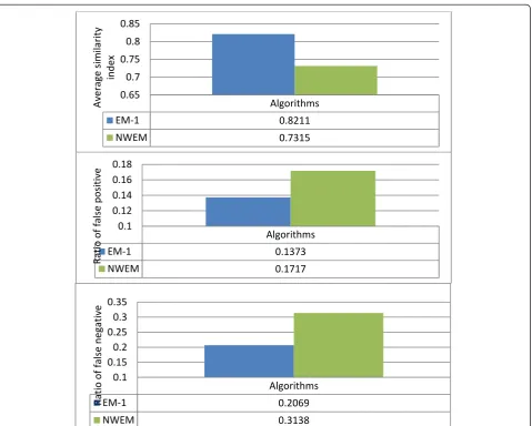
EM-1 and NWEM are applied to all 20 normal real MRI volumes and average similarity indexris used to compare the segmentation results, quantitatively. Figure 10 shows

3% 5% 7% 9%

EM1 0.9604 0.949 0.938 0.93

NWEM 0.9624 0.9489 0.931 0.91 0.9

0.91 0.92 0.93 0.94 0.95 0.96 0.97

Similarity index

Noise level

3% 5% 7% 9%

EM1 0.0356 0.051 0.0698 0.0684 NWEM 0.0322 0.0509 0.0733 0.0989

0 0.02 0.04 0.06 0.08 0.1 0.12

Ratio of

false

positive

Noise level

3% 5% 7% 9%

EM1 0.0386 0.0472 0.0497 0.0589 NWEM 0.0425 0.0546 0.0694 0.0922

0.03 0.04 0.05 0.06 0.07 0.08 0.09

Ratio of

false

negative

Noise level

the average similarity index, rfp and rfn values of both algorithms for all 20 normal volumes. Figure 10 shows that EM-1 outperforms NWEM. EM-1 produces higher average similarity indexesrand lower rfp and rfn.

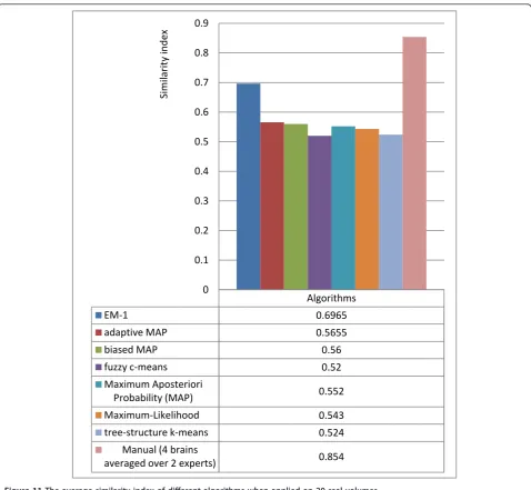
The average similarity index values of proposed algo-rithm for 20 normal real MRI volumes and EM exten-sions (reported results in IBSR) are compared. Figure 11 shows the average similarity index values of different algorithms for all 20 normal volumes. Figure 11 shows that the similarity index for proposed segmentation algorithms is higher than competing methods. It can be seen clearly that proposed algorithm has a better perfor-mance over reported results, meaning that proposed algorithm produces more accurate segmentation results

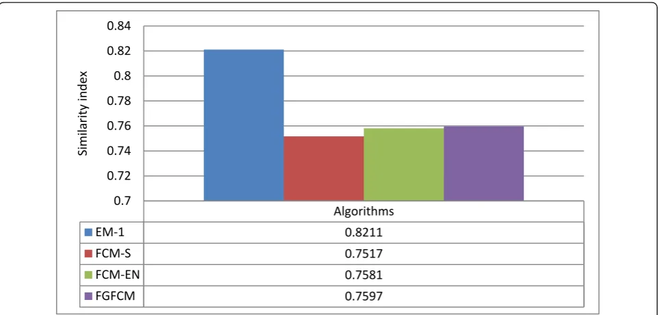
The proposed algorithms are also compared with neighbourhood based extensions for FCM. Figure 12

shows the average similarity indexes r for proposed

algorithm and FCM extensions (FCM_S1, FCM_EN, FGFCM) for all 20 normal volumes.

It can be seen clearly that proposed algorithm has a better performance over FCM extension methods, and

produces more accurate segmentation results. FCM extensions also incorporate neighbourhood information in FCM clustering process, but, it seems that incorporat-ing neighbourhood information improves EM more than FCM method.

In [24], a novel trimmed minimum covariance deter-minant (TMCD) method an extension for Gaussian mix-ture model is applied on 20 normal image volumes from IBSR. The average jaccard value was 0.6722. The average jaccard values for EM-1 is: 0.695. The similarity index for EM-1 is higher than reported result, meaning that EM-1 produces more accurate segmentation results.

In [25], the parameter-tied, constrained Gaussian mixture model (CGMM) is applied on 18 volumes from 20 normal image volumes (except volume 4-8 and 202-3) in IBSR website. The CGMM results is compared with reported results from the IBSR website, as well as with the Marroquin algorithm [38]. Marro-quin’s algorithm is an atlas-based Bayesian segmenta-tion algorithm. The CGMM algorithm outperforms other studied methods. Jacc similarity index CGMM

3 5 7

EM1 0.93 0.8674 0.7935

0.7 0.75 0.8 0.85 0.9 0.95

Similarity index

Neighbourhood size

Figure 5The average similarity indexrfor different neighbourhood sizes on simulated volume with 9% noise.

0 0.5 1 1.5 2 2.5 3 3.5 4 4.5

Average time

(secon

d)

Algorithms

EM1

NWEM

3% 5% 7% 9%

EM1 0.9604 0.949 0.938 0.93

DPM 0.942 0.927 0.902 0.894

rjMCMC 0.92 0.897 0.882 0.875

KVL 0.922 0.923 0.901 0.874

MPM-MAP 0.955 0.942 0.905 0.875

0.84 0.86 0.88 0.9 0.92 0.94 0.96 0.98

Similarity index

Noise level

Figure 7The average similarity indicesrfor different noise levels.

3% 5% 7% 9%

EM-1 0.9604 0.9485 0.938 0.93

FCM-S 0.9505 0.9307 0.914 0.901

FCM-EN 0.94 0.933 0.9298 0.918

FGFCM 0.9505 0.9308 0.915 0.89

NOnlocalFCM 0.9605 0.9402 0.9203 0.9106

FLICM 0.8677 0.8492 0.8223 0.7854

0.78 0.8 0.82 0.84 0.86 0.88 0.9 0.92 0.94 0.96 0.98

Similarity index

Noise level

Figure 9The similarity index of proposed algorithm when applied for real volume.

Algorithms

EM-1 0.8211

NWEM 0.7315

0.65 0.7 0.75 0.8 0.85

Average similarity

index

Algorithms

EM-1 0.1373

NWEM 0.1717

0.1 0.12 0.14 0.16 0.18

Ratio

of false positive

Algorithms

EM-1 0.2069

NWEM 0.3138

0.1 0.15 0.2 0.25 0.3 0.35

Ratio

of false negative

was: 0.67. The average jaccard values for EM-1 is: 0.6971. EM-1 outperforms the best reported result which is for CGMM.

In [26], a nonparametric Bayesian model, known as Dirichlet process mixture model (DPMM) is applied on 13 volumes (1_24, 2_4, 5_8, 6_10, 7_8, 11_3, 12_3, 13_3, 15_3, 16_3, 100_23, 110_3 112_2) from the 20 normal T1-weighted brain image volumes from IBSR. The similarity index for DPMM is higher than competing methods. Dice similarity index for DPMM was: 0.7071. The proposed algorithms are applied on the same volumes. The average Dic value for EM-1 is: 0.8219. The similarity index for pro-posed method is higher than the best reported result which is for DPMM, meaning that proposed method are the most convincing in segmentation.

In [27], local cooperative unified segmentation (LOCUS) approach which is based on distributed local MRF models for brain segmentation is applied on the 20 normal T1-weighted brain image volumes from IBSR. LOCUS-T is compared with published results for SPM5 and FAST. Dic similarity index for different methods are: LOCUS-T = 0.765, SPM5 = 0.81, FAST = 0.765. The average Dic value for EM-1 is: 0.8211. EM-1 out-performs the best reported result which is for SPM5.

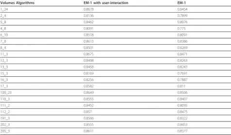
Also, improvement of segmentation result using user-interaction is investigated. Proposed algorithms and the same algorithm with user-interaction are applied to all 20

normal real MRI volumes and similarity indexris used

to compare the segmentation results, quantitatively. The average similarity index values of both algorithms for

Algorithms

EM-1 0.6965

adaptive MAP 0.5655

biased MAP 0.56

fuzzy c-means 0.52

Maximum Aposteriori

Probability (MAP) 0.552

Maximum-Likelihood 0.543

tree-structure k-means 0.524

Manual (4 brains

averaged over 2 experts) 0.854

0 0.1 0.2 0.3 0.4 0.5 0.6 0.7 0.8 0.9

Similarity index

different volume were presented in Figure 13 and Table 1. Figure 13 shows that user-interaction improves perfor-mance of proposed algorithm and increases similarity indexesrin all image volumes.

4. Conclusion

In this paper, an extension of EM has been introduced. In order to overcome the problem of standard EM in the pre-sence of noise, the introduced algorithms are formulated by modifying the equations of the standard EM algorithm which allow the neighbourhood pixels to be incorporated in the labelling of a pixel. Introduced algorithm is tested

on simulated MRI volumes, with different noise levels and real volumes. The performance of the existing neighbour-hood based EM and FCM algorithms and proposed algo-rithm are compared qualitatively.

The similarity index, r is used to evaluate different algorithms. Experiments demonstrate the effectiveness of the proposed algorithm in compare to other existing algorithms on various noise levels in terms of similarity index,r.

In future, we consider doing research on other kinds of segmentation methods to improve their functional-ities. Also, we will analyse the effects of different

0.6 0.65 0.7 0.75 0.8 0.85 0.9

1_24 2_4 5_8 4_8 6_10 7_8 8_4 11_3 12_3 13_3 15_3 16_3 17_3

100_23 110_3 111_2 112_2 191_3 202_3 205_3

Similarity index

Volumes

EM-1 with user-interaction

EM-1

Figure 13The similarity index of different algorithms when applied on 20 real volumes. Algorithms

EM-1 0.8211

FCM-S 0.7517

FCM-EN 0.7581

FGFCM 0.7597

0.7 0.72 0.74 0.76 0.78 0.8 0.82 0.84

Similarity index

clustering methods in segmentation of medical images for the diagnosis of abnormal or various important mat-ters in medical images.

Authors_’contributions

MA performed all works for this paper.

Competing interests

The authors declare that they have no competing interests.

Received: 10 June 2011 Accepted: 26 October 2011 Published: 26 October 2011

References

1. Chang PL, Teng WG:“Exploiting the self-organizing map for medical image segmentation”.Twentieth IEEE International Symposium on Computer-Based Medical Systems2007, 281-288.

2. Jan J:Medical image processing, reconstruction, and restoration: concepts and methods: CRC2006.

3. Tian D, Fan L:_“A Brain MR Images Segmentation Method Based on SOM Neural Network”.The 1st International Conference on Bioinformatics and Biomedical Engineering2007, 686-689.

4. Jiang Y, Meng J, Babyn P:“X-ray image segmentation using active contour model with global constraints”.2007, 240-245.

5. Balafar MA:“New spatial based MRI image de-noising algorithm”.Artifitial Intelligence Review2011, 1-11.

6. Balafar MA, Ramli AR, Mashohor S:“A New Method for MR Grayscale Inhomogeneity Correction”.Artificial Intelligence Review, Springer2010,

34:195-204.

7. Balafar MA, Ramli AR, Saripan MI, Mashohor S:“Review of brain MRI image segmentation methods_”.Artificial lntelligence Review2010,33:261-274. 8. Balafar MA, Ramli AR, Mashohor S:“Compare different spatial based Fuzzy

C-Mean (FCM) extensions for MRI Image Segmentation_”.ICCAE2010, 609-611.

9. Balafar MA, Ramli AR, Mashohor S:_“Edge-preserving Clustering Algorithms and Their Application for MRI Image Segmentation”.International MultiConference of Engineers and Computer Scientists2010, 17-19. 10. Balafar MA, Ramli A-R, Mashohor S:“Medical Brain magnetic resonance

image segmentation using novel improvement for expectation maximizing”.Neurosciences2011,16:242-247.

11. Balafar MA, Ramli AR, saripan MI, Mashohor S, Mahmud R:“Improved Fast Fuzzy C-Mean and its Application in Medical Image Segmentation”. Journal of Circuits, Systems, and Computers2010,19:203-214.

12. Zou K, Wang Z, Hu M:_“An new initialization method for fuzzy c-means algorithm”.Fuzzy Optimization and Decision Making2008,7:409-416. 13. Chuang K-S, Tzeng H-L, Chen S, Wu J, Chen T-J:_“Fuzzy c-means clustering

with spatial information for image segmentation”.Computerized Medical Imaging and Graphics2006,30:9-15.

14. He R, Datta S, Sajja BR, Narayana PA:“Generalized fuzzy clustering for segmentation of multi-spectral magnetic resonance images”. Computerized Medical Imaging and Graphics2008,32:353-366.

15. Balafar MA, Ramli AR, Saripan MI, Mashohor S, Mahmud R:“Medical Image Segmentation Using Fuzzy C-Mean (FCM) and User Specified Data_”. Journal of Circuits, Systems, and Computers2010,19:1-14.

16. Balafar MA, Ramli AR, Saripan MI, Mahmud R, Mashohor S:_“Medical image segmentation using fuzzy C-mean (FCM) and dominant grey levels of image_”.Visual information engineering conference2008, 314-317. 17. Balafar MA, Ramli AR, Saripan MI, Mahmud R, Mashohor S:“MRI

segmentation of medical images using FCM with initialized class centers via genetic algorithm”.International symposium on information technology

2008, 1-4.

18. Zhang Y, Brady M, Smith S:“Segmentation of brain MR images through a hidden Markov random field model and the expectation-maximization algorithm_”.IEEE Transactions on Medical Imaging2001,20:45-57. 19. Tanga H, Dillensegerb J, Baoa XD, Luoa LM:“A Vectorial Image Soft

Segmentation Method Based on Neighborhood Weighted Gaussian Mixture Model”.Computerized Medical Imaging Graphics2009,33:644-650. 20. Silva ARFd:_“Bayesian mixture models of variable dimension for image

segmentation”.computer methods and programs in biomedicine2009,

94:1-14.

Table 1 The similarity index of different algorithms when applied on 20 real volumes

Volumes Algorithms EM-1 with user-interaction EM-1

1_24 0.8678 0.8454

2_4 0.8136 0.7899

5_8 0.8462 0.8076

4_8 0.8091 0.775

6_10 0.8518 0.8091

7_8 0.8613 0.8386

8_4 0.8501 0.8269

11_3 0.8675 0.8471

12_3 0.8498 0.8263

13_3 0.8458 0.8243

15_3 0.8169 0.7691

16_3 0.8256 0.7887

17_3 0.8582 0.811

100_23 0.8649 0.8506

110_3 0.8555 0.8407

111_2 0.8452 0.8095

112_2 0.857 0.8475

191_3 0.8566 0.8322

202_3 0.8555 0.8453

21. Leemput FMKV, Vandermeulen D, Suetens P:“Automated model-based tissue classification of MR images of the brain_”.IEEE Transactions on Medical Imaging1999,18:897-908.

22. Marroquin BCVJL, Botello S, Calderon F, Fernandez-Bouzas A:_“An accurate and efficient Bayesian method for automatic segmentation of brain MRI_”.IEEE Transactions on Medical Imaging2002,21:934-945. 23. Ballester MG, Zisserman A, Brady M:“Estimation of the partial volume

effect in MRI_”.Medical Image Analysis2002,6:389-405.

24. Tohka J, Zijdenbos A, Evans A:“Fast and robust parameter estimation for statistical partial volume models in brain MRI”.NeuroImage2004,

23:84-97.

25. Greenspan H, Ruf A, Goldberger J:“Constrained Gaussian mixture model framework for automatic segmentation of MR brain images_”.IEEE transactions on medical imaging2006,25:1233-1245.

26. Silva ARFd:_“A Dirichlet process mixture model for brain MRI tissue classification”.Medical Image Analysis2007,11:169-182.

27. Scherrer B, Forbes F, Garbay C, Dojat M:_“Distributed Local MRF Models for Tissue and Structure Brain Segmentation”.IEEE TRANSACTIONS ON MEDICAL IMAGING2009,28:1278-1295.

28. Gudbjartsson H, Patz S:“The Rician distribution of noisy MRI data”. Magnetic resonance in medicine: official journal of the Society of Magnetic Resonance in Medicine/Society of Magnetic Resonance in Medicine1995,

34:910.

29. Balafar MA, Ramli AR, Saripan MI, Mahmud R, Mashohor S:_“Medical image segmentation using fuzzy C-mean (FCM), Bayesian method and user interaction_”.International conference on wavelet analysis and pattern recognition2008, 68-73.

30. ,_“BrainWeb [Online]: http://mouldy.bic.mni.mcgill.ca/brainweb/, Last accessed october, 2010.”.

31. ,“IBSR. Available: http://www.cma.mgh.harvard.edu/ibsr/, Last accessed october, 2010.”.

32. Ahmed MN, Yamany SM, Mohamed N, Farag AA, Moriarty T:“A modified fuzzy c-means algorithm for bias field estimation and segmentation of MRI data”.IEEE Transactions on Medical Imaging2002,21:193-199. 33. Szilágyi L, Benyó Z, Szilágyii SM, Adam HS:_“MR brain image segmentation

using an enhanced fuzzy c-means algorithm”.25th Annual International Conference of IEEE EMBS2003, 17-21.

34. Cai W, Chen S, Zhang D:“Fast and robust fuzzy c-means clustering algorithms incorporating local information for image segmentation”. Pattern Recognition2007,40:825-838.

35. Krinidis S, Chatzis V:“A Robust Fuzzy Local Information C-Means Clustering Algorithm”.IEEE Transactions on Image Processing2010,

19:1328-1337.

36. Wang J, Kong J, Lub Y, Qi M, Zhang B:_“A modified FCM algorithm for MRI brain image segmentation using both local and non-local spatial constraints_”.Computerized Medical Imaging and Graphics2008,32:685-98. 37. Zijdenbos AP, Dawant BM:“Brain segmentation and white matter lesion

detection in MR images_”.Crit Rev Biomed Eng1994,22:401-465. 38. Marroquin J, Vemuri B, Botello S, Calderon F, Fernandez-Bouzas A:“An

accurate and efficient Bayesian method for automatic segmentation of brain MRI”.IEEE Transactions on Medical Imaging2002,21:934-945.

doi:10.1186/1746-1596-6-103

Cite this article as:Balafar:Spatial based Expectation Maximizing (EM).

Diagnostic Pathology20116:103.

Submit your next manuscript to BioMed Central and take full advantage of:

• Convenient online submission

• Thorough peer review

• No space constraints or color figure charges

• Immediate publication on acceptance

• Inclusion in PubMed, CAS, Scopus and Google Scholar

• Research which is freely available for redistribution