Combinatorial Regression and Improved Basis Pursuit for Sparse Estimation

(1)

Pursuit for Sparse Estimation

Thesis by

M. Amin Khajehnejad

In Partial Fulfillment of the Requirements for the Degree of

Doctor of Philosophy

California Institute of Technology Pasadena, California

2012

(2)

c 2012

(3)

Acknowledgements

I would like to sincerely thank my adviser Dr. Babak Hassibi for his great sup-port of my research endeavors, and all my collaborators and coauthors including Dr. Salman Avestimehr (Cornell University), Dr. Alex Dimakis (University of Southern California), Dr. Amir Khojastepour (NEC Laboratories America Inc), Dr. William Bradley (Analog Devices/Lyric Labs), Dr. Benjamin Vigoda (Analog Devices/Lyric Labs), Dr. Weiyu Xu, Samet Oymak, Juhwan Yoo and Matthew Thill. I enjoyed collaboration with these smart people. I am also thankful to the members of my candidacy and defense talk committee, Professors Joel Tropp, Yaser Abu Mostafa, P. P. Vaidyanathan, Alex Dimakis and Tracy Ho for the insightful comments on this dissertation.

(4)

Abstract

Sparse representations accurately model many real-world data sets. Some form of sparsity is conceivable in almost every practical application, from image and video processing, to spectral sensing in radar detection, to bio-computation and genomic signal processing. Modern statistics and estimation theory have come up with ways for efficiently accounting for sparsity in enhanced information retrieval systems. In partic-ular, compressed sensing and matrix rank minimization are two newly born branches of dimensionality reduction techniques, with very promising horizons. Compressed sensing addresses the reconstruction of sparse signals from ill-conditioned linear mea-surements, a mathematical problem that arises in practical applications in one of the following forms: model fitting (regression), analog data compression, sub-Nyquist sampling, and data privacy. Low-rank matrix estimation addresses the reconstruc-tion of multi-dimensional data (matrices) with strong coherence properties (low rank) under restricted sensing. This model is motivated by modern problems in machine learning, dynamic systems, and quantum computing.

This thesis provides an in-depth study of recent developments in the fields of compressed sensing and matrix rank minimization, and sets forth new directions for improved sparse recovery techniques. The contributions are threefold: the design of combinatorial structures for sparse encoding, the development of improved recovery algorithms, and extension of sparse vector recovery techniques to other problems.

We propose combinatorial structures for the measurement matrix that facilitate compressing sparse analog signal representations with better guarantees than any of the currently existing architectures. Our constructions are mostly deterministic and are based on ideas from expander graphs, LDPC error-correcting codes and combi-natorial separators.

(5)

We propose novel reconstruction algorithms that are amenable to the combinato-rial structures we study, and have various advantages over the conventional convex optimization techniques for sparse recovery. In addition, we separately study the convex optimization Basis Pursuit method for compressed sensing, and propose reg-ularization schemes that expand the success domain for such algorithms. Our studies contain rigorous analysis, numerical simulations, and examples from practical appli-cations.

(6)

Combinatorial Structures for Sparse Recovery

30

2 Sparse Minimal Expanders 31 2.1 Introduction . . . 31

2.2 Related Work . . . 32

(7)

2.3 Contributions . . . 34

2.4 Preliminaries . . . 35

2.5 Analysis of`1 Minimization . . . 37

2.5.1 Null Space and Uniqueness Conditions . . . 37

2.5.2 Null Space of Adjacency Matrices . . . 40

2.6 Expander Graphs and Their Linear Algebraic View . . . 42

2.6.1 Perturbed Expanders . . . 45

2.6.2 Necessity of Expansion for Compressive Sensing . . . 47

2.7 Recovery Thresholds of Compressive Sensing for Minimal Expanders . 49 2.7.1 Strong Bound . . . 49

2.7.2 Weak Bound . . . 50

2.8 Fast Algorithm . . . 54

2.9 Experimental Evaluation . . . 55

2.10 Proof of Theorems . . . 57

2.11 Conclusion . . . 64

3 Bipartite Graphs with Large Girth 65 3.1 Introduction . . . 66

3.3.1 Compressed Sensing Preliminaries . . . 70

3.3.2 Channel Coding Preliminaries . . . 72

3.4 `1/`1 Guarantee for Ω(logn)-Girth Matrices . . . 74

3.4.1 Extension of CC-LPD . . . 75

3.4.2 Establishing the Connection . . . 81

4 Summary-Based Structures 85 4.1 Introduction . . . 87

4.5 Proposed Measurement Structures . . . 93

4.6 Practical Motivations . . . 94

4.6.1 Market Basket Analysis . . . 95

4.6.2 Wireless Ad-Hoc Networks . . . 97

4.7 Proposed Recovery Algorithms . . . 99

4.7.1 Basis Pursuit . . . 99

4.7.2 Summarized Index Recovery . . . 100

4.7.3 Mix and Match Algorithm . . . 103

4.8 Analysis . . . 103

4.8.1 `1 Minimization . . . 104

4.8.2 SIR Algorithm . . . 105

(8)

4.8.4 Recovery Bounds . . . 106

4.9 Simulations . . . 109

II

Threshold Improvement in Basis Pursuit

119

5 Compressed Sensing with Prior Information 120 5.1 Introduction . . . 122

5.4.1 Nonuniform Sparsity Model . . . 126

5.5 Summary of Main Results . . . 130

5.6 Derivation of the Results . . . 141

5.6.1 Upper Bound on the Failure Probability . . . 142

5.6.2 Special Case of Two Classes . . . 146

5.6.3 Generalizations . . . 151

5.6.4 Robustness To Noise . . . 153

5.7 Simulation Results . . . 154

6 Reweighted Basis Pursuit 165 6.1 Introduction . . . 166

6.5 Two-Step Weighted `1 Algorithm . . . 171

6.6 Approximate Support Recovery, Steps 1 and 2 of the Algorithm . . . 173

6.6.1 Scaling Law of `1 Minimization . . . 179

6.7 Perfect Recovery, Step 3 of the Algorithm . . . 180

6.8 Generalization to Beyond Gaussians . . . 183

6.8.1 Arbitrary Distributions . . . 184

III

Connections and Extensions of Methods

196

(9)

7.1 Introduction . . . 198

7.4 Extended Certificate and Robustness of LP Decoder . . . 206

7.5 Sufficient Conditions for LP Robustness . . . 209

7.5.1 Strong LP Robustness for Expander Codes . . . 210

7.5.2 Weak LP Robustness for Expander Codes . . . 212

7.5.3 Weak LP Robustness for Codes with Ω(log log(n)) Girth . . . 213

7.6 Implications of LP Robustness . . . 215

7.6.1 Mismatch Tolerance . . . 215

7.6.2 Pseudo-codewords and High-Error-Rate Subsets . . . 217

7.7 Iterative Reweighted LP Algorithm and Improved Threshold . . . 219

8 Matrix Rank Minimization 233 8.1 Introduction . . . 233

8.4 Rank Expanders and Proposed Operators . . . 238

8.4.1 Proposed Measurement Operator . . . 239

8.4.2 Existence of Rank Expanders . . . 239

8.5 Fast Recovery Algorithm . . . 242

8.6 Extension to Hermitians . . . 245

8.6.1 Expansion . . . 245

8.6.2 Recovery . . . 245

8.7 Simulation Results . . . 246

9 Future Work 248 10 Appendix 251 10.1 Elementary Bounds on Binomial Coefficients . . . 251

10.2 Hall’s Matching Theorem . . . 251

10.3 Restricted Isometry Property(RIP) . . . 252

10.4 RIP-1 for Expanders . . . 252

(10)

List of Figures

1.1 A pictorial demonstration of an under-determined system of linear equations acting on a sparse (compressible) vector . . . 4 1.2 Schematics of a sub-Nyquist sampling system . . . 7 1.3 Summary of existing categories of measurement matrices for compressed

sensing with examples . . . 14 1.4 Summary of existing categories of algorithms for compressed sensing

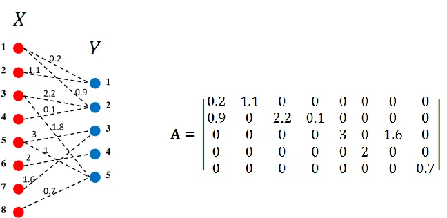
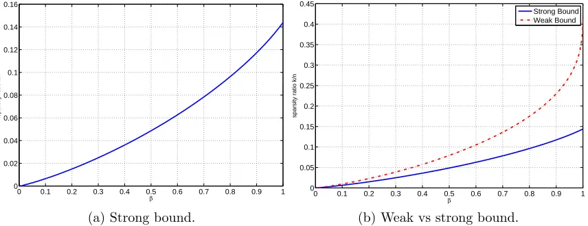
with examples . . . 16 2.1 A pictorial example of a (k, )-expander graph . . . 37 2.2 A weighted bipartite graph and its generalized adjacency matrix . . . 44 2.3 Recoverable sparsity size, weak achievable bound of Section 2.7.2 and the

strong achievable threshold of (2.7.1). β is the ratio m_n. . . 51 2.4 Comparison of weak and strong bounds for dense i.i.d. Gaussian matrices

(and nonnegative signals) from [DT05b] with those of the current paper for sparse matrices. β here is equal to m_n. . . 52 2.5 Comparison of size of recoverable sparsity (strong bound) of this paper with

those from [BGI+_08]. _β ₌ m

n. . . 53

2.6 (a) Probability of successful recovery of`1 minimization for a random

0₋1 sparse matrix of size 250_×500 with d= 3 ones in each column, and the same probability when the matrix is randomly perturbed in the nonzero entries. (b) Comparison of `1 minimization nonnegative

recovery, Algorithm 1, count-min algorithm of [CM04] and SMP algo-rithm of [BIR08] for sparse 0₋1 measurement matrices with dones in each column. _×: d = 3, _◦: d = 6, 2: d = 9. Blue: `1 minimization,

Black: Algorithm 1, Red: Count-min, Green: SMP . . . 56

(11)

2.7 Simulation results for Algorithm 1, noisy case; signal-to-error ratio vs. signal-to-noise ratio. . . 57 2.8 Decomposition of nodes and edges by Algorithm 1 . . . 62 3.1 Perturbed symmetric channel model . . . 74 3.2 The procedure of importing the performance guarantee from LP

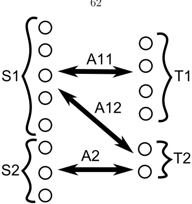
de-coding into compressed sensing . . . 74 4.1 An example (4,2) summary and the corresponding row of the

struc-tured measurement matrix . . . 94 4.2 An example of a measurement matrix constructed based on a (5,2)

summary codebook. Black is 1 and white is 0 . . . 94 4.3 An example of a measurement matrix of size 40_×32768 constructed

based on a random (15,2) summary codebook of size 40 . . . 95 4.4 Demonstration of a CS-based communication protocol in an ad-hoc

network . . . 98 4.5 Block diagram describing the subroutines of Algorithm 2 . . . 103 4.6 Required oversampling rate for successful recovery of Algorithm 2 on

proposed constructions versus signal dimension for various sparsity levels.110 4.7 Probability of successful recovery of Algorithm 2 versus sparsity level

k, for N = 32768 andM = 192,240,320,448 . . . 111 4.8 Comparison of the performance (a) and average running time (b) for

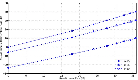
the Reed-Muller decoding of [HCS08] and SIR (this thesis) for N = 1048576 and M = 1024. The SIR is based on a random (20,7) sum-mary codebook. . . 112 4.9 Average recovery-error ratio (SER) versus average

signal-to-noise-ratio (SNR) for different sublinear algorithms. The parameters are N = 220 _and _M _{= 1024 for the Reed-Muller and SIR algorithms,}

and N = 220 _and _M _{= 3780 for the Chaining Pursuit method. The}

sparsity is k = 10. . . 113 5.1 Illustration of a nonuniformly sparse signal . . . 127 5.2 A natural image (left) and the amplitude of its two-dimensional DCT

(12)

5.3 An overlay of satellite images showing the Earth at night . . . 128 5.4 δc as a function of ω=

wK₂

wK1

for γ1 =γ2 = 0.5 . . . 136

5.5 (a) Optimum value of weight ω = wK2

wK1

vs. p2 = p1/5, γ1 =γ2 = 0.5.

(b) Optimum value of weight ω = wK2

wK1

vs. p1

p2, for γ1 = γ2 = 0.5,

p1γ1+p2γ2 = 0.5. . . 136

5.6 Illustration of the improvement in the recovery threshold of Basis Pur-suit for nonuniformly sparse models using the optimal regularization . 140 5.7 A weighted `1-ball, Pw, in R3 (a), and a linear hyperplane Z passing

through a point xin the interior of a one-dimensional face of _Pw (b) . 144

5.8 Empirical recovery percentage of weighed`1 minimization for different

weight values ω, and different number of measurements δ = m_n and

n= 200. Signals have been selected from a nonuniform sparse models. White indicates perfect recovery.. . . 155 5.9 Empirical probability of successful recovery for weighted `1

minimiza-tion with different weights (unitary weight for the first subclass and

ω for the second one) and suboptimal weights in a nonuniform sparse setting. p2 = 0.05, γ1 = γ2 = 0.5, and m = 0.5n = 100. ω∗ in (b) is

the optimum value of ω for each p1 among the values shown in (a). . 156

5.10 Empirical probability of successful recovery for different weights. p2 =

0.1,γ1 =γ2 = 0.5 and m= 0.75n = 150 . . . 156

5.11 Probability of successful recovery (empirical) of nonuniform sparse sig-nals withγ1 = 0.25, γ2 = 0.75, p1γ1+p2γ2 = 0.3 vs. the sparsity of the

second subclassp2. δ = 0.45. . . 157

5.12 Signal-to-recovery-error ratio for weighted`1minimization with weight

ω vs. input SNR for nonuniform sparse signals with γ1 = γ2 = 0.5,

p1 = 0.4, p2 = 0.05 superimposed with Gaussian noise . . . 158

5.13 Average signal-to-recovery error ratio for weighted `1 minimization

with weight ω vs. input SNR for nonuniform sparse signals with

(13)

5.14 Satellite images taken from the New Britain rainforest in Papua Guina at 1989 (left) and 2000 (right). Red boxes identify the subframe used for the experiment, and green boxes identify the regions with higher associated weight in the weighted `1 recovery. Image belongs to the

Royal Society for the Protection of Birds and was taken from an article on deforestation in the Guardian archive [sta]. . . 159 5.15 Functional MRI images of the brain at two different instances

illus-trating the brain activity. Green boxes identify the region with higher associated weight in the weighted `1 recovery. Image is adopted from

https://sites.google.com/site/psychopharmacology2010/student-wiki-for-quiz-9. . . 160 5.16 Average normalized recovery error for `1 and weighted`1 minimization

recovery of the difference between the subframes of (a) a pair of satellite images shown in Figure 5.14, and (b) the pair of brain fMRI images shown in Figure 5.15. Data is averaged over different realizations of measurement matrices for eachδ. . . 160 6.1 Plot of the weak recovery thresholdµW(δ) for `1 minimization,

calcu-lated based on the formulation of [Sto10] . . . 170 6.2 A pictorial example of a sparse signal and its`1 minimization

approx-imation . . . 171 6.3 Comparison of the weak thresholds of `1 minimization with that of

Algorithm 4 computed empirically for Gaussian sparse signals . . . . 173 6.4 Theoretical lower bound on the correct support estimation of `1

min-imization, as a function of the weak threshold exceeding fraction 0.

The plots are based on the theoretical results of Theorem 6.8.2, and are derived for Gaussian, uniform, and two-sided Rayleigh distributions.187 6.5 Empirical recovery percentage for n= 200 and δ = 0.5555 . . . 189 6.6 Empirical overlap between the support set of a k-sparse vector and

the k-support set of the `1 optimum, for n = 200 and δ = 0.5555.

(14)

6.7 Satellite images taken from the New Britain rainforest in Papua Guina at 1989 (left) and 2000 (right). Red boxes identify the subframe used for the experiment, and green boxes identify the regions with higher associated weight in the weighted `1 recovery. Image belongs to the

Royal Society for the Protection of Birds and was taken from an article on deforestation in the Guardian archive [sta]. . . 190 6.8 Functional MRI images of the brain at two different instances

illus-trating the brain activity. Green boxes identify the region with higher associated weight in the weighted `1 recovery. Image is adopted from

https://sites.google.com/site/psychopharmacology2010/student-wiki-for-quiz-9. . . 191 6.9 Average normalized recovery error for`1, and reweighted`1

minimiza-tion recovery of the difference between the subframes of (a) a pair of satellite images shown in Figure 6.7, and (b) the pair of brain fMRI images shown in Figure 6.8. Data is averaged over different realizations of measurement matrices for eachδ. . . 191 7.1 Schematics of a channel coding scheme . . . 198 7.2 Approximate upper bound for the robustness factorC as a function of

error probabilityp for dc= 6 and dv = 3, based on Theorem 7.5.6 . . 218

7.3 BER curves as a function of channel flip probability p, for LP decod-ing and different iterative schemes; random facet guessdecod-ing of [DGW09], mixed integer method of [DYW07], and the suggested iterative reweighted LP of Algorithm 5. The code is a random LDPC(3,4) of lengthn= 1000.226 8.1 Empirical recovery thresholds of Algorithm 6 and NNM for 50_×50

(15)

List of Algorithms

1 —Reverse Expansion Recovery (REVEX) . . . 55

2 —Summarized Index Recovery . . . 102

3 —Mix and Match . . . 104

4 —Two-Step Reweighted `1 minimization. . . 171

5 —Reweighted LP Decoding. . . 220

6 —M-REVEX: Reconstruct a low-rank PSD matrix X from under-determined linear measurements Y =Pd i=1AiXA∗i. . . 243

(16)

Chapter 1

Introduction

Information theory teaches us that if data contains redundancy, it can be reliably compressed without losing the essential information content. Claude Shannon (1916– 2001) quantified this statement by introducing the mathematical notion of informa-tion, and proposing a model for measuring it [Sha48]. In this model, information rate is somewhat equivalent to the measure of uncertainty in random data. Given this mathematical model, it is possible to accurately measure the uncertainty of a data source, or the joint information rate of data generated by various sources. Further-more, using the same mathematical foundation, it is possible to quantify the reliability between the input and output of a communication channel. The former led to the development of source coding, which studies the limits and methods of reliably com-pressing data, and leads to ways for efficiently “storing” information. The latter laid the foundation for the field of channel coding that addresses reliable communication, or more generally “processing” data. In both cases, redundancy in the information content plays a major role, and information theory provides a way of quantifying and exploiting it. In source coding, one attempts to identify or predict the redundancy in the data and eliminate it. In channel coding, the goal is to add redundancy to the data so that the information content can be retrieved despite errors encountered while processing it.

(17)

1.1

Sparsity Is Common

A very common form of redundancy that exists in data extracted from natural events is “sparsity”. The information content of many real-world signals is sparsely dis-tributed, either in the original domain, or when projected via popular transforms. A signal can represent a database, a portfolio, a time-series function, a power spectral density, a probability distribution function, an array of numbers or any other form of

indexed information derived from raw or processed data. The coarse definition of a sparse signal is a vector in which most of the nonzero entries are (almost) zero, and only a few coefficients are nonzero or significant. If the entries of a signal represent the energy content of an object, then a sparse signal has a highly unbalanced energy distribution. Sparse vector representations are conceivable in almost every practi-cal application, from cosine or wavelet transforms of images and video frames, to spectral content of radar signals, to neural records, DNA micro-array read-outs, and fMRI images in genomic and biomedical applications. Further applications arise in sparse covariance matrices in dynamic systems, sparse principle component analysis (PCA) in machine learning, and portfolio representations in financial engineering and economics.

1.2

Sparse Recovery

(18)

of compressed sensing has drawn a lot of recent attention and has evolved into an in-dependent area of signal processing [ric]. Compressed sensing addresses the following

sparse linear inverse problem:

Identify a sparse vector, given a set oflinear combinations of the entries.

In other words, the objective is to identify a sparse vector from a set of linear measure-ments (observations). What makes this theory interesting is that for sparse signals, it is possible to successfully solve the inverse problem even when the number of linear observations is less than the number of unknowns, namely the dimension of the signal. In other words, it is possible to solve an under-determined linear system of equations provided that the unknown signal is sparse.

1.2.1

Mathematical Formulation

Suppose that x _∈ _Rn _{is a vector with at most} _{k << n} _{nonzero coefficients. We}

call such a vector k-sparse. Assume that x is not directly observable, but is rather accessed through a succinct set of linear measurements in the form of:

ym×1 =Am×nxn×1, (1.2.1) where the number of measurements m is smaller than the ambient dimension of x, i.e. m < n. The measurements can be noisy, in which case, we have:

ym×1 =Am×nxn×1+vm×1, (1.2.2) The set of linear equations in (1.2.1) is under-determined (see Figure 1.1). Therefore, there are many vectors x0 that satisfy the above equation. If fact if, x0 is the linear addition of x with an arbitrary vector z in the null space of A (i.e. Az = 0), then

Ax0 = y, and x0 is a solution of (1.2.1). However, it is hoped that the “sparse” solution of (1.2.1) is unique and can be determined. To see this, suppose that x and

(19)

4

Amin Khajehnejad Iterative optimization for compressed sensing and coding

1

Compresses Sensing

Linear inverse problem:

=

m

n

A

x

y

k

A

: measurement matrix, regressors, sketches, encoder

y

: measurements, observations, compression, …

+

noise

compressible

Sparse

[image:19.612.137.519.66.300.2]

(compressible)

Figure 1.1: A pictorial demonstration of an under-determined system of linear equa-tions acting on a sparse (compressible) vector

Ax=Ax0 =y. (1.2.3)

Then, A(x₋x0) = 0. However, the vector x₋x0 has at most 2k nonzero entries. Therefore, to prevent the coexistence of two sparse solutions, it suffices to ensure that no 2k columns of A are linearly dependent. This is not very hard to guarantee if k

is small enough. In fact, a simple dimension counting argument reveals that if the columns ofA are chosen uniformly at random on the unit sphere in_Rm, then as long as k _≤ m/2, this happens with probability 1; Every 2k columns of A are linearly independent and thus every k-sparse solution of (1.2.1) is the onlyk-sparse solution. The same argument holds when the original signal is not sparse per se, but is known to be sparse over some linear “dictionary”. In other words, assume that x

is a vector to be estimated, which is sparse with respect to a linear dictionary (or transformation) Dn×n. In other words, ϕ = Dx is sparse. Assuming that D is an invertible matrix, we can write:

(20)

where Φ _, AD−1_{. The latter is an under-determined system of equations with the}

unknown ϕ being sparse, and therefore has the same structure as (1.2.1). Examples of well-known linear dictionaries include: Fourier, cosine, wavelet, chirplet and Gabor transforms.

A more important question than the uniqueness of a sparse solution is how to recover it? The problem of finding the “the sparsest solution” to (1.2.1) can be written as an optimization program:

min

Ax=ykxk0, (1.2.5)

where the `0 norm of a vector kxk0 is defined as the number of nonzero entries in

x, which is a non-convex function. Therefore, (1.2.5) is a non-convex optimization problem for which no known efficient solvers exist. In fact, an exhaustive search approach can solve this problem as follows: consider every collection of k columns of A, and try to find an inverse solution x assuming that the nonzero entries of x

are restricted to the indices corresponding to the considered set of columns. In other words, try every possible “support set” for the vectorx. Sincem > k, these systems will be over-determined and only the correct support will yield a consistentx0. This

approach takes n_k

operations and, unlessk =O(1), is exponentially complex. One possible way to overcome the computational intensity is try to approximate (1.2.5) with a convex optimization. The closest convex relaxation to the `0 norm is

the `1 norm defined as the sum of absolute values of the entries of x. The resulting

optimization becomes:

min

Ax=ykxk1. (1.2.6)

In fact, (1.2.6) is a linear program, and many efficient methods exist that can solve it in time polynomial in n (_O(n3) to be precise).

(21)

the sparse recovery problems (1.2.1) and (1.2.5), including the convex optimization of (1.2.6). In this context, (1.2.6) is commonly known as`1 minimization, `1 regression,

or Basis Pursuit, and has been extensively studied. We will soon return to discuss this in more details.

1.2.2

Interpretations

The linear inverse problem described in (1.2.1) can be interpreted in various ways depending on the context and physical application. We consider the following different outlooks.

Sub-Nyquist Sampling

Compressed sensing can be regarded as a method of sampling signals at sub-Nyquist rates, or equivalently a technique for jointly sampling and compressing real time analog data. The fundamental Shannon-Nyquist sampling theorem states that a continuous-time band-limited signal can be sampled at discrete points at a frequency rate equal to twice the bandwidth of the signal, without compromising the information content [Mar06]. This statement is very helpful in designing analog-to-digital systems and determines the bottleneck in storing and processing continuous real-time signals. Compressed sensing theory provides means of achieving lower sampling rates than the Nyquist rate. Assume the vector ϕ = (ϕ1,· · · , ϕn)T represents samples of a a

band-limited function f(t) taken at the fundamental Nyquist rate:

ϕi =f(i/T), 1≤i≤n, (1.2.7)

where T = 1/(2B) is the sampling period, and B is the bandwidth of f(t). The band-limited assumption on f(t) assures that the frequency content of f(_·) has a lot of vacancy, or equivalently that the vectorx=Fϕ is approximately sparse, whereF

(22)

a_i

t = iT



A = [a₁, a₂, … , a_n]

f(t) f(t)

t 2πB 2πB ω

F(ω)

Figure 1.2: Schematics of a sub-Nyquist sampling system

y=AFφ=Ax, (1.2.8)

where AF is a matrix appropriated for compressed sensing with m < n rows. The resulting sampling rate is thus m_n_T1. When applied to real-time signals or streams of data, the matrix A acts as a correlation operator, and is therefore referred to as the

correlation matrix orsketches (see Figure 1.2). For more information on this subject please refer to [ME11].

Estimation Under Ill-Conditioned Observations.

Another interpretation of the linear inverse problem (1.2.2) is linear regression under an under-determined set of observations. In the linear regression model, x

(statisticians prefer β) refers to a set of parameters of a regression model to be esti-mated. The entries of A are called regressors. Different rows of A are independent realizations of independent variables, and y is the regressand vector.

The objective of regression models is usually to minimize the estimation risk. The (co)statistics of the parameters x and the error terms v should be known, and depending on the risk criteria chosen, different estimators can be selected. Least square and maximum likelihood solutions are archetypes of estimation criteria. When

(23)

other conditions such as sparsity must be assumed for the parameters. Sparse linear regression models can be studied in the context of Bayesian compressed sensing [duk, JXC08].

Source Coding Scheme

Compressed sensing can also be regarded as an analog compression scheme for peeling off the redundancy of a sparse generating source. In this case, the matrix A

is in fact anencoding matrix, and reconstruction is adecoding algorithm. Information theoretic bounds can be found that relate the compression rate to the information rate of sparse sources, as well as trade-offs between the compression rate and quantization error [FRG07] (rate distortion theory for compressed sensing).

Data Privacy

Suppose that x represents a private database, not directly accessible to outside users. The database can however be observed through random queries in the form of linear projections corrupted by noise, as y = Ax+v. Understanding the limits of sparse recovery in such statistical setting helps protect private data, say by adding the right amount of noise. This model of privacy and its connection to compressed sensing has been studied in [DMT07].

1.2.3

History

Deconvolution of sparse signals using `1 regularized estimators dates back to the

1960s [Log65]. Starting in the 1970s, the use of such techniques became popular in determining marine surface structures from the reflection of acoustic pulses [TBM79]. Seismological traces are the convolution of a source wavelet (acoustic wave) with the impulse response of the marine surface which is often a sparse train of spikes [CB83]. Therefore sparse-promoting linear solvers such as `1 norm regularized least square

techniques were used to extract surface patterns. In the 1990s and with the advent of powerful computerized solvers for linear programs, `1 regularized regressions were

(24)

minimization in the context of signal representation under alternative dictionaries, and suggested the Basis Pursuit (BP) method for atomic decomposition of signals in overcomplete dictionaries [CDS01]. Donoho’s proposed scheme was in contrast to the rising Matching Pursuit (MP) algorithm proposed slightly earlier by Mallat and Zhang [MZ93]. The MP method was introduced as a way of denoising signals that are sparsely representable over redundant dictionaries. MP is a greedy algorithm that iteratively selects a basis function that matches best (i.e. has the highest corre-lation) with the signal projection. Tibshirani proposed the least absolute shrinkage and selection operator (LASSO) in 1996, an`1-norm-bounded constraint least-square

minimization, and argued that LASSO is advantageous to most regression techniques in sparse model fitting [Tib96]. LASSO was studied in the context of Bayesian es-timation, specifically for model fitting in medical applications [Tib97]. However, to this point, most of the results remained mainly empirical.

In the early 2000s an explosion of analytical results on sparse recovery techniques occurred. Donoho et al. first proved that for measurement matrices (or overcomplete dictionaries as preferred by some) with a sufficiently large mutual coherence, Basis Pursuit has a stable recovery in the presence of noise, provided that the unknown sig-nal is sufficiently sparse [DET06]. Following that, in a series of breakthrough papers, Cand`es, Romberg, and Tao proved that `1 minimization allows exact reconstruction

(25)

that pairwise distances between sparse vectors is approximately preserved (thus the word isometry) when projected by A. Cand`es and Tao further proved that random matrices with Gaussian entries satisfy RIP, and thus recovery of sparse signals and stable recovery of approximately sparse signals with an order-wise optimal number of measurements is possible. Soon after that, Donoho and Tanner proved similar universality results for BP under random projections and provided stronger guaran-tees than the previous results. Donoho et al. defined the notion of neighborliness

for high-dimensional polytopes. k-neighborliness for a polytope implies that every subset of k vertices form a k ₋1 dimensional face, and are thus neighbors in that sense. The object with the highest order of neighborliness in_Rn _{is the}_n_-dimensional

simplex. Donoho et al. proved that successful sparse reconstruction of k-sparse vectors using BP is equivalent to the k-neighborliness of the n-dimensional simplex projected by A [Don06b, DT05a, DT05b]. Under the assumption of asymptotically large vector size n, and proportional system dimensions, i.e. m = Θ(n), k = Θ(n), it is possible to analyze the neighborliness property for random projections such as Gaussian measurements. The analysis requires advanced high-dimensional convex geometry techniques. Under such circumstances, Donoho et al. derived tight bounds known as recovery thresholds that accurately predict the success of `1 minimization

for large-dimensional inverse systems. The characterization of the recovery thresh-olds presented by Donoho et al. is very involved, and does not allow for further exploring these bounds. Later works done by Xu et al. and Stojnic et al. came with easier characterizations and extensions of the recovery thresholds of `1

mini-mization [SXH08, XT10b, Sto10, Sto]. Specifically, [SXH08] provided an equivalent condition for the neighborliness property, which is expressed in terms of the null space of the measurement matrix. These null space properties are easier to analyze and re-sult in a so-called “Grassmann manifold” framework for the study of the properties of `1 minimization. Using this framework, [XT10b] provided a tight analysis of the

(26)

under the presence of noise and for approximately sparse signals. The more recent work of Stojnic et al. is based on a technique called “escape through the mesh” and results in much simpler and more explicit calculations for the thresholds of Basis Pursuit under than the Grassmann manifold approach.

Interest in the theory of sparse recovery sharply increased after the fundamental results of Donoho and Cand`es. Alongside the convex optimization methods, greedy algorithms were also revisited in the hope of more rigorous analysis. The Match-ing Pursuit technique was first refined to a more stable Orthogonal MathMatch-ing Pursuit (OMP) algorithm [PRK93, DMA97] without presenting significance analytical guar-antees. OMP was studied later by various researchers including Chen et al. and Tropp et al. in the 2000s [CH06, Tro04, TGS06, TG07]. Specifically, it was shown in [TG07] that under the assumption that A is random Gaussian, m = _O(klogn) measurements are sufficient to guarantee successful recovery of sparsek-sparse signals with high probability, a bound which is order-wise equivalent to that of BP. Donoho et al. introduced a more advanced version of OMP called Stagewise Orthogonal Matching Pursuit (StOMP), and showed empirically that their proposed method has superior performance to Basis Pursuit in the asymptotical proportional regime for extremely under-determined systems (m_n << 1) [DTDS06]. Needell and Tropp pro-posed CoSaMP, a method that has a faster running time than OMP and guaranteed stability to noise [NT08].

Many more varieties of the described algorithms have been proposed over the past few years, and many alternative techniques have been developed. Today, sparse re-construction techniques are not limited to convex relaxation or greedy approaches, and contain a vast number of alternative iterative, combinatorial, and algebraic tech-niques. We will mention many such techniques in the later chapters of this thesis.

1.2.4

A Few Fundamental Questions

(27)

What is a good reconstruction algorithm?

A good algorithm should be efficient, resilient to noise, and easy to implement. Fur-thermore, the exact definitions of these criteria depends on the particular application to which sparse estimation is mapped.

What are good measurement matrices A?

In addition to identifying matrices that make the reconstruction a feasible task, it is important to design structures that are amenable to certain recovery algorithms and vice versa.

What happens in the presence of noise?

In the presence of noisev, we are interested in the “robustness” of recovery algorithms. Assume that ˆxis an approximation to xprovided by a reconstruction algorithm. We say that the recovery algorithm is robust if for some norm functions f, g, and a constant cwe can guarantee the following:

f(x₋xˆ)_≤c_·g(v). (1.2.9) .

What is the minimum number of measurements required for successful sparse estimation?

This question is very important, as its answer determines the performance limits of sparse recovery algorithms.

What is the tradeoff between performance and noise/quantization error level in sparse recovery?

(28)

How can an algorithm/matrix be tailored to a particular application?

As we will see, some measurement matrices and recovery algorithms are suitable for particular applications due to the inherent nature of the application, or for simplicity of implementation. This question has practical advantages too.

Is there an efficient method for assessing the goodness of an arbitrary measurement matrix A?

It is very important to have deterministic guarantees for practical applications. If A

is a large measurement matrix, is it possible to determine (in a reasonable time) how good of an encoding matrix it is? In other words, is there a performance metric for a matrix with regards to sparse compression/decompression that can be verified in efficient time?

These questions (or criteria based on these questions) have served as the road map for research on sparse linear inverse problems. Below we briefly discuss the existing methodologies and guarantees in response to the above questions.

1.2.5

Existing Methodology

Random matrix ensembles are commonly used as the measurement matrix in the study of sparse recovery problems. The original results of compressed sensing were based on matrices with i.i.d Gaussian matrices [CT06a, CT05, Don06b] but were soon extended to other distributions such as Bernoulli or random _±1 entries [BDDW08, DT10], and generally to all sub-Gaussian distributions [MPJ09, CR11]. Furthermore, random partial sub-dictionaries of most well-known dictionaries form relatively good measurement matrices. For instance, random selection of m rows from the n_× n

(29)

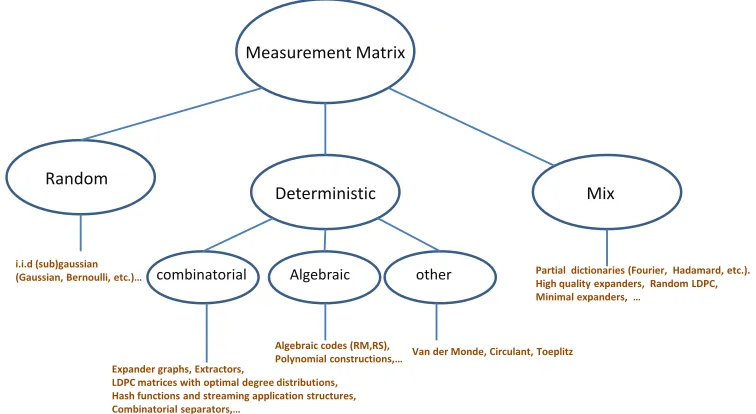
and high dimensional convex geometry techniques. However, a number of combinato-rial and deterministic structures have also been introduced, due to practical benefits such as lower cost of encoding, ease of implementation, and better reconstruction algorithms. The most common classes of such matrices are sparse binary matri-ces, such as expander graphs [Ind08, XH07b], measurement matrices based on LDPC error-correcting codes, Van der Monde matrices [DeV06], circulant and Toeplitz struc-tures [Rau], measurement matrices based on algebraic error-correcting codes such as Reed-Solomon, Reed-Muller, and p-ary codes [HCS08, PH08, AM11, AMM12], ma-trices based on hash functions and sketches used for streaming applications [CM04, CM05, CM06], and others (see e.g. [GSTV06, DMP11]). The diagram in Figure 1.3 summarizes these different categories of existing measurement matrices.

1

Methodology

Introduction

Measurement Matrix

Random

Deterministic Mix

combinatorial Algebraic other

Expander graphs, Extractors,

LDPC matrices with optimal degree distributions, Hash functions and streaming application structures, Combinatorial separators,…

Algebraic codes (RM,RS), Polynomial constructions,…

Partial dictionaries (Fourier, Hadamard, etc.). High quality expanders, Random LDPC, Minimal expanders, …

Van der Monde, Circulant, Toeplitz i.i.d (sub)gaussian

[image:29.612.137.515.338.545.2]

(Gaussian, Bernoulli, etc.)…

Figure 1.3: Summary of existing categories of measurement matrices for compressed sensing with examples

(30)

on convex optimization. BP is the `1 minimization program described in (1.2.6).

BPDN [CDS01] is a quadratic programming which is essentially a regularized La-grangian of the constrained `1 minimization:

BPDN min 1₂_kAx₋y_k2

2+λkxk1. (1.2.10)

Other similar estimators have been used based on alternative forms of regularization which are common in statistical estimation, such as the LASSO [Tib96] and Dantzig selector [CT07]:

LASSO min 1₂_kAx₋y_k2₂

subject to_kx_k1 ≤t. (1.2.11)

DS min_kx_k1

subject to_kAt(Ax₋y)_k∞. (1.2.12)

Greedy algorithms are mostly based on iterative approximations to a sparse solu-tion, such as the Matching Pursuit method and its variations (OMP [TG07, CH06, Tro04, TGS06], StOPM [DTDS06], CoSaMP [NT08, NTV08], etc.), iterative least square techniques [DDFG10, CY08], and iterative thresholding methods [FR08, BD08]. These methods are generally inferior to their corresponding convex program as they require more careful regularization, but are easier to implement.

(31)

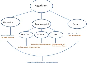
graphs, such as the bit flipping decoding algorithm [XH07b], expander Matching Pur-suit (EMP) [IR08], sparse Matching PurPur-suit (SMP) [BIR08], and sequential Sparse Matching Pursuit (SSMP) [BI09], list-decoding algorithms and other reconstruction methods for constructions based on algebraic error-correcting codes [HCS08, HSC09, PH08], algorithms based on data streaming applications [CM05], message-passing decoding [CSW10, LMP08], Chaining Pursuit [GSTV06], and many more. The di-agram in Figure 1.4 summarizes these different categories of existing reconstruction algorithm.

1

Methodology

Introduction

Algorithms

Geometric

Combinatorial Greedy

Expanders Algebraic other

Bit flipping, EMP, SMP, SSMP, REVEX

List decoding, Chirp reconstruction

MP and variations: OMP, StOMP, CoSaMP

Message passing , CP, Data streaming alg.’s, … Convex optimization:

BP, BPDN, LASSO, DS

[image:31.612.141.510.267.533.2]

Iterative thresholding, Iterative convex optimization

Figure 1.4: Summary of existing categories of algorithms for compressed sensing with examples

1.2.6

Applications

(32)

Image and Video Processing

Many forms of images are approximately sparse over some well-known dictionary. For example, natural images over the discrete cosine transform (DCT) domain are known to be concentrated mostly on lower frequencies. Astronomical images are often sparse in their regular spatial domain. Consecutive frames of a high-speed video have sparse residual. In light of this, image acquisition systems based on compressed sensing have two possible mechanisms. An original high-resolution image can be compressed using a linear encoding matrix. Alternatively, an input image can be directly measured and stored in the form of linear projections. The former is a compression scheme which is helpful in maintaining large databases. The latter is in particular useful in biomedical imaging, such as magnetic resonance imaging (MRI) [LDP07, LDSP08, KNN09], where obtaining higher resolution images requires patients to be exposed to stimulating signals (e.g. electromagnetic waves in an MRI scanner) for long periods of time. Linear combinations of image components (over some dictionary, such as wavelet) can instead be obtained by simultaneously combining different components of the stimulating signal. A reconstruction algorithm can then be used to recover the desired information. A similar application of this approach is in image or video cameras that record linear combinations of pixel intensities or consecutive frames, instead of a super-high-resolution pixel array [VRR11]. These ideas have led to the development of prototypes for imaging devices that function based on compressive sampling technologies, such as the single-pixel camera [DDT+_08].

Radar

(33)

receiving continuous time pulses, but need to digitize data for processing. Sparse time-frequency spectrums can be sensed at higher rates using compressive sampling. Instead of sampling continuous time signals and digitizing the samples, we can obtain linear projections of the input stream using high-speed correlation circuits, and then digitize the projections [HS09]. Also, please refer to [CV08] for an alternative use of sparse recovery in MIMO radar detection.

Beyond radar applications, achieving higher A/D rates is extremely motivated, and numerous attempts at implementing analog-to-information compressed-sensing-based systems have been reported over the past few years [LKD+07].

DNA Micro-Array

Micro-arrays are large sets of parallel microscopic DNA probes that can detect the expression levels and consequently identify the absence or presence of different genes inside a DNA genome solution. DNAs and RNAs can bind to the probes by a process called hybridization. Conventional DNA micro-arrays work based on the principle that every probe detects at most one target DNA sequence, and thus require a large number of genomic probes. In addition, cross-hybridization is a common phenomenon which degrades the performance of the sensor array. In contrast, a new micro-array technology which is based on compressed sensing has been developed where multiple DNA sequences can bind to each probe. The probes read-outs are thus roughly equal to linear combinations of gene expression levels. Sparse reconstruction algorithms are invoked to estimate the existing DNA genes and their expression levels [PVMH08, DMSB08, MBSR07, ES05, VPMH07].

Networks

(34)

ad-hoc networks [ZLG], and clique identification in social networks [JYG09].

Communications

Compressive sampling has led to novel mechanisms for sparse channel estimation, spectrum sensing, interference alignment, user detection, and design of communi-cation protocols in wireless MIMO and ad-hoc networks over the past decade (see, e.g. [BHRN08, BHSN10, TH08]). For a comprehensive study, we refer the interested reader to the references provided in [ric].

More

Applications of sparse reconstruction techniques are not limited to the above exam-ples. There are many more applications where a sparse linear inverse model accurately fits. This includes almost all areas of signal processing from financial engineering to astronomy. However, it is important to note that the requirements, methodology, and existing guarantees can be very different from one application to another. We will discuss this issue in more detail in future chapters.

1.3

Beyond Compressive Sampling

In many cases, there are other forms of common non-linear transforms that result in sparse (or compressible) representations of certain classes of signals. For example, if the unknown signal is a matrix Xn×n _{of rank} _{k << n}_{, then the singular value}

decomposition (SVD) of X results in a sparse set of singular values consisting of only

(35)

highly motivated under the terms “rank minimization” and “matrix completion”. Re-construction of rank-deficient matrices from ill-posed lower projections or completion of such matrices from partially known entries is motivated by problems in covariance estimation, dynamic systems, quantum computation, and collaborative filtering. A great example is the well-known Netflix problem, the objective of which is to predict ratings of different movies by a large number of users. The results of such predic-tion would help Netflix provide targeted recommendapredic-tions to its users. The table of users/movie ratings is a two-dimensional matrix that needs to be estimated in this case. A valid assumption often made is that by nature, such matrices are approxi-mately low rank as many users tend to have similar or highly correlated interests. In addition, only a fraction of the target matrix is often available in the form of random entries, and the rest is to be estimated. The problem is therefore that of matrix rank minimization. Similar models show up in other forms of recommendation systems and search engines, such as the Google PageRank problem [AT05].

Matrix rank minimization and low-rank matrix completion have been the center of attention by many in the past few years. Fazel et al. proposed using a convex heuristic known as nuclear norm minimization (NNM) to estimate low-rank matrices. Nuclear norm is a convex relaxation to the rank function of a matrix and thus a low-rank promoting regularizer. This approach is very similar to the use of`1 minimization in

compressed sensing. Rigorous analysis of the NNM method has been done in [RFP10, RXH08, OH, CR09, CT10]. However, despite significant efforts, little progress has been made when compared to compressed sensing. For example scant work exists on faster reconstruction algorithms or alternative forms of projections. Therefore, matrix rank minimization is currently a very open and motivated field of research.

1.4

Contributions of This Thesis

(36)

restricted to specific contexts and applications. In this dissertation, we have tried to understand the boundaries of existing knowledge and methodology on sparse recovery techniques, and extend them in various ways. Below is a summary of the contributions of the current thesis and the descriptions of how they fit into the state-of-the-art literature.

1.4.1

Compressed Sensing

The seminal results of Cand`es et al. and Donoho et al. [CT05, Don06a] established that a class of convex optimization methods can solve the sparse linear inverse prob-lem much more efficiently than exhaustive search. As discussed, these methods are known as Basis Pursuit or`1-regression techniques, and require an order-wise optimal

number of measurements m = _O(klog(n/k)) to succeed. Basis Pursuit algorithms are popular because they have universal guarantees and computable phase transition thresholds, and have a polynomial complexity _O(n3_{) that allow them to be}

(37)

methods are tailored to specific measurement matrices. Designing matrix structures that are amenable to existing or new methods of sparse reconstruction is therefore as important as algorithm development. In light of these issues, our contributions fall in the the following categories:

Deterministic Measurement Matrices

Although the performance of random and dense measurement matrices are easier to analyze, they pose several practical limitations, including extensive memory require-ments, high recovery complexity, and lack of deterministic guarantees. One of our objectives is developing deterministic and/or sparse matrix constructions for sparse recovery, either for the existing reconstruction algorithms (such as Basis Pursuit), or in conjunction with novel estimation methods. In either case, providing theoret-ical guarantees for the proposed construction/reconstruction schemes is imperative. Three main categories of novel deterministic structures discussed in this thesis are the following:

• Minimal expander structures. Expander graphs are combinatorial objects with unique features that make them useful in various applications. Despite having small vertex degree, i.e. being sparse, the overall connectivity of expander graphs is high, and thus leads to fast mixing times, making them good candidates for Monte Carlo methods and as error-correcting codes. Expander graphs are characterized by an expansion coefficient 0 < < 11. Larger corresponds to better connectivity and smaller mixing times.

A recent research trend has proposed using bipartite expander graphs as com-pressed sensing measurement matrices, leading to a number of combinatorial al-gorithms and methods to analyze Basis Pursuit for sparse constructions [XH07b, BGI+_{08]. Results in the literature prior to the contributions of this thesis only}

consid-ered high-quality expander graphs with expansion coefficients_≥3/4. It is generally

(38)

harder to construct expanders with higher expansion coefficients, and consequently the required oversampling factorsm/kfor successful recovery of sparse signals become extremely large. For example, when a compression ratio m/n = 0.5 is considered, the best existing results for high-quality expanders only guarantee2 _{that sparsity}

frac-tions k/n _≈ 10−6 _{can be reconstructed efficiently. This means there should only be}

one nonzero coefficient in a million! In contrast, we introduce a class of minimal expanders in Chapter 2 with much smaller values, that can be deterministically constructed. We have analyzed the proposed constructions in the realm of the Basis Pursuit algorithm [KXDH10]. The resulting guaranteed sparsity fractions can be as high as k/n _≈ 10−2_{, filling the gap between the performance of dense and sparse}

measurement matrices for compressive sensing. Chapter 2 of this thesis is devoted to this subject.

• Binary structures based on graphs with logarithmic girth. Using results from channel coding, we have developed novel constructions for the measurement matrix A. “Good” channel coding parity check matrices form “good” measurement matrices for compressed sensing. Using this idea, we have studied several construc-tions of LDPC codes in the context of compressed sensing that result in even tighter provable thresholds than minimal expanders. We show that the structure of the Tan-ner graph of a code and some of its fundamental properties, such as the minimum cycle length (girth) can be used to assess the goodness of a given binary matrix with respect to Basis Pursuit algorithms. The importance of this criterion is that it can be checked in polynomial time. Specifically, we show that LDPC codes with Ω(log(n)) girth offer very tight thresholds for the number of measurements for a robust `1/`1

approximation noise [KTDH11]. Our bounds are the tightest existing guarantees us-ing sparse measurement matrices. These ideas are discussed in detail in Chapter 3 of this thesis.

(39)

• Summary-based structures for very fast and sub-linear compressed sens-ing. There are many instance of sparse recovery problems where the signal dimension is extremely large (say n = 106_–1012_{), and the number of significant nonzero entries}

in the signal is in the range of 100–1000. Important examples where this setup arises are neighbor discovery in ad-hoc sensor networks and efficient multi-user RF-ID. In these cases, conventional recovery methods with recovery times polynomial innfail in practice, as n is very large. Therefore, algorithms with “sub-linear” complexity have to be developed, where the complexity is logarithmic in n, i.e. _O(poly(log(n))), and polynomial in k. We have developed a new class of measurement structures with the motivation of designing algorithms that have a sub-linear complexity in the system dimension. These constructions will be presented in Chapter 4. The matrices that we propose are highly structured and facilitate summarized searches over the span of the unknown vector. Using ideas from combinatorial separators and hash functions, we developed matrices based on binary labeling and sub-labeling of the state space. In addition to the obvious time/memory advantages that result from the fast recon-struction algorithms we propose for these structures, the underlying conrecon-structions are greatly motivated by a variety of statistical inference problems such as popular political ranking, market basket analysis, revenue maximization, graphical models, and so on. In many cases, the regressors of the inference problem are in the form of a matrix A similar to summary based structures (see e.g. [KKH11, JS08, JYG09]). Chapter 4 is dedicated to these concepts.

Recovery Algorithms

(40)

transition threshold, which is explicitly computable. However, an important open problem is whether there exist other polynomial time algorithms that have superior thresholds to those of Basis Pursuit. This problem is addressed in this dissertation. A solution is provided that holds for most cases, with the exception of a restricted class of random signals where the distribution of the nonzero entries and all its finite derivatives vanish at the origin. For example, binary (0,1) and ternary (0,_±1) sparse vectors are of this type.

Below is a summary of sparse recovery algorithms that will be introduced and analyzed in this thesis:

• Two-step reweighted Basis Pursuit. In Chapter 6, we introduce a two-step linear programming algorithm and prove that for many classes of random sparse sig-nals, the proposed method has better phase transition thresholds than Basis Pursuit. To our knowledge this is the only result of this kind. The proposed algorithm is based on coarsely approximating the support set of a sparse signal with the help of Basis Pursuit, and separating the entries based on whether we “believe” they are zero or nonzero. Then, a second linear program is performed, in which the entries that are believed to be zero are penalized with a larger weight. The practical improvement of the proposed scheme is significant. For instance, for a compression ratio m/n= 0.5, the recoverable sparsity ratio k/n can be improved by 20%.

• Reverse expansion linear inversion (REVEX) algorithm for minimal ex-panders. We propose this algorithm in Chapter 2. In particular, this is an algorithm designed for the minimal expander constructions which will also be explained in Chap-ter 2. The method has _O(k2n) complexity, which makes it significantly faster than Basis Pursuit (_O(n3_{)) for the corresponding expander codes, and has a theoretically}

equivalent performance.

(41)

which will be explained in Chapter 4. The routine is extraordinarily fast and can han-dle recovery of sparse sample points in extremely large dimensions. Theoretically, the decoding complexity is _O(kmlog(m)) and the required number of measurements is almost optimal m=_O(klog(n) log log(n)). The advantages are not limited to a the-oretical level; the method can be of great practical value. For instance, preliminary simulations reveal that a k = 100 sparse vector of length n = 1012 can be recon-structed usingm _≈5000 measurements within less than a minute on normal desktop computers. These figures are linearly scalable to higher dimensions, and stand far above the state-of-the-art efficient sparse recovery performances. In addition, the noise tolerance of the SIR method is competitive with the best existing methods. Such a combination of strong theoretical guarantees and practical evidence make this framework an ideal candidate for many real-world high-dimensional applications, potentially extending to hardware-level implementation.

1.4.2

Rank Minimization

(42)

operators have two key properties: 1) They have low density, which means that the projection of rank 1 matrices have at most rank d = _O(1), and 2) despite having low density, the operators expand the rank of low-rank inputs, and as such are called “rank expanders”. We propose a combinatorial algorithm that allows for the recon-struction of sufficiently low rank matrices using the proposed rank-expanders. The algorithm resembles the REVEX method developed earlier for minimal expanders in compressed sensing, and in a similar way is significantly faster than geometric meth-ods based on semi-definite programming. Additionally, rank-expanders appear in a number of applications, such as system identification and quantum computing, unlike generic random Gaussian operators, further motivating their use.

1.4.3

LDPC Codes and Improved Channel Coding

(43)

to systematic improvements in a variety of important inference problems.

1.5

Organization

The content of this paper is presented in three main parts. In the first part which contains Chapters 2–4, we discuss new combinatorial structures for the design of mea-surement matrixAin compressed sensing. We study these constructions in detail and evaluate the performance of various reconstruction algorithms based on these designs. An overview of the use of sparse matrices for compressed sensing is given in Chapter 2, and minimal expanders are introduced. In Chapter 3, we study connections be-tween channel coding and compressed sensing, and prove certain performance results for bipartite graphs with logarithmic girth. In Chapter 4, sub-linear time algorithms are motivated and discussed, and summary-based structures are introduced which lend themselves to a very fast and practical reconstruction algorithm.

Part II has a relatively different theme, and is mostly focused on the Basis Pursuit algorithm and random Gaussian measurements for sparse recovery. We study ways to improve the theoretical and practical thresholds of the Basis Pursuit algorithms. These thresholds identify the asymptotic performance of an`1minimization algorithm

for the case of “proportional” system dimensions, i.e. k,m, and n are proportional to each other. In Chapter 5, we show that if prior information is available about the unknown signal in the form of non-uniform sparsity, then weighted `1 algorithms

have higher thresholds than regular Basis Pursuit. In Chapter 6, we introduce and study a two-step reweighted `1 minimization algorithm with many of the technical

tools borrowed from Chapter 5.

Finally, in Part III we generalize some of the results of the previous chapters to low-rank matrix estimation (Chapter 7) and channel coding (Chapter 8).

(44)

and discussions. Simulation results (if any) are presented at the end. For simplicity of reading, we have pushed long proofs to an appendix section at the end of each chapter. A table of important notations is also included before the introduction in each chapter.

1.6

Short Note on Notations

(45)

Part I

Combinatorial Structures for

Sparse Recovery

(46)

Chapter 2

Sparse Minimal Expanders

A measurement matrix

n signal size

m number of measurements

k sparsity of the signal G bipartite graph Γ(S) set of neighbors of S

2.1

Introduction

In this chapter, we focus on the design of sparse (i.e. low density) measurement matrices for compressed sensing. The-low density assumption for the matrices used is crucial for numerous reasons. In several applications, the cost of each measure-ment increases with the number of coordinates of the unknown vector x involved. For instance, in the design of DNA micro-arrays using the CS technology in which the pattern of micro-arrays translates directly to a suitable measurement matrix, every nonzero entry of the matrix represents a probe [PVMH08, DSMB09]. As a result, the overall cost of the micro-array panel is directly ruled by the density of the corresponding matrix. There are several other applications where only a sparse matrix assumption is close to a reasonable approximation of the underlying sketch-ing process (see for example the motivation given in [GI10]). Sparse measurement

(47)

matrices have also made possible the design of faster decoding algorithms (e.g., [IR08, BIR08, XH07b, Tro04, XH07a, JXHC09]), apart from the general linear pro-gramming types of decoder [CRT06b, GLR08] originally proposed for dense matrices. Unlike dense and random constructions (such as i.i.d. Gaussian matrices), where reasonably sharp bounds on the thresholds which guarantee linear programming to recover sparse signals have been obtained [DT05a], such sharp bounds do not exist for sparse measurements. Finding such sharp bounds for the special case where the

k-sparse vector is nonnegative is the main focus of the current chapter. Although the nonnegativity constraint is primarily considered for ease of analysis, it represents a large class of practical interests. Signals arising in many problems are naturally nonnegative. Examples of positive real-world signals are natural or biomedical images, DNA micro-array data, network monitoring data, information collected based on hidden Markov models, and many more examples in which the actual data is of nonnegative nature. Compressed sensing for nonnegative signals has also been studied separately in various previous work [DT05b, BEZ08], but with different approaches.

In the remainder of this chapter, we carefully examine the connection between linear programming recovery and the fundamental properties of the measurement matrix, in light of the fact that the considered matrices are sparse.

2.2

Related Work

For a given measurement matrix, the success of linear programming recovery is often certified by the restricted isometry property (RIP) of the matrix [CT05]. For random dense matrices, these conditions have been studied to a great extent in the past few years. For sparse matrices, however, there were only a handful of promising results at the time when our very first results on this subject were published. Specifically, Berinde et al. [BGI+_{08] showed that the adjacency matrices of suitable unbalanced}

(48)

definition of RIP. However, it turns out that RIP conditions are only sufficient con-ditions for the success of linear programming decoding, and often fail to characterize all the good measurement matrices. A complete characterization of good measure-ment matrices is given in terms of their null spaces [SXH08, FN03, LN06, Zha05]. A necessary and sufficient condition for the success of `1 minimization is therefore

called the “null space property”1. Donoho et al. [Don06b] were the first to prove the validity of this condition with high probability for random i.i.d. Gaussian matrices, and were able to compute fairly tight thresholds regarding when linear-programming-based compressed sensing works [DT05a]. The first analysis of the null space for sparse matrices has been done by Berinde et al. [BI08], where in particular they con-sider measurement matrices that are adjacency matrices of expander graphs. It was shown that every (2k,) expander graph2 with_≤ 1₆ satisfies the null space property, and therefore every k-sparse vector can be recovered from the corresponding linear measurements. The recovery thresholds given by this result, namely the relationship between the sparsity-to-dimension ratio _nk, and the aspect ratio of the measurement matrix m_n for which reconstruction is successful, are governed by the extents at which such suitable expander graphs exist. Expander graphs have either random or ex-plicit construction (see, for example [GLW08] for exex-plicit constructions of expander graphs). In either case, the resulting thresholds of [BI08] are very small (e.g., on the order of 10−5 _for m

n = 0.5), due to the high expansion requirement, i.e., ≤ 1/6. In

contrast, our analysis led to the design of sparse measurement matrices that obtained recovery thresholds around two to three orders of magnitude higher than the bounds of Berinde et al. (e.g., around 0.01 for m_n = 0.5), which, however, holds only for non-negative signals. The null space characterization and its use in compressed sensing has also been studied in [BEZ08], from a quite different perspective. In that paper, the authors show that a so called “coherence” measure on the measurement matrix

(49)

is related to the null space property. Unfortunately, when applied to sparse matrices, this result does not yield very sharp bounds for the recovery threshold either.

Finally, there exist other related works in the literature that address the problem of sparse signal recovery in the case of sparse matrices, but for different recovery methods. The work of Wang et al. [WWR10] attempts to provide general information theoretic bounds for the feasibility of successful recovery, even if it requires brute force endeavor. The reference [ZP] provides a theoretical analysis (based on the density evolution technique) for a message-passing algorithm for recovering sparse signals measured by sparse measurement matrices. Another example is [LMP08], which considers the same problem, but for nonnegative signals. A shortcoming of the density evolution technique is that it can only determine asymptotic (infinite blocklength) results, and relies on an asymptotic limit exchange. Furthermore, it should be clear that, unlike these papers, we focus only on `1 minimization recovery.

A further distinction of our analysis is the provision of a strong bound for sparse recovery, namely the bound for all nonnegative signals, which was not provided in [LMP08]. For further readings on compressive sampling techniques and analysis using sparse matrices, we refer the interested reader to the survey article of [GI10], which overviews recent results, including our own work presented here.

2.3

Contributions

We introduce sparse measurement matrices that result from adding perturbations to the adjacency matrices of expander graphs with a small critical expansion coefficient, hereby referred to as minimal expanders. We show that when`1 minimization is used

(50)

theoretical upper bounds for the so-called “weak” and “strong” recovery thresholds when`1 minimization is used. These bounds are very close (order-wise) to the bounds

of Gaussian matrices for the nonnegative case (Section 2.7 and Figures 2.3 and 2.4). Furthermore, by carefully examining `1 minimization for sparse matrices, we deduce

certain uniqueness results for the nonnegative solution of the linear equation when constant column sum matrices are used (see Section 2.5.1). We exploit this fact later to find faster alternatives to`1 minimization. In particular we present a novel recovery

algorithm that directly leverages the minimal expansion property, and we prove that it is both optimal and robust to noise (Section 2.8).

One critical innovation of our work is that for expander graphs in the context of compressed sensing, we require a much smaller expansion coefficient in order to be effective. Throughout the literature, several sparse matrix constructions rely on adja-cency matrices of expander graphs [BGI+_{08, BI08, XH07b, JXHC09, Ind08]. In these}

works, the technical arguments require very large expansion coefficients, in particular, 1₋ _≥3/4, in order to guarantee a large number of unique neighbors [SS96] to the expanding sets. Our analysis is the first