SOLVING ECONOMIC DISPATCH PROBLEM USING PARTICLE SWARM OPTIMIZATION BY AN EVOLUTIONARY TECHNIQUE FOR INITIALIZING PARTICLES

526

SOLVING ECONOMIC DISPATCH PROBLEM USING

PARTICLE SWARM OPTIMIZATION BY AN

EVOLUTIONARY TECHNIQUE FOR INITIALIZING

PARTICLES

1

RASOUL RAHMANI, 2MOHD FAUZI OTHMAN, 3RUBIYAH YUSOF, 4MARZUKI KHALID

1_{Research Officer, Centre for Artificial Intelligence & Robotics, Universiti Teknologi Malaysia, 54100}

Kuala Lumpur, MALAYSIA

2

Asstt. Prof., Centre for Artificial Intelligence & Robotics, Universiti Teknologi Malaysia, 54100 Kuala

Lumpur, MALAYSIA

3

Prof., Centre for Artificial Intelligence & Robotics, Universiti Teknologi Malaysia, 54100 Kuala Lumpur,

MALAYSIA

4_{Prof., Centre for Artificial Intelligence & Robotics, Universiti Teknologi Malaysia, 54100 Kuala Lumpur,}

MALAYSIA

E-mail: [email protected], [email protected], [email protected], [email protected]

ABSTRACT

One of the important optimization problems regarding power system issues is to determine and provide an economic condition for generation units based on the generation and transmission constraints, which is called Economic Dispatch (ED). The nonlinearity of the present problems makes conventional mathematic methods unable to propose a fast and robust solution, especially when the power system contains high number of generation units. In the present paper, an evolutionary modified Particle Swarm Optimization (PSO) is used to find fast and efficient solutions for different power systems with different generation unit numbers. The proposed algorithm is capable of solving the constraint ED problem, determining the exact output power of all the generation units. In such a way, proposed algorithm minimizes the total cost function of the generation units. To model the fuel costs of generation units, a piecewise quadratic function is used and B coefficient method is used to represent the transmission losses. The acceleration coefficients are adjusted intelligently and a novel algorithm is proposed for allocating the initial power values to the generation units. The feasibility of the proposed PSO based algorithm is demonstrated for four power system test cases consisting of 3, 6, 15, and 40 generation units. The obtained results are compared to existing results based on previous PSO implementing and Genetic Algorithm (GA). The results reveal that the proposed algorithm is capable of reaching a higher quality solution including mathematical simplicity, fast convergence, and robustness to cope with the non-linearities of economic load dispatch problem.

Keywords: Economic Load Dispatch, Particle Swarm Optimization, Power system, Transmission loss, Generation unit constraints

1. INTRODUCTION

In practical power systems which are capable of feeding a bounded range of electrical load demand, optimizing the operation costs of the generation units is very important from an economic perspective. Hence, usually Economic Dispatch (ED) techniques are used to determine a condition

with the lowest possible generation costs. The load demand, transmission power losses and generation cost coefficients are the parameters must be taken into account for any ED technique [1].

The modern generation units present non-linear behaviours with multiple local optima in their

ISSN: 1992-8645 www.jatit.org E-ISSN: 1817-3195

527 economic dispatch problem formulation shall be discontinues, multi model and extremely non-linear.

During the past decade, many efforts have been

focused toward solving the ED problem,

incorporating different kinds of constraints through the various mathematical programming and optimization techniques. The conventional methods include lambda iteration method, base point and participation factor method, gradient method, etc. However, these classical dispatch algorithms require the incremental cost curves to be monotonically increasing or piece-wise linear and are highly sensitive in choosing the starting point and frequently converge to local optimum solution or diverge altogether [2, 3, 4, 5]. Newton based algorithms have a problem in handling a large

number of inequality constraints. Linear

programming methods are fast and reliable, but the main disadvantage is associated with the piecewise linear cost approximation. Non linear programming methods have a problem of convergence and algorithm complexity.

The PSO algorithm studies the social behaviour of birds within a flock. The initial intent of particle swarm concept was to graphically simulate the graceful and unpredictable choreography of a bird flock by graphically simulating their graceful and unpredictable choreography. The intention is to discover what governs their ability to fly synchronously, and suddenly change direction with regrouping in an optimal formation. From this initial objective, the concept evolved into a simple and efficient optimization algorithm. A swarm consists of a set of particles called individuals. where each of these particles is a potential solution and their performance are evaluated by a fitness function (objective function), in optimization problems [6, 7, 8]. This algorithm is able to obtain

local optimum points for multi variable

optimization problems in the multi dimension search space.

Several Evolutionary Programming (EP)

technique and evolutionary computation technique such as Genetic Algorithm (GA) [9, 10, 11], Artificial Neural Network (ANN) [12, 13], Fuzzy Logic (FL) [14], Tabu Search (TS) [15], Particle Swarm Optimization (PSO) [16, 17, 18, 19], Differential Evolution (DE) [20], and other meta-heuristic and swarm intelligence based methods [21, 22, 23, 24, 25], have been proposed to solve ED problem. Chen and Chang presented a GA

method for solving the ED problem of a large-scale power system while cost factors of generators, ramp rate limits, transmission loss and valve point zone were taken into account [10]. Later on, Gaing [18] presented a PSO method for solving the ED

problem by considering many nonlinear

characteristics of generators. Several case studies were tested in [18] and some comparisons were performed. In 2008, Kuo [19] proposed a novel coding scheme for solving ED by considering the practical constraints of generation units in a power system. In [19] the same case studies were considered and the results were compared with [10] and [18].

In this paper, a new coding algorithm for solving ED problem is proposed which satisfies all the applied generation constraints. The obtained results and comparisons show that the proposed algorithm is capable of improving the quality of solution in both small and large problem search spaces.

2. PROBLEM DESCRIPTION

The Economic Dispatch (ED) is a nonlinear programming problem which is considered as a sub-problem of the Unit Commitment (UC) problem [26]. In a specific power system with a determined load schedule, ED planning performs the optimal power generation dispatch among the existing generation units. The solution of ED problem must satisfy the constraints of the generation units, while it optimizes the generation based on the cost factor of the generation units.

Equation (1) represents the total fuel cost for a power system which is the equal summation of all generation units fuel costs, in a power system.

( )

∑

=

= ng

j j

j P

F Cost

1

(1)

Where ng is the number of generation units and Pj is the output power of jth generation unit. The cost function in (1) can be approximated to a quadratic function of the power generation, therefore, the total cost function will be changed to (2).

∑

=

+ +

= ng

j

j j j j

jP bP a

c Cost

1

2 ₍₂₎

where

Pj generated power by jth

528 Fuel cost coefficients of unit j.

Two set of constraints are considered in the present study, including equality constraints and inequality constraints.

2.1. Equality constraints

Normally, in a power system the amount of generated power has to be enough to feed the load demand plus transmission lines loss (3). Since the transmission lines are located between the generating units and loads, Ploss can occur anywhere before the power reaches load (Pd). Any shortage in the generated power will cause shortage in feeding the load demand which may cause many problems for the system and loads.

loss d ng

j

j

P

P

P

=

+

∑

(3)

Where Pd is the load demand and Ploss is the transmission lines loss, while ng and Pj have the same definition as (2).

Here, The loss coefficient method which is developed by Kron and Kirchmayer, is used to include the effect of transmission losses [4] [27]. B matrix which is known as the transmission loss coefficients matrix is a square matrix with a dimension of ng×ng while ng is the number of generation units in the system. Applying B-matrix gives a solution with generated powers of different units as the variables. Equation (4) shows the function of calculating Ploss as the transmission loss through B-matrix.

∑∑

= =

=

i ng

j

j ij i loss

P

B

P

P

1 1

(4)

Where:

Ploss total transmission loss in the

system;

Pi, Pj generated power by ith and jth

generating units respectively;

Bij element of the B-matrix between

ith and jth generating units.

2.2. Inequality constraints

All generation units have some limitations in output power regardless of their type. In existing power systems, thermal units play a very important role. Thermal units can pose both maximum and

minimum constraints on the generating power, so there is always a range of operating work for the generating units. Generating less power than minimum may cause the rotor to over speed whereas at maximum power, it may cause instability issues for synchronous generators [27]. So (5) has to be considered in all steps of solving the ED problem.

max min

j j

j

P

P

P

≤

≤

For j=1, 2, …, ng.

Where and are the constraints of

generation for jth generating unit.

3. OVERVIEW OF PARTICLE SWARM

OPTIMIZATION

The PSO, first introduced by Kennedy and Eberhart is one of modern heuristic algorithms [8]. Developed through simulation of a simplified social system, it has been found to be robust in solving continuous nonlinear optimization problems. Since it is considered as a heuristic and stochastic algorithm, it does not need any mathematical information of the fitness function such as gradient derived or any statistic error function.

The PSO uses a vectorized search space where each particle in search space proposes a solution to the problem. It is a swarm intelligence based algorithm which uses location and velocity of the particles to evaluate them using a fitness function or so called objective function. For each particle, the best position visited during its flight in the problem search space referred to as "personal best particle" (Pbest). Personal best position means the one that yields the best fitness value for that particle. For a minimization task such as in this case, the position having the smallest function value is regarded as having the highest fitness. Also, the best position among all Pbest positions, is referred to as global best (Gbest). At each iteration, the velocity of each particle is modified using the current velocity and its distance from Pbest and

Gbest which is represented by (6). as updated

velocity of particle i leads the particle to a new

position called (7). X and V are

ISSN: 1992-8645 www.jatit.org E-ISSN: 1817-3195

529

(

)

(

)

i k i k

i k i k

i k

i W V c rGbest X c r Pbest X

V + = × + 1×1 − + 2×2 −

1 (6)

k i k i k

i X V

X +1= + (7)

i= 1, 2,…, nop (number of particles);

k=1, 2, …, kmax (maximum iteration number)

Where:

K iteration number;

i particle number;

W inertia weight factor;

c1 and c2 acceleration constants;

r1 and r2 random values between 0 and 1;

velocity of particle i at iteration

k;

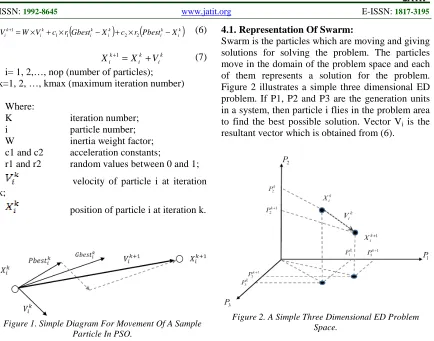
position of particle i at iteration k.

Figure 1. Simple Diagram For Movement Of A Sample Particle In PSO.

Inertia weight in PSO plays an important role because of its control on particle speed. Hence, a suitable selection of it is important. Equation (8) is the general selection of inertia weight. In current study the value of inertia weight decreases from 1.2 to 0.5 during a run time.

k

iteration iteration

W W W

W= − − × max

min max max

(8)

In (8), is the maximum number of

iterations while is the kth iteration which

is considered as current iteration in this paper.

4. PROPOSED METHODOLOGY

The current proposed PSO-based algorithm is developed to obtain an efficient solution for an Economic Dispatch (ED) problem. The optimized solution will give the best amount of power generation for each generation unit in terms of costs. Some definitions are made in the proposed algorithm as follows.

4.1. Representation Of Swarm:

Swarm is the particles which are moving and giving solutions for solving the problem. The particles move in the domain of the problem space and each of them represents a solution for the problem. Figure 2 illustrates a simple three dimensional ED problem. If P1, P2 and P3 are the generation units in a system, then particle i flies in the problem area to find the best possible solution. Vector Vi is the

resultant vector which is obtained from (6).

Figure 2. A Simple Three Dimensional ED Problem Space.

For a system with more than three generation units, we cannot demonstrate them in a 2-D paper because there is no Cartesian space available. However, we can consider systems with more than three dimensions theoretically to solve problems. In the current study, arrays and matrixes are the problem search space. For example, P[i][j] is a matrix of power generation in the proposed algorithm while i indicates the particle and j is the number of generation unit. For Figure 2, the dimension of problem will be 150×3, if we consider the number of particles to be equal to 150.

4.2. Fitness Function

To evaluate the proposed solutions by particles, we need to define a fitness function. The fitness function has to be able to determine which solution is better and more efficient after considering all the solutions obtained by the particles at each iteration. Normally the fitness function is being set to have the lowest possible value at an optimum point. In the current study, we also need to have the lowest possible value for the cost and transmission lost, hence the fitness function is proposed as follow:

∑

∑

∑ ∑

= = = =

− − × + = ng

j

ng

j

ng

i ng

j

j ij i d

j

j P P PB P

C L

1 1 1 1

530 where

L the value of fitness function;

Cj the cost function of generation unit j;

Pd the power demand by the loads;

λ _{coefficient of error;}

Pi and Pj the generated power by ith and jth

unit respectively.

Based on (9), the fitness function is generated by two parts: summation of costs and error in generation, which is the difference between the desired generation and real generation. The desired generation is the amount that can feed load demand

(Pd) and power transmission loss (4), but the real

generation is the summation of the generated power of all generation units. If those two numbers are not the same, the system will not work in an ideal situation and there will be a lack of feeding loads. In the best case, the absolute part in (9) will be

zero, therefore we set λ to a high value to magnify

any error. In this paper, the value of λ is equal to 100 and any small error will be mirrored in the value of the fitness function.

4.3. Proposed Algorithm Of PSO

Here, an algorithm based on particle swarm optimization is proposed to give a quick solution to solve economic dispatch problems. Unlike other PSO algorithms, in this method each single particle gives a solution to solve the main problem. In each generation of movement the best given solution by the particles is collected and that point in the problem space is called the global best. Personal best is the point that any particle by itself has experienced so far. Although these particles have the opportunity to search the full area of the problem space, missing some points in the problem space is inevitable because the vectors determine the direction of movement of each particle. Hence getting close to global best point might hold the particle around that point. However, the detected global best point is not necessarily the optimum solution to the problem. To overcome this, the acceleration factors of global best and personal best which are known as C1 and C2 have been adapted in a manner that let the particles search the problem space easier and with more efficient. The steps of the proposed algorithm are as shown below:

Step 1: receive the data of generation units’

characteristics, loss coefficients matrix B, and load demand from a text file. Initialize the positions for all the particles in the problem space randomly while the constraints of generation units are satisfied. X[i][j] holds the positions of particles in problem space while i indicates the particle and j is the generation unit.

Step 2: calculate the cost function (1) and

transmission loss matrix (4) based on loss

coefficients matrix B for each particle that gives a solution for the problem. Then an Error function is defined as a matrix to calculate the difference between the estimated power generation and

summation of demand load and as below:

E[i]=PG[i]-(Pd+Ploss[i]); (10)

Then the value of Error for each particle is divided among the number of generators to be shared between them. Step 2 is placed in an infinite for loop while the value of Error is less than a small

number ε which has been considered equal to

0.00000001 in the current algorithm.

Step 3: calculate the fitness function (9) based on

the obtained values for generation units from Step

2. Note that for each particle one fitness value

exists, hence we have a matrix with dimensions equal to the number of particles called L[i] where i indicates the particle.

Step 4: compare all values of L[i] matrix to find the

lowest value as the global best solution. This solution is saved in a matrix called Gbest[j] while its dimension is 1×j and j is equal to the number of the generation units. Since the movement part is not started yet, the personal best value of each particle is set to its current location and saved in a matrix called Pbest[i][j].

Step 5: Movement part: Modify the initial

velocity of each particle based on (11)

Vi[i][j]=Vmin+(((Vmax-Vmin)*Rand(0,1))); (11)

i=1,2,…,nop(number of particles) and

j=1,2,…,nod(number of dimensions)

While the number of dimensions demonstrates the number of generation units.

Step 6: A for loop which determines the number of

iteration starts from this step. Movement of particles starts by renewing the velocity of each particle based on (12).

Vk+1[i][j]=W×Vk

[i][j]+(r1*c1*(Gbest[j]-Xk[i][j]))+(r2*c2*((Pbest[i][j])-(Xk[i][j])))

(12)

Xk+1[i][j]= Xk[i][j]+ Vk+1[i][j] (13)

i=1,2,…,nop(number of particles) and

j=1,2,…,nod(number of dimensions)

ISSN: 1992-8645 www.jatit.org E-ISSN: 1817-3195

531 the inertia weight of velocity which is obtained by

(8), Xk[i][j] and Vk[i][j] are specifications of

particle i at iteration k, c1 and c2 are the global best acceleration factor and personal best acceleration factor respectively. Unlike existing PSO methods which took c1=c2=2, in current study they have different values as c1=0.2 and c2=2. In fact acceleration factors are tools to drag a sample particle to the place of global best point and personal best point. By decreasing the c1 as global best acceleration factor, particle has more degree of freedom in searching the problem space.

Calculating the new location of each particle of movement at iteration k+1 is the next aim of this step which is obtained trough (13).

Step 7: check the values of Xk+1[i][j] matrix to

make sure no generation unit violates its

constraints. If Xk+1[i][j] is not in range the value

will be set to either minimum when X<Pmin or maximum when X>Pmax.

Step 8: calculate the cost function (1), is

based on B-coefficient matrix (4) and value of fitness function matrix (9). Compare all values of

Lk+1[i] as the fitness matrix at iteration k+1 to find

the global best and then save the solution in Gbest[j]. The number of particle which generates Gbest[j] is saved as a number called OP means Optimum Particle. Compare the current fitness value of each particle at iteration k+1 with its value at iteration k through matrix L[i]. If the fitness value of any particle has decreased, the better solution would be replaced with former solution in matrix Pbest[i][j] which holds the best solution for each single particle.

Step 9: if the number of iteration reaches its

maximum, then go to Step 10. Otherwise, go to

Step 6.

Step 10: here Gbest[j] is the best solution of the

problem while j indicates the number of generation units. Also the particle which made the best solution has been saved in OP and can be obtained. Then by referring to the cost function which values are registered in cost[i][j] matrix, cost[OP][j] holds the cost of all generation units which are the optimum generation values.

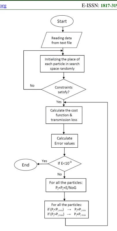
Figures 3 demonstrates the flowchart for initializing part of proposed algorithm.

Figure 3. Flowchart For The Proposed PSO-Based Algorithm: Initializing Part.

5. NUMERICAL RESULTS AND

DISCUSSION

Here, the results of four different case studies have been brought to verify the feasibility of the proposed PSO algorithm. In these cases, the obtained results are compared to existing PSO based and GA based results [10, 18, 19, 27]. At each case, under the same function of operation and algorithm, we performed 10 trials to make sure that the solution is not stammered in any local optimum point.

532 PSO method seems to be sensitive to the variation of weights and factors; hence in the present study different values for parameters have been set to find out how different factors and parameters can affect the swarm performance. However, the results presented only belong to the best set of parameters which lead the swarm to the optimum place.

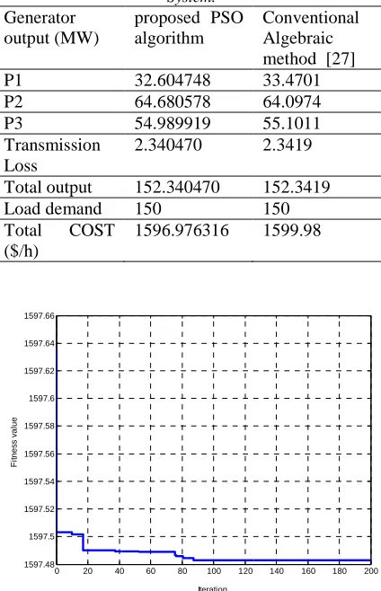
5.1. Case Study 1

Example 1: Three-Unit System: this case study has been adapted from [27] which is considered as a small system containing three thermal units. The system has the load demand of 150 MW. Table 1 shows the cost characteristics of three generators while matrix B is the loss coefficient matrix for the considered system.

Table 1. Cost Coefficients Of Three Units For Example 1.

Generation

unit no. ci bi ai Pmin Pmax

1 0.0080 7.00 200 10 85

2 0.0090 6.30 180 10 80

3 0.0070 6.80 140 10 70

B=

  

 

  

 

0.000179 0.000017

0.000028

0.000017 0.000228

0.000093

0.000028 0.000093

0.000218

The matrix Pg in this case has 3 columns based on three units and 150 rows based on the number of particles which is constant for all four cases. As it has been described the generation of P1, P2, and P3 are random and the dimension of the swarm is 150×3. The number of particles is normally assumed to be 100, but in the current study, the number has been increased to 150 to give the swarm more opportunity to search the problem space easier. However, for small cases we do not need many particles to find the optimum but in large scales, having a larger number of particles makes the swarm more capable to search the problem space faster and more reliable. The best results based on the proposed algorithm and existing results have been listed in Table 2. Figure 4 illustrates the convergence property of the proposed algorithm for example 1.

Table 2. The Best Obtained Results Of Three-Unit System.

Generator output (MW)

proposed PSO algorithm

Conventional Algebraic method [27]

P1 32.604748 33.4701

P2 64.680578 64.0974

P3 54.989919 55.1011

Transmission Loss

2.340470 2.3419

Total output 152.340470 152.3419

Load demand 150 150

Total COST

($/h)

1596.976316 1599.98

0 20 40 60 80 100 120 140 160 180 200

1597.48 1597.5 1597.52 1597.54 1597.56 1597.58 1597.6 1597.62 1597.64 1597.66

Iteration

F

it

n

e

s

s

v

a

lu

e

Figure 4. Convergence Property Of Proposed Algorithm For Example 1.

Results of Table 2 show an acceptable

improvement in the total cost of the system which demonstrates the ability of the proposed algorithm even in a small problem search space.

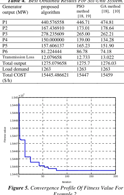
5.2. Case study 2

Example 2: Six-Unit System: this system includes six thermal generation units with characteristics given in Table 3 [28]. The system contains 26 buses and 46 transmission lines while the load demand is 1263 MW. Loss coefficients B matrix of the system is as follow:

Table 3. Cost coefficients for six-unit system for example 2.

Generation

unit no. ci bi ai Pmin Pmax

1 0.0070 7.00 240 100 500

2 0.0095 10.0 200 50. 200

3 0.0090 8.50 220 80. 300

4 0.0090 11.0 200 50. 150

5 0.0080 10.5 220 50. 200

ISSN: 1992-8645 www.jatit.org E-ISSN: 1817-3195 533 B=                     0.015000 -0.00020 -0.00080 -0.00060 -0.00010 0.00020 --0.00020 0.012900 -0.00060 -0.00100 -0.00060 0.00050 --0.00080 -0.00060 0.002400 0.000000 0.000100 0.00010 --0.00060 -0.00100 0.000000 0.003100 0.000900 0.000700 -0.00010 -0.00060 0.000100 0.000900 0.001400 0.001200 -0.00020 -0.00050 -0.00010 0.000700 0.001200 0.001700

In this case P1, P2, P3, P4, P5 and P6 generate the columns of Pg as generation matrix while the number of particles indicates the row number; hence the dimension of Pg is 150×6. Through the proposed algorithm the best solution of solving this problem are shown in Table 4. The obtained results satisfy the desired generating units’ constraints. The convergence property of the algorithm is illustrated in Figure 5.

Table 4. Best Obtained Results For Six-Unit System.

Generator output (MW) proposed algorithm PSO method [18, 19] GA method [18], [10]

P1 440.576558 446.71 474.81

P2 167.436910 173.01 178.64

P3 278.235609 265.00 262.21

P4 150.000000 139.00 134.28

P5 157.606137 165.23 151.90

P6 81.224444 86.78 74.18

Transmission Loss _{12.079658 12.733 13.022}

Total output 1275.079658 1275.7 1276.03

Load demand 1263 1263 1263

Total COST ($/h)

15445.486621 15447 15459

0 50 100 150 200 1.5445 1.5445 1.5446 1.5446 1.5447 1.5447 1.5448 1.5448 1.5449 1.5449

1.545x 10 4 Iteration F it n e s s v a lu e

Figure 5. Convergence Profile Of Fitness Value For

Example 2.

Table 4 shows that the proposed algorithm has more ability to find the optimal points in a search space compared to GA-based method in [18], [10] and also the proposed PSO-based method in [18, 19].

5.3. Case Study 3

Example 3: 15-Unit system: this system contains 15 thermal generating units and the characteristics of the units are given in Table 5 [29]. These

generation units have to support the load demand of 2630 MW plus the transmission loss with a B matrix as shown in the Appendix.

This example has quite a large problem search space compared to the previous examples, the P matrix of generation has the dimension of 150×15 where 150 indicates the number of the searching particles and 15 is the number of the generation units.

After applying the proposed algorithm to the problem, the results are shown in Table 6, which satisfy the constraints of the generation units. Figure 6 shows the convergence of values for the fitness function during iterations till the maximum iteration.

Table 5. Cost Data And Power Constraints Of 15-Unit

System For Example 3.

Gen. unit no. ci bi ai Pmin Pmax

1 0.000299 10.1 671 150 455

2 0.000183 10.2 574 150 455

3 0. 001126 8.80 374 20. 130

4 0. 001126 8.80 374 20. 130

5 0.000205 10.4 461 150 470

6 0.000301 10.1 630 135 460

7 0.000364 9.80 548 135 465

8 0.000338 11.2 227 60. 300

9 0.000807 11.2 173 25. 162

10 0. 001203 10.7 175 25. 160

11 0. 003586 10.2 186 20. 80. 12 0. 005513 9.90 230 20. 80. 13 0. 000371 13.1 225 25. 85. 14 0. 001929 12.1 309 15. 55. 15 0. 004447 12.4 323 15. 55.

Table 6. Comparative Results For 15-Unit System For

Example 3. Generator output (MW) proposed algorithm PSO method [18, 19] GA method [18], [10]

P1 455.000000 455.00 415.31

P2 455.000000 380.00 359.72

P3 130.000000 130.00 104.43

P4 130.000000 130.00 74.99

P5 286.412846 170.00 380.28

P6 460.000000 460.00 426.79

P7 465.000000 430.00 341.32

P8 60.000000 60.00 124.79

P9 25.000000 71.05 133.14

P10 37.560387 159.85 89.26

P11 20.000000 80.00 60.06

P12 80.000000 80.00 50.00

P13 25.000000 25.00 38.77

P14 15.000000 15.00 41.94

P15 15.000000 15.00 22.64

Transmission Loss

28.973234 30.908 38.278

Total output 2658.973234 2660.9 2668.4

Load demand 2630 2630.0 2630.0

Total COST ($/h)

534

0 20 40 60 80 100 120 140 160 180 200 3.255 3.26 3.265 3.27 3.275 3.28 3.285 3.29 3.295

3.3x 10 4 Iteration F it n e s s v a lu e

Figure 6. Convergence Property Of Fitness Value For

Example 3.

The results in Table 6 show that the proposed algorithm can find a better fitness value for the problem compared to the existing methods. The intense of convergence in Figure 6, also proves that the proposed algorithm is able to search the problem space move efficiently and faster.

5.4. Case study 4

Example 4: 40-Unit system: this system is a large-scale realistic Tai-power system which contains 40 generation units. The system is a mixture of oil-fired, gas-oil-fired, coal-oil-fired, diesel and combined cycle generating units [10]. The considered load demand for the system is 8550 MW. The

characteristics of the cost and generation

constraints for the generation units can be found in [10] but the B loss coefficient matrix is neglected because of limitation in space.

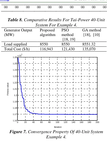
The results of applying the proposed algorithm to this example are shown in Table 7. Similarly, these results show improvement in the solution of the problem while satisfying all the constraints. Table 8 gives a comparative demonstration of the cost value for the proposed approach and previous efforts. The convergence property is shown in Figure 7.

Table 7. Output Generation (MW) Of Generation Units

For Tai-Power 40-Unit System For Example 4.

P1 P2 P3 P4 P5 P6 P7 P8 P9 P10

80. 00 120 .00 190 .00 24. 00 26. 00 68. 00 300 .00 300 .00 300 .00 300 .00

P11 P12 P13 P14 P15 P16 P17 P18 P19 P20

94. 00 94. 00 125 .00 356 .34 358 .73 355 .93 125 .00 500 .00 500 .00 242 .00

P21 P22 P23 P24 P25 P26 P27 P28 P29 P30

550 .00 550 .00 550 .00 550 .00 550 .00 550 .00 550 .00 10. 00 10. 00 10. 00

P31 P32 P33 P34 P35 P36 P37 P38 P39 P40

20. 20. 20. 20. 18. 18. 20. 25. 25. 25.

00 00 00 00 00 00 00 00 00 00

Table 8. Comparative Results For Tai-Power 40-Unit

System For Example 4.

Generator Output (MW) Proposed algorithm PSO method [18, 19] GA method [18], [10]

Load supplied 8550 8550 8551.32

Total Cost ($/h) 116,943 121,430 135,070

0 20 40 60 80 100 120 140 160 180 200 1.16 1.17 1.18 1.19 1.2 1.21 1.22 1.23 1.24 1.25 1.26x 10

5 Iteration F it n e s s v a lu e

Figure 7. Convergence Property Of 40-Unit System

Example 4.

Unlike previous examples and case studies, the results obtained in example 4 demonstrate improvement in the quality of the solution as well as finding a better optimum point for the problem.

6. CONCLUSION

In this paper, a new PSO-based algorithm is presented to solve Economic Dispatch (ED) problem of a power system. The solution process is tested on four different case studies from 3 generation unit to 40 generation unit. Although the algorithm is written in C code programming, the results are then transferred to MATLAB to make a drawing of convergence property of achieving the optimal point. Results and diagrams show improvements in the quality of solution which gives a better result in terms of cost issues. This fact proves that the proposed algorithm has more ability to solve both small and large case studies compared to the existing methods while the solution considers all the applied constraints of the generation units.

ACKNOWLEDGMENTS

ISSN: 1992-8645 www.jatit.org E-ISSN: 1817-3195

535

APPENDIX

The characteristics of the cost and generation constraints for the generation units for Example 4.

No. ci bi ai Pmin Pmax

1 0.03073 8.336 170.44 40 80

2 0.02028 7.0706 309.54 60 120

3 0.00942 8.1817 369.03 80 190

4 0.08482 6.9467 135.48 24 42

5 0.09693 6.5595 135.19 26 42

6 0.01142 8.0543 222.33 68 140

7 0.00357 8.0323 287.71 110 300

8 0.00492 6.999 391.98 135 300

9 0.00573 6.602 455.76 135 300

10 0.00605 12.908 722.82 130 300

11 0.00515 12.986 635.2 94 375

12 0.00569 12.796 654.69 94 375

13 0.00421 12.501 913.4 125 500

14 0.00752 8.8412 1760.4 125 500

15 0.00708 9.1575 1728.3 125 500

16 0.00708 9.1575 1728.3 125 500

17 0.00708 9.1575 1728.3 125 500

18 0.00313 7.9691 647.85 220 500

19 0.00313 7.955 649.69 220 500

20 0.00313 7.9691 647.83 242 550

21 0.00313 7.9691 647.83 242 550

22 0.00298 6.6313 785.96 254 550

23 0.00298 6.6313 785.96 254 550

24 0.00284 6.6611 794.53 254 550

25 0.00284 6.6611 794.53 254 550

26 0.00277 7.1032 801.32 254 550

27 0.00277 7.1032 801.32 254 550

28 0.52124 3.3353 1055.1 10 150

29 0.52124 3.3353 1055.1 10 150

30 0.52124 3.3353 1055.1 10 150

31 0.25098 13.052 1207.8 20 70

32 0.16766 21.887 810.79 20 70

33 0.2635 10.244 1247.7 20 70

34 0.30575 8.3707 1219.2 20 70

35 0.18362 26.258 641.43 18 60

36 0.32563 9.6956 1112.8 18 60

37 0.33722 7.1633 1044.4 20 60

38 0.23915 16.339 832.24 25 60

39 0.23915 16.339 834.24 25 60

40 0.23915 16.339 1035.2 25 60

REFRENCES:

[1] B. CHOWDHURY and S. RAHMAN, "A review of recent advances in economic

dispatch," IEEE Transactions on Power

Systems, vol. 5, pp. 1248-1259, 1990.

[2] B. Vanaja, et al., "Artificial Immune based Economic Load Dispatch with valve-point effect," 2009, pp. 1-5.

[3] S. H. Ling, et al., "Economic load dispatch: A new hybrid particle swarm optimization approach," 2008, pp. 1-8.

[4] A. Wood and B. Wollenberg, "Power generation, operation, and control. 1996," ed: John Wiley and Sons, New York.

[5] N. SINHA, et al., "Evolutionary programming techniques for economic load dispatch," IEEE transactions on evolutionary computation, vol. 7, pp. 83-94, 2003.

[6] A. P. Engelbrecht, Computational intelligence: an introduction: Wiley, 2007.

[7] Y. Shi and R. C. Eberhart, "Empirical study of particle swarm optimization," 2002.

[8] J. Kennedy and R. C. Eberhart, "Particle swarm optimization," 1995, pp. 1942-1948.

[9] A. BAKIRTZIS, et al., "Genetic algorithm solution to the economic dispatch problem," IEE proceedings. Generation, transmission and distribution, vol. 141, pp. 377-382, 1994. [10] P. Chen and H. Chang, "Large-scale economic

dispatch by genetic algorithm," IEEE

Transactions on Power Systems, vol. 10, 1995. [11] T. Yalcinoz, et al., "Economic dispatch solution

using a genetic algorithm based on arithmetic crossover," 2001.

[12] Y. Fukuyama and Y. Ueki, "An application of artificial neural network to dynamic economic load dispatching," 2002, pp. 261-265.

[13] T. YALCINOZ and M. SHORT, "Neural networks approach for solving economic dispatch problem with transmission capacity constraints," IEEE Transactions on Power Systems, vol. 13, pp. 307-313, 1998.

[14] T. Niknam, et al., "A new fuzzy adaptive particle swarm optimization for non-smooth economic dispatch," Energy, vol. 35, pp. 1764-1778, 2010.

536 [16] K. T. Chaturvedi, et al., "Particle swarm

optimization with crazy particles for nonconvex economic dispatch," Applied Soft Computing, vol. 9, pp. 962-969, 2009.

[17] Z. Zhisheng, "Quantum-behaved particle swarm optimization algorithm for economic load dispatch of power system," Expert Systems with Applications, vol. 37, pp. 1800-1803, 2010. [18] Z. L. Gaing, "Particle swarm optimization to

solving the economic dispatch considering the generator constraints," Power Systems, IEEE Transactions on, vol. 18, pp. 1187-1195, 2003. [19] C. C. Kuo, "A novel coding scheme for

practical economic dispatch by modified particle swarm approach," Power Systems, IEEE Transactions on, vol. 23, pp. 1825-1835, 2008.

[20] L. d. S. Coelho, et al., "Improved differential evolution approach based on cultural algorithm and diversity measure applied to solve

economic load dispatch problems,"

Mathematics and Computers in Simulation, vol. 79, pp. 3136-3147, 2009.

[21] T. Niknam, et al., "A new honey bee mating

optimization algorithm for non-smooth

economic dispatch," Energy, vol. 36, pp. 896-908, 2011.

[22] L. d. S. Coelho and V. C. Mariani, "An efficient cultural self-organizing migrating strategy for economic dispatch optimization with

valve-point effect," Energy Conversion and

Management, vol. 51, pp. 2580-2587, 2010. [23] M. Fesanghary and M. M. Ardehali, "A novel

meta-heuristic optimization methodology for solving various types of economic dispatch problem," Energy, vol. 34, pp. 757-766, 2009. [24] J. X. V. Neto, et al., "Improved

quantum-inspired evolutionary algorithm with diversity information applied to economic dispatch problem with prohibited operating zones," Energy Conversion and Management, vol. 52, pp. 8-14, 2011.

[25] C. T. SU and G. J. CHIOU, "A fast-computation hopfield method to economic dispatch of power systems," IEEE Transactions on Power Systems, vol. 12, pp. 1759-1764, 1997.

[26] K. Swarup and S. Yamashiro, "Unit

commitment solution methodology using

genetic algorithm," Power Systems, IEEE Transactions on, vol. 17, pp. 87-91, 2002.

[27] H. Saadat, Power System Analysis: McGraw-hill companies, 1999.

[28] H. Yoshida, et al., "A PARTICLE SWARM OPTIMIZATION FOR REACTIVE POWER AND VOLTAGE CONTROL CONSIDERING

VOLTAGE SECURITY ASSESSMENT,"

IEEE Trans. on Power Systems, vol. 15, pp. 1232-1239, 2001.