Recording and Measuring of Jaw Movements using a Computer Vision System

Recording and Measuring of Jaw Movements using a

Computer Vision System

Mahmoud Sedky Adly

Faculty of Dentistry Cairo University

Aliaa A.A. Youssif

Faculty of Computers and Information Helwan University

Ahmed Sharaf Eldin

Faculty of Computers and Information Helwan University

ABSTRACT

Human motion detection and analysis are important in many medical and dental clinics. Mandibular movements are very complex and difficult to detect by naked eyes. Detecting mandibular movements will aid in proper diagnosis, treatment planning and follow up. Many methods are utilized for measuring mandibular movements. However, most of these methods share the features of being very expensive and difficult to use in the clinic.

Using computer vision systems to track such movements may be considered one of the fundamental problems of human motion analysis that may remain unsolved due to its inherent difficulty. However, using markers may greatly simplify the process as long as they are simple, cheap and easy to use. Unlike other tracking systems, this system needs a simple digital video camera, and very simple markers that are created using black-white images that can be stick using any cheap double-sided bonding tape.

The proposed system is considered reliable and having a reasonable accuracy. The main advantages in this system are being simple and low cost when compared with any other method having the same accuracy.

Keywords

Motion analysis, image processing, mandibular motion, computer vision

1.

INTRODUCTION

Motion capturing of different parts of human body has evolved tremendously in many fields. Currently, human motion analysis plays an important role in many medical applications e.g., rehabilitation, medical examination, as well as in the analysis and optimization of movements of different parts of the human body.

Mandibular movements are considered one of the most complex movements in the body. The complexity of this movement makes it difficult to be detected by naked eyes. Recording of the mandibular movements is an important step in oral diagnosis especially in patients suffering from tempro-mandibular joint disorders [1]. The recording of these movements aid in determination of the underlying cause of the joint disorder whether it is dental, skeletal or muscular which eventually lead to selection of the most proper treatment plan and accurate follow up for the treatment progress [2].

Many techniques are used to measure mandibular movements. These include: 1) graphical method, 2) optoelectronic devices, 3) electromagnetic fields, 4) accelerometers, 5) video fluoroscopy and 6) ultrasound [1].

Graphical method which was presented by Ulrich and Walker consisted of a marking needle attached to a face bow, which was attached to the lower teeth and a marking disc or cardboard attached to the upper jaw or the head. It had the disadvantage of lacking definition and bulky equipments which is considered annoying to the patient [3].

The optoelectronic devices were first described by Karlsson. It was composed of light emitting diodes (LED), a position sensitive detector, and a computer. The main problem of this method was the rigid laboratory conditions [4].

Using electromagnetic sensors supported on the mandible was designed to capture and record the mandibular movement. However, it has a main problem of being affected by any electrical device. Also it was uncomfortable for patients and difficult to use in real dental facilities [5].

Accelerometers are electromechanical devices that measure acceleration of forces. These forces may be static, like the constant force of gravity, or they could be dynamic caused by moving or vibrating the accelerometer. They are undesirable for detecting mandibular movement as they do not produce stable recordings of the static position of the mandible [6, 7, 8].

To utilize video fluoroscopy in motion detection necessitates exposing the patients to ionizing radiation. Fluoroscopy works by applying a continuous flow of x-rays to obtain real-time moving images. This method is considered harmful to the patient and carrying the risk of carcinogenicity. So if the case is not an emergency it is recommended to use any other method [9, 10].

Measuring the mandibular movement by ultrasonic motion detector is a common method which measures distance by emitting ultrasonic pulses and determining the length of time it takes for the reflected pulses to return. We can then calculate a distance from the time and the known speed of sound. Unfortunately it had the disadvantage of being inaccurate and extremely sensitive to the environmental conditions [11, 12, 13].

All of the previous methods excluding the graphical method are sharing the features of being very expensive and difficult to use in common clinical scenarios.

2.

SYSTEM OVERVIEW

The movement measuring procedure is carried by following a sequence of steps that will calculate and track the position of the markers Figure 1.

Fig 1: The Main Structure of the System

The proposed system is a computer based system, where digital cameras are used to provide a video sequence, of either the Sagittal, Frontal, or Transverse plane, however if more than one plane is required in the same time we may use more than one digital camera. These planes are shown in Figure 2. The system is capable of analyzing the video sequence to measure the mandible movements.

Fig 2: Anatomical planes

3.

METHODOLOGY

In order to calculate the mandible range of motion the subject should be instructed to sit down on a chair, with the trunk positioned approximately 90o in relation to the transverse plane. The measurements are carried out by capturing the video while the subject’s lower jaw makes the motion with the

use of one or two normal classical digital cameras and the aid of at least two simple markers. Only one camera would be needed if the required analysis of movements in two-dimensional space, however at least two cameras are needed for three-dimensional space analysis. The subject should try not to move his head as much as possible but it is not a necessity to firmly hold his head by a head support unless he has any disorder that prevent him from controlling his neck. Similarly, the cameras can be held by hand as long as fast movements are avoided.

3.1

Marker Set:

Two simple markers are needed. Each marker is a simple six-sided cube shape that has square black and white images on its sides which consist of two-dimensional (2D) barcodes. Only black and white images that contain a square shape are used since the high contrast and their simplicity makes their detection easier.

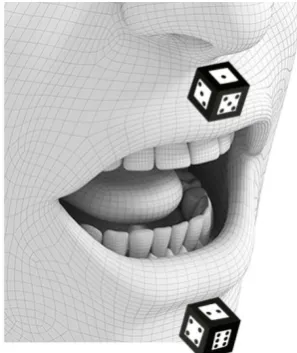
The markers can easily be created by printing the images then sticking them to a dice using a double-sided bonding tape. The first marker (primary marker) which is primarily employed to track the jaw should be fixed on the mandible as shown in figure 3. The second marker (secondary marker) should be fixed above the upper lip on the head and is used as a reference or a central point that is important in order to be able to calculate the mandibular movements and to compensate for any suspected head movement.

For example to calculate a transition we calculate the distance between the two markers before and after the transition then apply a simple subtraction operation. Similarly, we could compensate for the head movement by subtracting the movement of the primary marker from the secondary marker. Both markers are fixed using a double-sided bonding tape which is placed on one of the sides of the cube.

Fig 3: The view from the left camera after placing the markers

3.2

Camera Configuration:

To allow 3D construction, we will need to have each of the two cameras positioned in a manner that makes them capable of seeing at least two sides of the cube were one of the two sides is common between the two cameras. This condition can be satisfied by placing one camera on each side. Both the left and right cameras should form almost the same angle and be placed at approximately equal distance from the subject according to the marker size. The smaller its size the smaller the distance should be, however any distance would be fine

Video Preprocessing

Frames Thresholding

Line Detection

Connecting Line Segments

Corner Detection

Rectangle Construction

Rectangular Regions Extraction Detecting Cube Faces

Cube Construction

(although the smaller the better) as long as the markers are seen by the cameras and recognized by the system. It is preferable to place the cameras slightly higher than the markers. Figure 3 shows the view from the left camera.

3.3

Data Processing

3.3.1

Video preprocessing

The digital cameras video sequence is decomposed into frames, which will be preprocessed by smoothing in order to maximally reduce noise or instability. Some of the frames are automatically discarded according to a threshold function that determines the amount of movement occurred in these frames.

3.3.2

Frames Thresholding

To separate out the regions in the remaining frames we simply apply thresholding (image binarization) figure 4.

Fig 4: The frame after thresholding

3.3.3

Line Detection

The method used for line segment detection is based on an efficient hypothesis and test algorithm illustrated in [14]. This method is very accurate and fast enough to detect lines at frame rate on a standard workstation. As a consequence of utilizing this algorithm, the method will be blind to short line segments. But this is an advantage since we are only interested in line segments which will be suitable for tracking. Another advantage is that it is not needed to detect the entire length of a line segment in order to track it; instead this information is best obtained while tracking. The efficiency of this algorithm appear in using a sparse sampling of the image data to find candidate points (edgels) for lines then uses a grouper [15] to find line segments consistent with those edgels, which means that it does not demand to process every pixel in an image. To fit a line passing through a set of points, this approach works by randomly selecting two points (a sample), fit a line through these, and measure the support for the line. The support is the number of points that lie within a threshold distance of the line (the inliers). This process is repeated over a number of samples, and the line with the most support is then chosen. The line fit can then be improved by an orthogonal regression fit to the inliers. If there are several lines present, then there will be several lines with significant support. In general, the algorithm trades increased work in grouping for reduced work in edgel detection by only looking for edgels on a coarse grid of image pixels and then using this approach to find lines through these edgels. Since edgel detection is the dominant component this tradeoff results have a net gain which is speed. In our case, the performance of the algorithm improved dramatically, because we are only interested in binary images. On the other hand, the algorithm handles colored images by processing one of the three color channels and if an edgel is found in this color channel it is necessary to ensure that there is an approximately equally strong edgel at the same position in each of the remaining two channels. Reducing processing the three channels when using binary images decreases the algorithm’s running time dramatically.

3.3.4

Connecting Line Segments

After detecting line segments some of them may be connected. In this case we will need to merge them together. Two line segments are connected if and only if: both of them have the same orientation and they are neighbors.

Two line segments are neighbors if and only if: the difference between any of the end points of the first line segment and any of the end points of the second line segment is less than a threshold or there exists a set of connected line segments that connects both of them.

3.3.5

Corner Detection

After identifying straight lines within the image we then identify the points of intersections between these lines. All intersection points that have more than two lines crossing it are discarded. We search for corner points by picking a point of intersection from the set and try to find a clean corner. A clean corner is formulated when exactly two lines that are not parallel start from the same point (intersection point) and extends in only one direction. A corner line that extends in both ways can be common between more than one corner, which is not the case that we are looking for. If a corner is found we then start to search for another line that intersects with one of its lines. If we found an intersection we start to check whether it is a clean corner or not then repeat the process again until all the four corners are found.

Fig 5: (a) Two lines that form a pure corner (b) and (c) Two lines that does not form a pure corner since they are

common between more than one corner.

3.3.6

Rectangle Construction

A rectangle is constructed if the four corners that are found form a closed chain that consists of four lines.

Fig 6: (a) Four corners that form a closed chain consists of four lines (b) Two four corners that do not form a closed

chain.

3.3.7

Rectangular Regions Extraction

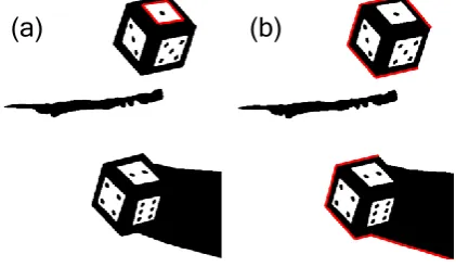
All detected rectangular regions are then extracted from the image.

Fig 7: The thresholded image after extracting all the rectangular regions.

3.3.8

Detecting Cube Faces Based on Orientation

We divide the detected faces into three groups based on orientation. This will help us identify each side and which side of the faces belongs to.

3.3.9

Cube Construction

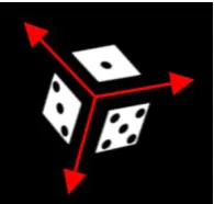
In this step, after all the faces are detected, their centers are calculated based on vertex pairs. All the faces are then checked to decide to which cube they belong. These faces are combined to form the cube. Finally, we calculate coordinates and pose for each cube by taking into consideration its faces.

Fig 8: Faces classification based on orientation

Fig 9: Faces information based on vertex pairs

Fig 10: Defining cube coordinates using its faces.

3.3.10

Cube tracking

In order to decrease processing we track the detected markers after being recognized. The detection process is performed in the first frame then the positions of the detected cubes are used to guide the detection process in the next frames. This means that the detection process is only performed in regions that contain a cube in the previous frame. To detect new markers that appeared in the view we perform the whole detection process periodically after a certain number of frames.

4.

EXPERIMENTAL RESULTS

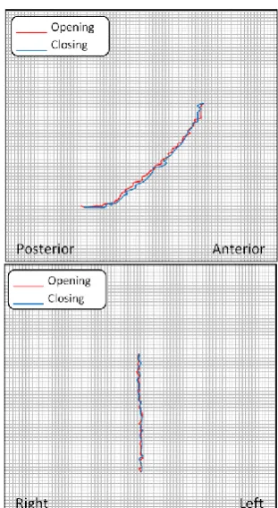
The mandibular movements of four subjects were collected using motion capture system. The subjects were instructed to perform ten opening-closing repetitions in order to acquire the mean movement values. No external forces or torques were applied and every action and general motion started from an initial position in which the mouth is fully closed. For all the subjects, the system was able to automatically detect the markers, calculate their 3D coordinates, analyze their orientation, and track their movements. Figures 11-14 show the coronal (frontal) / sagittal (lateral) view of the subjects.

Fig 14: Coronal (frontal) and Sagittal (lateral) views of jaw movement for a subject suffering from bilateral primary

osteoarthritis. It is usually associated with pain and tenderness on the joint area and crepitus (grating or crackling noise similar to the sound that is created when

one walks over gravel).

Fig 13: Coronal (frontal) and Sagittal (lateral) views of jaw movement for a subject suffering from Anterior Disc dislocation without reduction in the left tempro-mandibular

joint (The Shift begins to occur at approximately 20 mm) note the marked limiting in mouth opening. Fig 12: Coronal (frontal) and Sagittal (lateral) views of jaw

movement for a subject suffering from Anterior Disc dislocation with reduction in the tempro-mandibular joint

(note the sudden change in the curvature due transient locking of the disc during opening and sudden anterior sliding of the disc during closing). It is usually accompanied

To evaluate and compare the reliability of our method we used the graphical method to analyze the mandiblular movements in the frontal and the sagittal planes. To record the frontal movements we made an extra-oral apparatus that consisted of a metal frame holding a wax plate in a coronal direction which was attached to the upper anterior teeth. This frame was fixed by means of 2 wires attached to a piece of a u-shaped wax block emerging outward and holding the metal frame. The whole apparatus was fixed to the upper anterior teeth by sticky wax. A mandibular wire held the stylus of the tracking device and the wire was also attached to a piece of a wax block which is fixed to the lower teeth by means of sticky wax. For the recording of the sagittal movements the same device was used with a different orientation of the wax plate making it in a sagittal direction.

We compared the results of this manual experiment with the system’s results by calculating the root mean square error and there was no significant difference between them (P < 0.05).

5.

CONCLUSIONS and FUTURE WORK

This system was found to be reliable and having a reasonable accuracy. But the most important advantages we found about this system is being simple and having an extremely low cost when compared with any other method having the same accuracy. However, this method needs to be applied to patients suffering from other tempro-mandibular joint disorders which are considered rare. Examples of these rare diseases are: unilateral tempro-mandibular joint hypoplaia and

tumors of the tempro-mandibular joint (including chondroma, osteoma, osteosarcoma, osteoid osteoma and osteoblastoma) [16].

6.

REFERENCES

[1] Okeson JP. Management of temporomandibular disorders and occlusion. 6th ed. St Louis: Mosby Elsevier; 2007.

[2] Stuart CE. Diagnosis and treatment of occlusal relations of the teeth. Texas Dent J 1957; 75: 430-5.

[3] Walker WE. Movements of the mandibular condyles and dental articulation. Dent Cosmos 1896; 38: 573-83.

[4] Naeije M. Measurement of condylar motion: a plea for the use of the condylar kinematic centre. J Oral Rehabil. 2003;30:225-30.

[5] Wood WW. Medial pterygoid muscle activity during chewing and clenching. J Prosthet Dent. 1986;55:615-21.

[6] Mannini A, Sabatini A. Machine Learning Methods for Classifying Human Physical Activity from On-Body Accelerometers. Sensors 2010; 10: 1154-1175.

[7] Minami I, Oogai K, Nemoto T. Measurement of jerk-cost using a triaxial piezoelectric accelerometer for the evaluation of jaw movement smoothness. J of Oral Rehabilitation 2010; 37: 590–595.

[8] Holden JP, Selbie WS, Stanhope SJ. A proposed test to support the clinical movement analysis laboratory accreditation process. Gait Posture. 2003;17:205-13.

[9] Chen C, Lin C. A method for measuring three-dimensional mandibular kinematics in vivo using single-plane fluoroscopy. British Ins of Rad 2013; 42: 1259-1264.

[10]Yang Y, Yatabe M, Soneda K. The relation of canine guidance with laterotrusive movements at the incisal point and the working side condyle. J Oral Rehabil. 2000;27:911-7.

[11]Zharkova N, Hewlett N, Hardcastle W. Coarticulation as an Indicator of Speech Motor Control Development in Children: An Ultrasound Study. Human Kinetics, Inc. 2011; 15: 118-140.

[12]Hueber T, Benaroya E, Chollet G. Visuo-Phonetic Decoding using Multi-Stream and Context-Dependent Models for an Ultrasound-based Silent Speech Interface. Interspeech, Brighton 2009; 45: 640-643.

[13]Travers KH, Buschang PH, Hayasaki H, Throckmorton GS. Associations between incisor and mandibular condylar movements during maximum mouth opening in humans. Arch Oral Biol. 2000;45: 267-75.

[14]J. Clarke, S. Carlsson, and A. Zisserman. Detecting and tracking linear features efficiently. In Proc. British Machine Vision Conf., 1996.

[15]M. A. Fischler and R. C. Bolles. Random sample concerns us: A paradigm for model fitting with applications to image analysis and automated cartography. Comm. ACM, 24(6):381 395, 1981.

[16]Schiffman E, Anderson G, Fricton J. Diagnostic criteria for intraarticular T.M. disorders . Community Dent Oral Epidemiol 1989 ; 17: 252 – 257.

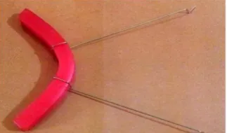
Figure 17: The metal frame holding a wax plate (used in the graphical method).

Figure 16: The lower u-shaped wax block with a stylus attached to it which is emerging outward to draw the

curve on the wax fixed to the metal frame.