Abstract – Occasional approach to thermal-physic task decision of grinding theory and numeral analysis based on imitation model realization by means of computer for the first time allow discovering the number of physical particular qualities of temperature field blank formation in this process.
It was established that temperature field has quasi-stationary occasional character.
It was discovered that availability of two criteria zones – the acceleration zone was defined by drastic temperature increase and the stabilization zone was conformed by constant level of temperature field formation – is typical for temperature field in the contact zone by grinding.
The statistic characteristics – two central moments of mathematical statistics: the mathematical waiting M(U) and the swing R(U) are offered for numeral evaluation of temperature field blank in the grinding zone.
Index Terms – Quasi-stationary temperature field, statistic characteristics statistic, heterogeneity.
I. INTRODUCTION
HE origin nature and character of temperature field blank during grinding was caused by abrasive grains influence. Abrasive grains’ interaction with working surface has occasional character because of probabilistic grains position character on the abrasive dick working surface. However nowadays this peculiarity of grinding process is difficult to be implemented in thermophysical models, bulit by MDM and FEA methods [1–4].
II. THERMAL MODELING OF GRINDING
Imitating thermal-physic model was designed to accommodate occasional interaction process of the abrasive disc and the blank working surface that includes in probabilistic formation of abrasive disc working surface [5].
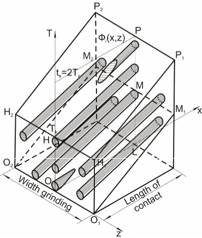
This model was realized in following scheme (fig. 1) – the blank scansion length equals the contact arc before the contact divided into i elementary sections (i=1….n). While the beginning of disc and blank interaction starts the first section enters the contact zone – its temperature field formation begins. Then, after some time pasts (h), the second section enters, and its temperature field formation
Manuscript received March 13, 2014.The reported study was partially supported by RFBR, research project No14-08-31064 мол_а.
A. A. Dyakonov is with the Engineering Department, South-Ural State University, Chelyabinsk, Russia (e-mail: [email protected]).
begins and so on up to n section.
Only thin layers of part blank are subject to sudden (impulsive) heat in the grinding zone. That is why during description the temperature field the geometry of part blank may be neglected, in other words for 3-D system it can be considered the case of half-space heating by sources moving on the surface. As used here the process of heat transmission mathematically comes to the second boundary problem for heat conduction equation in the half-space. Integral Decision is known for this linear model [5]:
(
)
( )
(
)
( ) ( )
( )
,4 , , 2
) , , , (
' ' 4
0 ' 3
' ' '
' 2 ' 2 ' 2
dz dx e
t t
t z x q dt
c t z y x U
t t
z z x x y
t
Di
− − + − + ×
×
∑ −
=
∫ ∫∫
χ
πχ
ρ
c – thermal diffusivity of material; ρ – density of material; χ
– thermal diffusivity of material; Di – the scope of i-sources – abrasive grain in XZT-system limited by surface
Фi (x, z)=0 (fig. 2); q – intensity of heat source.
It is rather complicated integral and not evaluated by famous special function.
As it is researched by many investigators the theory of high-speed sources can be used for grinding process offered by N.N. Ryikalin [6]. Using of this theory allows decreasing the number of independent coordinates and reducing integral equation for separately thermal source to following format:
, ) ) ( 4
) ( exp( )
( 2
1 ) , ,
( '
5 , 0
5 , 0
' 2 2 '
0 ' '
dz t t
y z z dt
t t
t q t
z y U
z
z l
l t
∫
∫
− −
+ − − −
=
χ πλ
U(y ,z, t) – the temperature in the moment t at the depth of y with z–coordinate in breadth; λ – thermal conductivity of material; lz – the length of abrasive grain blunting area.
Starting from the purposes of the research it is important to consider the temperature of thin layers of part blank to the moment of biting the next abrasive grain.
By S.N. Korchak [7] researched that for definition impulsive temperature it is required to consider thin layers of part blank within the limits of 0,05-0,002 mm as this depth is marginally allowed for scraping off material by single abrasive grain.
Alongside with this, change of temperature at the depth part blank surface in the following diapason 0,002– 0,010 mm are negligible as temperature drastic recession is observed at the depth of higher than 0,015 mm [7].
Simulated Stochastic Thermo-physical Model
of Grinding Process
Aleksandr A. Dyakonov, Member, IAENG
T
(1)
Fig. 1. The settlement circuit imitating thermal-physics model
Because of it y=0 and we can come to 2-D system. As the result dependence (2) come to the following equation:
. ) ) ( 4
) ( exp( )
( 2
1 ) ,
( '
5 , 0
5 , 0
' 2 '
0 ' '
dz t t
z z dt
t t
t q t
z U
z
z l
l t
∫
∫
− −
− − −
=
χ πλ
This dependence (3) describes the heating process from single thermal source. For realizing cooling-down calculation the dependence (3) computes with zero intensity of heat source (4).
( )
> ≤ =
. 0
; τ τ t t q t q
Taking into account expression (4) we have get the dependence describing cooling-down from single heat source (5).
. ) ) ( 4 exp( )
( 4 2
1 ) ,
( '
5 , 0
5 , 0
' 2
0 '
dz t t z dt
t t q t
z U
z
z l
l
∫
∫
− −
− −
=
χ πχ
πλ
τ
In the result taking into account dependences (3–5) the temperature from single heat source – abrasive grain – can be described by system of equations (6):
< < −
− ×
× −
< < −
− − ×
× −
=
∫
∫
∫
∫
− −
. )
) ( 4 exp(
) ( 4
) ( 2
1
; 0 ) ) ( 4
) ( exp(
) ( 2
1
) , (
1 '
5 , 0
5 , 0
' 2
0 '
'
' 5
, 0
5 , 0
' 2 ' 0
' '
t t dz t t z
dt t t t q
t dz t t
z z dt t t
t q
t z U
z
z z
z
l
l l
l t
τ χ
πχ πλ
τ χ
πλ
τ
The equation (6) describes the heating and cooling-down process cause of single heat source – abrasive grain taking into account flank flow-out at circle breadth.
However, using of this integral for calculations involves difficulties even by computer.
Analysis of the literature concerning thermal physics of solids makes clear that integral (3) can be expressed by special functions: error function erf (x) and integral exponential function Ei:
• error function erf (x):
∫
−= x x
dx e x
0
. 2
) (
erf 2
π
• integral exponential function Ei:
∫
∞ − − =
1
. )
(x e u du
Ei xu n
The meanings of these functions are learned [8]. As the result we have get:
. 4
) 5 , 0 ( 4
5 , 0 4
) 5 , 0 (
4 5 , 0 4 5 , 0 4
5 , 0 )
, (
2 2
−
− − +
+
−
× + +
−
+
+
=
t z l Ei t
z l t
z l Ei
t z l t
z l erf t
z l erf t q t z U
z z
z
z z
z
χ πχ
χ
πχ χ
χ π
λ χ
q – intensity of heat source; λ – thermal conductivity of material; a – the half of length heat source (a=0,5lz); erf(x) – error function; Ei – integral exponential function, z – coordinate of source endwise Z; x – thermal diffusivity of material.
Using the method of reflected sources [8] to describe cooling-down process is used equation for heating (9) from which analogue equation subtracted with t:
Fig. 2. The principle scheme of thermal sources influence
(6)
(3)
(7)
(8)
(9) (4)
. ) ( 4 ) 5 , 0 ( ) ( 4 5 , 0 ) ( 4 ) 5 , 0 ( ) ( 4 5 , 0 ) ( 4 5 , 0 ) ( 4 5 , 0 ) ( 4 ) 5 , 0 ( 4 5 , 0 4 ) 5 , 0 ( 4 5 , 0 4 5 , 0 4 5 , 0 ) , ( 2 2 2 2 − − − − − + + − + − − + + + − − + − + × × − − − − × × − + + − × + + + − + + = τ χ τ πχ τ χ τ πχ τ χ τ χ π λ τ χ χ πχ χ πχ χ χ π λ χ t z l Ei t z l t z l Ei t z l t z l erf t z l erf t q t z l Ei t z l t z l Ei t z l t z l erf t z l erf t q t z U z z z z z z z z z z z z
As the result equation (6) can be signed by equations system (11): < − − − × × − − + + − + − × × − + + − − + − + − − − − − − + + + − + + − + + < < − − − + + + − + + + − + + = . ) ( 4 ) 5 , 0 ( ) ( 4 5 , 0 ) ( 4 ) 5 , 0 ( ) ( 4 5 , 0 ) ( 4 5 , 0 ) ( 4 5 , 0 ) ( 4 ) 5 , 0 ( 4 5 , 0 4 ) 5 , 0 ( 4 5 , 0 4 5 , 0 4 5 , 0 ; 0 4 ) 5 , 0 ( 4 5 , 0 4 ) 5 , 0 ( 4 5 , 0 4 5 , 0 4 5 , 0 ) , ( 2 2 2 2 2 2 t t z l Ei t z l t z l Ei t z l t z l erf t z l erf t q t z l Ei t z l t z l Ei t z l t z l erf t z l erf t q t t z l Ei t z l t z l Ei t z l t z l erf t z l erf t q t z U z z z z z z z z z z z z z z z z z z
τ
τ
χ
τ
πχ
τ
χ
τ
πχ
τ
χ
τ
χ
π
λ
τ
χ
χ
πχ
χ
πχ
χ
χ
π
λ
χ
τ
χ
πχ
χ
πχ
χ
χ
π
λ
χ
There are no difficulties concerning calculation of equation system (11) both by computer and by hand.
The elementary section application is based on the theory of high-speed sources [6]. According this theory during high-speed processes the heat secretion happens only in the transverse direction to cutting speed vector. And in the direction of speed vector, taking into account its high order, the convection flow-out takes place.
Using the Monte-Carlo method the occasional analysis of temperature field formation was realized [7] – according to the given initial data n versions of abrasive disc work surfaces formatted and for each version the temperature field calculations in the given time moments are performed.
III. RESULTS AND DISCUSSION
Occasional approach to thermal-physic task decision of grinding theory and numeral analysis based on imitation model realization by means of computer for the first time allow discovering the number of physical particular qualities of temperature field blank formation in this process.
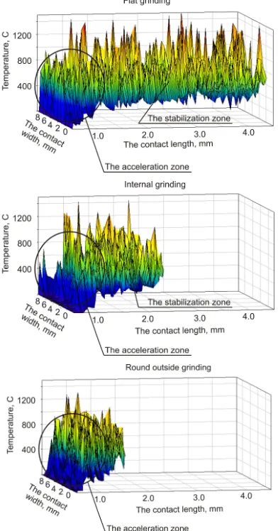
The fig. 3 illustrates, there is the contact length at the axis of absciss and there is the grinding width at the axis of ordinates. It allows to monitor the nature of temperature field formation in the contact zone both in the cutting moment by grains (maximal temperature tops) and in the «rest» time until the next grain enters when the material is getting cold. At the graphs you can see the critical fluctuation points of temperature field – maximal and minimal temperature. Furthermore, the temperature field has the not stational and irregular character both at the contact length and the contact width, in other words the temperature fluctuations move to the area of higher temperature at time.
For the all materials the maximal temperatures could reach and even exceed melting-point and independently on processing kind. It is the demonstration of one assumption influence using in thermal-physics model, namely metal – isotope and while calculating its phase transformations during heat spread process (latent warmth melting) are not taken into account. It allows avoiding nonlinear thermal conductivity differential equation. It is very important to solve this problem for investigations those concerned with determination of structural changes in the surface layers. This problem is not discussed in the present report. Moreover, A.A. Koshin [8] represents that material melting temperature is available only on the surface, and in the significant volumes of surface layers determining the quality of processing this effect is not monitored.
Thus, the maximal temperature that appears in the thin surface layers, could reach physically the melting-point and since this time the getting cold happens whish is describing in the designed thermal-physics model.
[image:3.595.71.290.48.250.2]The particular cases are recognized after analyzing the great number of temperature field diagrams. So, for the all examined material marks independently on the grinding kind, the sudden increases and drops interchange in the temperature of getting cold is monitored in the high temperature zone. It is concerned with nonlinear changes of dependence “Solidity-Temperature” for that diapason in
Fig. 3. The temperature field blank kind by grinding (10)
Fig. 4. Characteristic sites of temperature field blank formation which the meanings of material solid characteristics (σi) and intensity heat sources (q) are not taking into account.
Comparing the given temperature fields for different kinds of grindings it could be established that while the contact length increases the temperature gradient increases too. So, during the round outside grinding of carbon steels the average temperature gradient is 380 °C, during the flat grinding – 650 °C and during the internal grinding – 310 °C. On the other hand, the temperature increase is not proportionate to contact length increase as correlation of the contact length at flat and outside round grinding at average technological conditions is 3,8 : 1, and correlation of temperature is 1,7 : 1. This event could be explained by availability of acceleration and stabilization zone (fig. 4) at temperature field. The drastic temperature increase that practically equals the maximal temperature happens on the contact length that is 1 mm not dependently on grinding kind, and the future development of temperature field happens at stabilization dependence relatively to abscissa axis. However the part of acceleration zone of the contact length for every kind is not similar, for example, for the round outside grinding it is 100 %, for the internal grinding – 62 %, for the flat grinding – 25 %.
Consequently the temperature field blank by grinding possesses of two criteria zones: the zone of drastic temperature increase (the acceleration zone) and the stabilization zone.
Modification of the given diagrams into the line level diagrams (fig.5) allows to monitor distribution and heterogeneity of temperature field blank in the contact zone.
Fig.4 illustrates quasi-stationary temperature field is created in the results of the frequent influence of abrasive grains on the stabilization zone that is 800 ºС, due to occasional grinding process temperature pulsation happens in the interval of 200–1400 ºС.
The main particular quality of temperature field, which was idealized vastly by investigators [5], is occasional character of its formation. Starting from this, to evaluate temperature field in the contact zone the application of mathematical statistics is required as the average of temperature in this case, obviously disfigures the real situation.
Two central moments of mathematical statistics are implemented for evaluation:
M (U) – mathematical temperature waiting in the considered interval at the contact length;
R (U) – swing of temperature relatively to mathematical waiting in the considered interval at the contact length.
Two-parameter evaluation system was realized by computer statistics prognostication STATISTICA 6.0. To determine mathematical waiting M (U) and swing R (U) in every interval at the contact length the meanings of temperature at the contact width included in this interval are considered.
[image:4.595.335.517.373.487.2]The example of trusting temperature field evaluation at flat grinding of AISI304 is illustrated on the fig. 6. The results confirm the necessity of two-parameter evaluation system as the swing in the dependence on the considered contact length could obtain 220–980 ºС. The analyzing of the graphs allows concluding that temperature field blank possesses additional particular qualities besides indicated earlier.
[image:4.595.313.536.617.762.2]Fig. 6. The temperature swing interval statistics Fig. 5. The line level heterogeneity diagram of temperature
The temperature swing obtains the different meanings on the individual contact length in which connection its meaning decreases while the contact length increases (Table I).
IV. CONCLUSION
Occasional approach to thermal-physic task decision of grinding theory and numeral analysis based on imitation model realization by means of computer for the first time allow discovering the number of physical particular qualities of temperature field blank formation in this process.
It was established that temperature field has quasi-stationary occasional character.
It was discovered that availability of two criteria zones – the acceleration zone was defined by drastic temperature increase and the stabilization zone was conformed by constant level of temperature field formation – is typical for temperature field in the contact zone by grinding.
The statistic characteristics – two central moments of mathematical statistics: the mathematical waiting M (U) and the swing R (U) are offered for numeral evaluation of temperature field blank in the grinding zone.
REFERENCES
[1] F. Klocke “Modelling und simulation in grinding,” 1st European Conference on Grinding, Berichte, bd. 8, 2003, ss. 1–27.
[2] S. Malkin, C. Guo “Thermal Analysis of Grinding,” CIRP Annals -
Manufacturing Technology, vol. 56, Is. 2, 2007, pp. 760–782.
[3] A. Mamalis, G. J. Kundra´k, D. E. Manolakos “Thermal Modelling of Surface Grinding Using Implicit Finite Element Techniques,”
International Journal of Mechanical Sciences, vol. 21, 2003, pp.
929–934.
[4] D. L. Scuratov [et al.] “Mathematical modelling and analytical solution for workpiece temperature in grinding,” Applied
Mathematical Modelling, vol. 31, 2007, pp. 1031–1047.
[5] A. A. D`yakonov “Improvement of grinding speeds by assessing the
machinability of materials,” Russian Engineering Research, vol. 32,
Issue 7-8, 2012, pp. 604-607.
[6] N. N. Ryikalin “Account and modeling of a temperature field of a product at grinding,” The bulletin of mechanical engineering, vol. 1, 1963, pp. 74–77.
[7] G. Karslou “The Thermal conductivity,” Science, Moscow,1964. [8] A. A. Koshin “Research of physical communications at grinding,”
The Processing of metals, vol. 1, 1997, pp. 22–25.
[9] S. N. Korchak “Productivity of process of grinding of steel details,” Mechanical engineering, Moscow, 1974.
TABLEI
THE TEMPERATURE SWING INTERVAL STATISTICS
Number of the site
I II III
The grinding kind
R (U), 0С
Round outside 530 500 421
Internal 550 390 –