Abstract—A time conservative two–dimensional flow solver has
been developed and validated for solving the filtered Navier-Stokes equations. The method is based on a multi-block structured quadrilateral mesh. The conservation element and solution element (CE/SE) method, which is a second-order scheme in space and time, is employed. A simple two-level multi-grid method is implemented for convergence acceleration. Several cases with a wide range of flow conditions have been computed to verify the accuracy of method and demonstrate its effectiveness. An unsteady Euler solution is obtained for a forward facing step to demonstrate the robustness of the numerical scheme. The Navier-Stokes solver is validated with a laminar flow over a flat plate test case. A large eddy simulation (LES) is performed for a spatially evolving mixing layer and compared with the results of a high-order scheme. The subgrid scales of turbulence are modeled with the Smagorinsky subgrid scale (SGS) model. The results using the present 2nd order scheme are in good agreement with other published results, showing high accuracy and high resolution, comparable those of high-order numerical schemes.
Index Terms—CE/SE method, computational aero-acoustics,
large eddy simulation, multi-grid.
I. INTRODUCTION
One of the challenges in computational fluid dynamics (CFD) development is in the computational aero-acoustics (CAA) field. The modeling requirement of aeroacoustics problems is substantially different from traditional fluid dynamics problems. The acoustical signals are typically much smaller than those of mean flow disturbances and hence require much higher resolution, and lower dissipations from computational methods. There are two approaches used to obtain accurate results for CAA problems. The first one employs standard CFD methods with much finer meshes and the second one employs high-order numerical schemes.
Standard second-order CFD schemes are generally too dissipative to adequately compute and simulate aeroacoustics
Manuscript received March 2, 2007.
O. Aybay is with School of Engineering Department, University of Durham, DH1 3LE, Durham, UK (phone: +441913342412; fax: +441913342377; e-mail: [email protected]).
L. He is with School of Engineering Department, University of Durham, DH1 3LE, Durham, UK (e-mail: [email protected]).
problems [1]. The numerical schemes should resolve acoustic waves with low dispersion and low dissipation.
High-order numerical schemes have been widely used for CAA applications. However, they attend to have difficulties in simulating regions with the steep flow gradients (e.g. around shock waves). The major drawbacks of the high-order schemes are the lack of a shock-capturing property and difficulty to deal with the complex geometry. Spurious oscillations are frequently observed in the steep regions of the shock [2]. These oscillations can be dampened by employing low-order smoothing in the vicinity of steep pressure gradients. However, the smoothing will prevent the numerical schemes suitability for general applications and result in loss of accuracy [3]. The other difficult aspect of the high-order scheme is in application of the boundary conditions. The order of the schemes tends to be reduced on the boundaries which results in more complicated boundary condition treatments and again reduction of accuracy.
Therefore, there is a need for further development to address these issues associated with the standard second-order CFD schemes and the high-order schemes. The approach taken here is to further develop higher resolution, low dissipation second-order scheme, aimed at solving complex unsteady aerodynamic and aero-acoustics problems with higher accuracy. The time conservative finite volume scheme, which is a good compromise between them, has been employed. This method is known as conservation element and solution element (CE/SE) method and originally proposed by Chang [4] at NASA Glenn Research Center. In this method, spatial and temporal discretizations are unified, flow variables and their spatial derivatives are treated as unknowns and non-reflecting boundary conditions are imposed with a little programming effort. The CE/SE scheme was modified for a two-dimensional case using regular structured quadrilateral meshes by Zhang and Yu [5]. A generalized quadrilateral mesh extension can be found in Zhang et al. [6]. This extension is employed in this study with some modifications.
In the time conservative finite volume method, time-marching can be done explicitly. The time step is limited by the smallest mesh size due to the stability restriction. In the present work, a simple multi-grid method is developed and implemented in the time conservative scheme to accelerate the convergence.
Time Conservative Finite Volume Method for
Large Eddy Simulations
O. Aybay and L. He
II. GOVERNING EQUATIONS
Flow variables simulated by LES are decomposed as follows
sgs Φ ′ + Φ = Φ (1)
where Φ is large scale or resolved scale and
sgs
Φ ′ is small scale or subgrid scale. For compressible flows Favre-filtering is a common approach. Any other filtering approach will introduce more complicated subgrid scale terms in the governing equations. A Favre-filtered variable is defined as:
ρ ρΦ =
Φ~ (2)
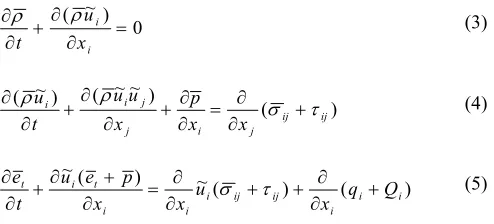
The continuity, momentum and energy equations of Favre-filtered, unsteady and compressible Navier-Stokes equations are expressed as:
0 ) ~ ( = ∂ ∂ + ∂ ∂ i i x u t ρ ρ (3) ) ( ) ~ ~ ( ) ~ ( ij ij j i j j i i x x p x u u t
u ρ σ τ
ρ + ∂ ∂ = ∂ ∂ + ∂ ∂ + ∂ ∂ (4) ) ( ) ( ~ ) ( ~ i i i ij ij i i i t i
t q Q
x u x x p e u t e + ∂ ∂ + + ∂ ∂ = ∂ + ∂ + ∂ ∂ τ σ (5)
where
σ
ij,τ
ij,q
iandQ
i are resolved viscous stress tensor, subgrid stress tensor, resolved heat flux and subgrid heat flux, respectively.The resolved scales can be solved directly by Favre-filtered Navier-Stokes equations whereas the subgrid scales have to be modeled. In this study due to its simplicity the classical Smagorinsky subgrid scale (SGS) model is employed. The resolved viscous stress tensor is defined as:
) ~ 3 1 ~ ( ~
2 ij kk ij
ij µ S S δ
σ = − (6)
where
ij
δ is the Kronecker delta and
ij
S~ is the Favre-filtered strain rate tensor given by:
) ~ ~ ( 2 1 ~ j i i j ij x u x u S ∂ ∂ + ∂ ∂ = (7)
The resolved heat flux is defined as:
x T C
qi p
∂ ∂ = ~ Pr ~ µ (8)
where CP, µ~ and Pr are specific heat at constant pressure,
molecular viscosity and Prandtl number, respectively. The subgrid stress tensor is modeled as:
ij M I ij kk ij M R
ij C ρ S S S δ C ρ S δ
τ 2 2~2
3 2 ) ~ 3 2 ~ 2 ( ~ ∆ − − ∆ = (9)
The subgrid heat flux is modeled using a temperature gradient approach i t M R p i x T S C C Q ∂ ∂ ∆ = ~ Pr ~ 2 ρ (10) where ij ij
M S S
S~ = 2~ ~ and CR = 0.0324 and CI = 0.00575 are
the Smagorinsky model constants and ∆ is the filter width defined as ∆ = ( ∆x, ∆y)1/2.
The Sutherland law is also used for molecular viscosity, µ~ and the governing equations are closed by the perfect gas relation.
Navier-Stokes computation without turbulent flow has been carried out by replacing all filtered variables with their unfiltered forms and setting the subgrid stress tensor and the subgrid heat flux terms to be zero. Furthermore, for Euler computation the viscous stress tensor has been set to zero.
III. NUMERICALMETHOD
The spatial and temporal discretizations are unified in the time conservative finite volume method. Temporal and spatial discretizations are performed using the same method. Discretization of the CE/SE method can be found in details in the literature [4]. In the present study, the numerical scheme given by Zhang et al. [6] was employed with some modifications. Instead of using overlapping nonstaggered mesh, non-overlapping staggered mesh was employed. The scheme alternates between the vertices full circle dots and the centers square dots in Fig. 1. Simple and more precise boundary conditions can be imposed. Furthermore, local flux conservation around the boundary and global flux conservation is guaranteed by this modification.
[image:2.595.47.294.319.431.2]The flow variables are assumed smooth inside the control volume. Fluxes and the flow variables are approximated by the Taylor series expansion (i.e. second-order linear distribution). For each grid mesh point, the flow variables and
derivative of the flow variables are stored and updated. At time
tn, flow variables at the full circle dots and square dots are assumed to be known in Fig. 1. Local flux conservation is used to update the flow variables at square dots at tn+1/2 and then to update the flow variables at full circle dots at tn+1. Boundary conditions are only imposed at full circle dots. The other modification is related to derivative of the flow variables. Instead of performing a spatial translation of the quadrilateral given by Zhang et al. [6], a central difference method was used between mesh points to calculate the derivative of the flow variables. Better numerical dissipation control is achieved by this modification, which is very important for problems with a highly non-uniform mesh.
IV. TWO-LEVEL MULTIGRID METHOD
A simple multigrid method at two-level proposed by He [7] is employed to accelerate the present explicit time marching scheme. For one level, temporal change of the flow variables is defined as:
f f f f n n
V R t U
U
∆ ∆ = −
+ )
( 1 (11)
where the subscript f denotes fine mesh, ∆tf is the allowable time
step and Rf is the net flux for the finite volume on the fine mesh.
For the two-level time integration method the solution is marched first on the fine mesh and then on the coarse mesh. The overall time step is much larger than the one level temporal change and the accuracy of the solution is controlled by the fine mesh. Therefore, the temporal change of the flow variables on the fine mesh is
c c c f f f f n n
V R t V R t U
U
∆ ∆ + ∆ ∆ = −
+
)
( 1 (12)
where the subscript c denotes coarse mesh, ∆tc is the allowable
time step and Rc is the net flux for the finite volume on the
coarse mesh. Implementation of this simple multigrid method is much easier than the conventional one. More details of the two-level multigrid method can be found in the literature [7].
V. RESULTS AND DISCUSSION
A. Flow over a Forward Facing Step
A supersonic flow over a forward facing step problem is solved to demonstrate the robustness of the present numerical scheme. This benchmark problem is the same as the one studied by Woodward and Colella [8]. It was also used by Giannakouros and Karniadakis [9]. The present computations are carried out by using a multi-block Euler solver. The computational domain is 3.0 m × 1.0 m. Uniform structured mesh is used with ∆x = 0.0125 m and ∆y = 0.01 m grid spacing
x
y
0 0.5 1 1.5 2 2.5 3
0 0.5 1
(a) t = 2.8 × 10⁻² s
x
y
0 0.5 1 1.5 2 2.5 3
0 0.5 1
[image:3.595.311.523.88.280.2](b) t = 4.0 × 10⁻² s Fig. 2 Density contours with 30 levels
in the x and y directions, respectively. The free stream Mach number is 3.0, the stagnation pressure is 105 Pa and the stagnation temperature is 300 K. These flow conditions are imposed on the left-hand boundary as the supersonic inlet boundary condition. The upper and the lower boundaries are an inviscid wall, where a slip boundary condition is imposed. Lastly, the supersonic outflow boundary condition is applied on the right-hand boundary.
Calculated density profiles with 30 contours at t = 2.8 × 10⁻² s and t = 4.0 × 10⁻² s are shown in Fig. 2(a) and Fig. 2(b), respectively. The Mach stem in the lower wall, expansion fan at the corner of the step and the interaction between the reflected shocks with rarefaction waves are accurately calculated with high resolution. According to Woodward and Colella [8], without applying special numerical treatment at the corner of the step, calculations would be affected by large numerical errors. However, the present calculations are carried out without employing any special treatment at the corner of the step and no numerical oscillations are detected around a shock wave.
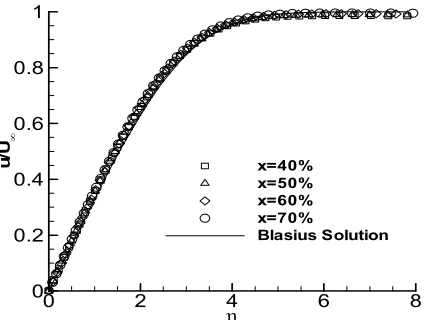
B. Laminar Flow over a Flat Plate
Calculated streamwise velocity profiles for two-grid time integration results are compared with the Blasius solution in Fig. 3. It is observed in the figure that the streamwise velocity profiles are in good agreement with the Blasius solution.
where
x x y
Re =
η and
µ ρux x=
Re
Development of the laminar boundary layer on the flat plate can be seen in Fig. 4 and the variation of calculated local skin friction coefficient, Cfx on the flat plate is compared with the
Blasius solution in Fig. 5 for the single and two-level multigrid methods. Similarly, these results are in good agreement with the Blasius solution. The local skin friction coefficient is defined as:
2 5 .
0 ∞ ∞
=
U
C w
fx ρ
τ where
0
=
∂ ∂ =
y w
y u µ
τ (13)
The comparison of residual history for laminar flow over a flat plate is presented in Fig. 6. The comparison shows the improvement by employing a multigrid application with respect to a single grid calculation. The steady state is reached when the residual dropped approximately 4.5-5 orders of magnitude and due to the use of the larger time step the steady state can be quickly reached in multigrid solutions without losing any significant accuracy.
η
u
/U
∞
0 2 4 6 8
0 0.2 0.4 0.6 0.8 1
x=40% x=50% x=60% x=70%
[image:4.595.312.533.320.484.2]Blasius Solution
Fig. 3 Axial velocity distribution at 40%, 50%, 60% and 70% of the flat plate for the two-grid time integration method
x
y
0 0.2 0.4 0.6 0.8 1
0 0.1 0.2 0.3
Mach: 0.02 0.04 0.06 0.07 0.09 0.11 0.13 0.15 0.16 0.18 0.20 0.22 0.24 0.25 0.27
Fig. 4 Laminar boundary layer development and velocity vectors on the flat plate
x
C
fx0 0.2 0.4 0.6 0.8 1
0.05 0.1 0.15
Single-Grid Two-Grid Blasius Solution
Fig. 5 Skin friction coefficient along the flat plate
Number of Time Steps
L
o
g
(R
e
s
id
u
a
l)
10000 20000 30000 40000 50000
-6 -5 -4 -3 -2
Single-Grid Two-Grid
Fig. 6 Comparison of residual history of momentum in x
direction for laminar flow over a flat plate
C. 2-D Mixing Layer
A two-dimensional spatially evolving mixing layer problem is solved. This test case was also studied by Uzun [10] and Bogey [11]. In-flow hyperbolic tangent velocity profile is expressed as:
−
+ + =
) 0 ( 2 tanh 2
2 )
( 1 2 2 1
w y U
U U U y u
δ (14)
where U1 = 50 m/s and U2 = 100 m/s are the lower and upper
velocities, respectively. δω(0) = 1.6 × 10⁻³ m is the initial
vorticity thickness. The transverse velocity with random perturbation is given by:
∆ −
+
=∈
2 0 2 2
1 exp
2 )
(
y y U
U y
[image:4.595.53.266.425.585.2] [image:4.595.59.265.627.711.2]where α = 0.0045, ∆y0 is the minimum grid spacing in the y
direction and ∈ is a random number between -1 and 1. The non-reflecting boundary conditions are imposed at the upper and the lower boundaries. The convective Mach number which measures the intrinsic compressibility of a mixing layer [12] is defined as:
074 . 0 2
1
2 − =
=
∞ c
U U
Mc (16)
where c∞ is the free stream speed of sound. The Reynolds number based on the initial vorticity thickness and velocity difference is given by:
5333 ) )(
0 (
Re = 2− 1 =
ν δω ω
U
U (17)
The mesh density is 625 × 301 in the x and y directions, respectively. The computational domain lies between
m 4 . 0
0≤x≤ and −0.16m≤ y≤0.16m . The mesh is uniform in the streamwise direction whereas in the transverse direction exponential grid stretching is applied. The minimum grid spacing is about 0.16δω(0) at y = 0 and the maximum grid
spacing around the lower and upper boundaries is 3.0δω(0).
In Fig. 7, instantaneous vorticity contours are shown and vortex pairing at different locations can be observed. The vorticity thickness evaluation is shown in Fig. 8. After the initial transients, the vorticity thickness grows linearly. The spreading rate parameter is given by [13]:
09 . 0 ) ( ) (
5 . 0
1 2
2
1 =
∂ ∂ −
+ =
x x U
U U U
S δω (18)
The range of reported experimental results for the parameter
S is from S ≈ 0.06 to S ≈ 0.11 [13]. The parameter S predicted by Smagorinsky model is within the range of experimental values. The normalized Reynolds stresses are defined as:
2 1
2 )
(U U
u u xx
− 〉′ ′ 〈 =
σ ,
2 1
2 )
(U U
v v
yy −
〉 ′ ′ 〈 =
σ
2 1
2 )
(U U
v u
xy −
〉 ′ ′ 〈 =
σ (19)
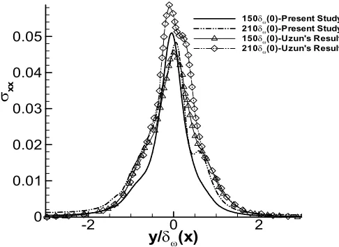
where 〈〉denotes time-averaging. In Figs. 9, 10 and 11 the turbulence intensities are compared with Uzun’s normalized Reynolds stress results [10] at different locations. For comparison the transversal direction is non-dimensionalized by the vorticity thickness δω(x). The turbulence intensities are in
[image:5.595.310.548.85.210.2]good agreement with the 6th order tri-diagonal compact scheme of Uzun [10] whereas the present scheme is just 2nd order in space and time.
Fig. 7 Instantaneous vorticity contours
x/δω(0)
δ ω
(x
)/
δ ω
(0
)
0 50 100 150 200 250
[image:5.595.314.529.257.437.2]2 4 6 8 10 12
Fig. 8 Vorticity thickness growth in the mixing layer
y/
δ
ω(x)
σ
xx-2 0 2
0 0.01 0.02 0.03 0.04 0.05
150δω(0)-Present Study 210δω(0)-Present Study 150δω(0)-Uzun's Result 210δω(0)-Uzun's Result
[image:5.595.304.547.493.670.2]y/
δ
ω(x)
σ
xy-2 0 2
0 0.005 0.01 0.015
[image:6.595.44.289.100.279.2]150δω(0)-Present Study 210δω(0)-Present Study 150δω(0)-Uzun's Result 210δω(0)-Uzun's Result
Fig. 10 Normalized Reynolds shear stress σxy profiles
y/
δ
ω(x)
σ
yy-2 0 2
0 0.02 0.04 0.06
0.08 120δω(0)-Present Study
210δω(0)-Present Study 120δω(0)-Uzun's Result 210δω(0)-Uzun's Result
Fig. 11 Normalized Reynolds normal stress σyy profiles
VI. CONCLUSION
This paper describes the first-known validation of a multigrid acceleration method for a Navier-Stokes solver employing the time conservative finite volume method.
Flow over a forward facing step test case is solved to demonstrate the robustness of the time conservative scheme. High accuracy and high resolution results have been achieved with low dissipation and low dispersion. No oscillations are observable in the steep region around a shock wave. Furthermore, simple but effective non-reflecting boundary conditions can be used with the present scheme.
A laminar flow over a flat plate test case is solved to validate the Navier-Stokes solver. Calculated results are in good agreement with the Blasius solution. A simple two-level multi-grid method is coupled with the scheme to effectively accelerate the convergence of the steady flow solution.
LES is performed for a spatially evolving mixing layer and compared with the results from a sixth-order tri-diagonal compact scheme. The subgrid scale turbulence fluctuations are modeled with the SGS model. The results are in good agreement with those from a high-order numerical scheme.
The second-order time conservative finite volume method is less dissipative than the other second-order numerical schemes and gives comparable results with high-order numerical schemes. High accuracy and high resolution coupled with non-oscillatory property of the present 2nd order scheme make it a good candidate for computational aero-acoustics applications.
ACKNOWLEDGMENT
O. Aybay is grateful to Dr. Ali Uzun for his help to implement the subgrid scale model into the solver and for helpful discussions.
REFERENCES
[1] C. Y. Loh, “Nonlinear Aeroacoustics Computations by the CE/SE method,” NASA CR-2003-212388, 2003.
[2] C. K. W. Tam and J. C. Webb, “Dispersion-Relation-Preserving Finite Difference Schemes for Computational Acoustics,” Journal of
Computational Physics, vol. 107, Aug. 1993, pp. 262-282.
[3] E. Envia, A. G. Wilson and D. L. Huff, “Fan Noise: A Challenge to CAA,” International Journal of Computational Fluid Dynamics, vol. 18, no. 6, Aug. 2004, pp. 471-480.
[4] S. C. Chang, “The Method of Space-Time Conservation and Solution Element – A New Approach for Solving the Navier-Stokes and Euler Equations,” Journal of Computational Physics, vol. 119, July 1995, pp. 295-324.
[5] Z. C. Zhang and S. T. Yu, “Shock Capturing without Riemann Solver – A Modified Space-Time CE/SE method for Conservation Laws,” AIAA 99-0904, 1999.
[6] Z. C. Zhang, S. T. Yu and S. C. Chang, “A Space-Time Conservation Element and Solution Element Method for Solving the Two and Three Dimensional Unsteady Euler Equations using Quadrilateral and Hexahedral Meshes,” Journal of Computational Physics, vol. 175, Jan. 2002, pp. 168-199.
[7] L. He and J. D. Denton, “Three-Dimensional Time-Marching Inviscid and Viscous Solutions for Unsteady Flows Around Vibrating Blades,”
Journal of Turbomachinery, vol. 116, July. 1994, pp. 469-476.
[8] P. Woodward and P. Colella, “The Numerical Simulation of Two-Dimensional Fluid Flow with Strong Shock,” Journal of
Computational Physics, vol. 54, April 1984, pp. 115-173.
[9] J. Giannakouros and G. E. Karniadakis, “A Spectral Element-FCT Method for the Compressible Euler Equations,” Journal of
Computational Physics, vol. 115, Dec. 1994, pp. 65-85.
[10] A. Uzun, 3-D Large Eddy Simulation for Jet Aeroacoustics PhD thesis, Purdue University, USA, Dec. 2003.
[11] C. Bogey, Calcul Direc du Bruit Aérodynamique et Validation de
Modèles Acoustiques Hybrides PhD thesis, Laboratoire de Mécanique
des Fluides at d’Acoustique, École CEntrale de Lyon, France, April 2000. [12] C. Le Ribault, “Large Eddy Simulation of Compressible Mixing Layers,”
International Journal of Computational Fluid Dynamics, vol. 1, no. 1,
2005, pp. 87-111.
[image:6.595.49.281.335.510.2]