A Generalized Difference-cum-Ratio Type Estimator for the Population Variance in Double Sampling

(1)

A Generalized Difference-cum-Ratio Type

Estimator for the Population Variance in Double

Sampling

H. S. Jhajj and G.S. Walia

Abstract: For estimating the population variance of variable under study, a generalized difference-cum-ratio type estimator has been proposed. Expressions for bias and mean square error have been obtained using random sampling at both the phases. The expressions have also been derived using simple random sampling at both the phases as a special case. Then the comparison has been made with the regression-type estimator and sample variance. Results have also been illustrated numerically and graphically.

Keywords : Regression-type estimator, Sample variance, Mean square error, Auxiliary variable, Double Sampling, Efficiency.

I. INTRODUCTION

In survey sampling, the estimation of population variance of the variable under study has attracted the attention of large number of statisticians to know the variation in the population. It is well known that the use of the auxiliary information can increase the efficiency of the estimators of parameters of interest. Using the prior knowledge of population variance

S

_x2 of auxiliary variable x, which is highly correlated with study variable y, several estimators have been defined by different authors such as Tripathi et al.(1978), Jhajj et al.(1980), Ahmed et al.(2003), Jhajj et al.(2005), Kadilar & Cingi (2006), Pradhan B.K.(2010) in the literature for estimating the unknown population variance of study variable y. In the situation when information on population variance

S

_x2 is not known in advance then generally two phase (double) sampling design has been widely used. In the two-phase sampling design, a large preliminary random sample (called first phase sample) is drawn from the population and information on auxiliary variable is taken, which is used to estimate the value of unknown population variance

S

_x2of auxiliary variable x. Then second phase sample is drawn either from the first phase sample or independently from the population and observations on study and auxiliary variable are taken.

Manuscript received Nov. 30, 2010; revised April 18, 2011.

Harbans Singh Jhajj, Prof. & Head, Department of Statistics, Punjabi University, Patiala-147002, India Email : [email protected]

Gurjeet Singh Walia, Department of Statistics, Punjabi University, Patiala-147002, India. Email : [email protected]

In the present paper, we propose a generalized difference-cum-ratio type estimator for the population variance under double sampling design. The expressions for bias and mean square error of the proposed estimator have been obtained. The comparison of the proposed estimator has been made with the regression type and sample variance. Effort has also been made to illustrate the results numerically and graphically.

II. NOTATIONS AND RESULTS

A preliminary large random sample (first phase sample) of size

n



is drawn from a finite population of size N and both auxiliary variable x and study variable y are measured on it. The second phase random sample of size

n





n





is drawn from the first phase sample.

Let

Y

_i and

X

_idenote the respective values of variables y and x on the

i

th



i



1, 2,...,

N



unit of the population and the corresponding small letters denote the values in the sample.

Denoting





2 2

1

n

y i

i

s

y

n







,





2 2

1

n

y i

i

s

y

n





 







,





2

1 1

1

N

y i

i

S Y Y

N 

 





,





2 2

1

1 1

n

x i

i

s x x

n 

 





,





2 2

1 1

1

n

x i

i

s x x

n

 

  

 



,





2 2

1

1 1

N

x i

i

S X X

N 

 







 



1

N

r s

rs i i

i

Y Y

X

N









2 2

20 02

,

rs

rs r s





 









0 4 2 2



4 0



1

1 1

v

 

 

 

 

where

s

x2,

2

x

s

and

s

2_y,

s

_y2are the sample variances of variables x and y based on the sampling units of first and second phase samples of sizes

n



and

n

respectively.

Defining

2

0 2

1

x

s

S







2

0 2

1

y

s

S







2

1 2

1

x

s

S









2

1 2

1

y

s

S









IAENG International Journal of Applied Mathematics, 41:4, IJAM_41_4_01

(2)

We assume that

 

0

 

1

 

0

 

1

0

E





E





E





E





 





 





 

2 2 2 2

0 4 1 4

2 2

0 4 1 4

2 2 2 2

0 1 4 0 1 4

2 2

0 0 2 2 0 1

, , , x x x x y y y y

y y x x

y x

x y x y

Var s Var s

E E

S S

Var s Var s

E E

S S

Cov s s Cov s s

E E

S S

Cov s s Cov s

E E S S                        





 





 





 

2 2 2 2

1 0 2 2 1 1 2 2

2.1 , , , x y x y

x y x y

s S S

Cov s s Cov s s

E E

S S S S

                           

III. THE PROPOSED ESTIMATOR AND ITS MEAN SQUARE ERROR

When information on population variance

S

x2 of the

auxiliary variable x is not known, we propose an estimator of population variance

S

2_y of study variable y under the

double sampling design defined in section 2 as







2



2 2 2 2

2 2 2

x

hgd y y y

x x x

s

s s s s

s s s

    _      _   _        (3.1) where



_and



are unknown constants.

To find the bias and mean square error of estimator

s

_hgd2 , we expand

s

_hgd2 in terms of



'

s

and



'

s

and retaining terms up to second degree of approximation



  





















       

 





2 2

0 1 0 1 0 0 1 0

2 2

1 0 0 1 0 1 1 0

2 2

1 0 0 1 0

1 0 1 0

1 1 2 1 1 1 2 1 hgd y

s S           

                           _                     

   _{ } 3.2

 

Taking expectation of (3.2), we obtain

 









   









 

2 2

2

2 2 2

4

2 2 2 2

2 2 1 1 2 , , 3.3 x x

hgd y y

x

y x y x

y x

V s V s

E s S S

S

C ov s s C ov s s

S S            _ _     _ _  _ _      _    _  _  

Up to first order of approximation, mean square error (MSE) of the estimator

s

_hgd2 is obtained by using (3.2) as

  

₂ ₂ ₂



2

hgd hgd y

MSE s



E s



S











2

4

0 1 0 1 1 0

y

S E

   



  



 _      _

  

    











   









 







 

2 2 2 2

4 2

2 2 2

4

2

2 ₂ ₂ ₂ ₂

2 2 1

2 1 , , 3.4

y y y

y

x x

x y

y x y x

x

V s V s V s

S

V s V s S

S

Cov s s Cov s s S                   

Differentiating (3.4) w.r.t.



and equating to zero, we get







   



















4

2 ₂ ₂

4

2

2 2 2 2 2

2

2 1

2 1 , , 0

y

x x

x y

y x y x

x

S

V s V s S

S

Cov s s Cov s s S           

After solving, we get the optimum value of



_as

 













   





2 2 2 2 2

2 2 2

,

x y x y x

opt

y x x

S

Cov s s

S V s

V s











(3.5)

Substituting the optimum value of



from (3.5) in (3.4), we get minimum mean square error

MSE

min

 

s

hgd2 as

    

    





 



 







   





 

2 2 2 2 2

min

2

2 2 2 2

2

2 2

2

, ,

1 3.6

hgd y y y

y x y x

x x

MSE s V s V s V s

Cov s s Cov s s V s V s



          

Theorem 1: Up to first order of approximation, the bias of estimator

s

_hgd2 is

 









   









2 2 2 2 2 4

2 2 2 2

2 2 1 1 2 , , x x hgd y x

y x y x

y x

V s V s Bias s S

S

Cov s s Cov s s S S

 





       _ _   _    _ _      _    _    

and its Mean Square Error is

    

    











   



















2 2 2 2 2

4 2

2 2 2

4 2

2 2 2 2 2

2 2 1

2 1 , ,

hgd y y y

y

x x

x y

y x y x

x

MSE s V s V s V s

S

V s V s S

S

Cov s s Cov s s S                   

Theorem 2: Up to first order of approximation, the MSE of

2

hgd

s

is minimized for

 













   





2 2 2 2 2

2 2 2

,

x y x y x

opt

y x x

S

Cov s s

S

V s











IAENG International Journal of Applied Mathematics, 41:4, IJAM_41_4_01

(3)

and its minimum value is given by

    

    





















   





2 2 2 2 2

min

2

2 2 2 2

2

2 2

2

, ,

1

hgd y y y

y x y x

x x

MSE s V s V s V s

Cov s s Cov s s V s V s





   

 

 

 

Special Case : When simple random sampling is used for selection of samples in given double sampling design, then we have

 





 





 





 





 





 





 

2 4 2 4

40 40

2 4 2 4

04 04

2 2 2 2 2 2 2 2

22 22

1 1

1 1 3.7

1 1

, 1 , 1

y y y y

x x x x

x y x y x y x y

Var s S Var s S

n n

Var s S Var s S

n n

Cov s s S S Cov s s S S

n n

 

 

    _

 _



   _  

  

   _{ }

 _

(3.8)

Substituting results of (3.7) in (3.3) and (3.4) respectively, we have

 

2 2

  

2

   

04 22

1

1 1

1

2

hgd y

Bias s

S

n n

 









 







 









 















(3.8)

 

















 





 





2 4 4 2

40 40

2 2

2

04 22

1 1 1

1 2 1

1 1 2 1 1

hgd y y

MSE s S S

n  n n   

     

 

  _  _   

 

     

(3.9) For minimizing

MSE s

 

_hgd2 , we differentiate (3.9) w.r.t.



and equating to zero and after some simplification, we get

 



22



04

1

opt













(3.10) Substituting the optimum value of



from (3.10) in (3.9), we obtain

 

₂ ₄





₄







₂



 

2 ₂

min 40 40

1 1 1

1 1 2 1

hgd y y v

MSE s S S

n  n n     

  _ _

   _ _  _    _ 

 

(3.11)

Cor 1.1: Up to first order of approximation

 

n

1 _{, under}

double sampling design in which simple random sampling is used at both phases, the bias of estimator

s

_hgd2 _is

 

₂ ₂

  

2

   

04 22

1 1 1

2

hgd y

Bias s S

n n

 



 



 



 

 _ _  _    _



  _ _

and its MSE is

 

















 





 





2 4 4 2

40 40

2 2

2

04 22

1 1 1

1 2 1

1 1 2 1 1

hgd y y

MSE s S S

n



n n



 



 







 

  _  _  



 

     

Cor2.1: Up to first order of approximation

 

n

1 _{, under} double sampling design in which simple random sampling is used at both phases, the MSE of

s

_hgd2 is minimized for

 



22



04

1

opt













and its minimum value is given by

IV. COMPARISON

For comparing the proposed estimator with the existing ones, we first write the expressions of their mean square errors. The MSE of the linear regression-type estimator

s

_lrd2 under double sampling design is given by

 

2 4





4





2

40 40

1

lrd y y v

MSE s

S

n



n











 















(4.1) and the MSE of the sample variance

s

2_yis given by

 

2 4





40

1

y y

MSE s

S

n







(4.2)

Using (3.11) and (4.1), we obtain

 

2

 

2 4







2



2



min 40

1 1

1 2 1 0

lrd hgd y v

MSE s MSE s S

n n    

 

  _ _    



 

 

2

 

2

min hgd lrd

0

2

MSE

s

MSE s

if







 

(4.3) Using (3.11) and (4.2), we obtain

 

2

 

2 4





2



2



2



min 40

1 1

1 2 1 0

y hgd y v v

MSE s MSE s S

n n     

  _ _

 _  _  _    _



 

 

2

 

2

min ₂ ₂

1 1

hgd y

v v

MSE s MSE s if 

 

     

 

(4.4)

IAENG International Journal of Applied Mathematics, 41:4, IJAM_41_4_01

(4)

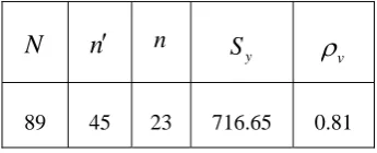
V. NUMERICAL ILLUSTRATION

[image:4.595.317.538.64.231.2]

To have a rough idea about the gain in efficiency of the proposed estimator (

s

_hgd2 ) over the Regression-type estimator

 

s

_lrd2 in double sampling, we take the empirical population considered in the literature (Source: Sukhatme & Sukhatme, 1970, p-256). The values of the population parameters obtained are given in Table 1. The mean square error and relative efficiency of the proposed estimator (

s

_hgd2 ) w.r.t. Regression-type estimator

 

s

_lrd2 and sample variance (

s

2_y) are given for some different values of



in the table 2. [image:4.595.64.237.288.358.2]

Table 1: Value of Population Parameters

Table 2: Mean Square Errors and Relative Efficiency

Proposed Estimator Vs. Regression-type Estimator and

Sample variance

-2 -1 0 1 2 3

40 60 80 100 120 140 160 180 200

_

Ef

ficie

n

cy



Regression Estimator

Sample variance

Proposed Estimator

Figure 1: Comparison of Proposed estimator with Regression-type estimator and sample variance

VI. CONCLUSION

From table 2, we can see that there is a significant gain in efficiency of the proposed estimator (

s

_hgd2 ) over the Regression-type estimator

 

s

_lrd2 in double sampling for

0

 



2

and sample variance (

s

2_y) for

2 2

1

_v

1

_v







  



. From the graph we also

see that for

0

 



2

, the efficiency of proposed estimator is more than the regression-type estimator and it is also more efficient than sample variance for wider range of



at moderate value of correlation coefficient. Hence we conclude that proposed estimator will always be better than the existing regression-type estimator under double sampling for

0

 



2

_{and sample variance for}

2 2

1

_v

1

_v







  



.

ACKNOWLEDGEMENT

Authors are thankful to the Referees for their valuable suggestions in improving the paper.

N

n



n

S

_y



_v

89 45 23 716.65 0.81



 

2

y

M S E s

 

2

lrd

MSE s

 

2

hgd

MSE s Efficiency

2

y

s

_lrd2

s

_hgd2

0 83539.758 56329.12 56329.12 100 148.30 148.30 0.5 83539.758 56329.12 46105.85 100 148.30 181.19

1 83539.758 56329.12 42698.09 100 148.30 195.65 1.5 83539.758 56329.12 46105.85 100 148.30 181.19

2 83539.758 56329.12 56329.12 100 148.30 148.30

IAENG International Journal of Applied Mathematics, 41:4, IJAM_41_4_01

(5)

REFERENCES

[1] S.N. Nath, “On Product Moments from a Finite Universe”, Journal of

the American Statistical Association, 63(322), 535-541, 1968.

[2] S.N. Nath, “More Results on Product Moments from a Finite Universe”, Journal of the American Statistical Association, 64(327), 864-869, 1969.

[3] A.K. Das and B. Tripathi, “Use of auxiliary information in estimating the finite population variance”, Sankhya, C 40, 139–148, 1978. [4] H.S. Jhajj and S.K. Srivastava, “A class of estimators using auxiliary

information for estimating finite population variance”, Sankhya, C

42(1–2), 87–96, 1980.

[5] M.S. Ahmed, A.D. Walid and A.O.H. Ahmed, “Some estimators for finite population variance under two-phase sampling”, Statistics in

Transition, 6(1), 143–150, 2003.

[6] H.S. Jhajj, M.K. Sharma and L.K. Grover, “An Efficient class of chain estimators of population variance under sub-sampling scheme”, Jour

Japan Statistical Society, 35(2), 273–286, 2005.

[7] C. Kadilar and H. Cingi, “Ratio estimators for the population variance in simple and stratified random sampling”, Applied Mathematics and

Computation, 173, 1047–1059, 2006.

[8] R. Fernandez-Alcala, J. Navarro-Moreno, J. C. Ruiz-Molina and A. Oya, “LMMSE Estimation based on Counting Observations”, IAENG Int. J. Appl. Math, 37:2, 2007.

[9] B.K. Pradhan, “Regression Type Estimators of Finite Population Variance Under Multiphase Sampling”, Bull. Malays. Math. Sci. Soc.,

(2) 33(2), 345–353, 2010.

[10] S.A. Al-hadhrami, “Estimation of the population variance using Ranked set sampling with auxiliary variable”, Int. J. Contemp. Math.

Sciences, Vol. 5, no.52, 2567-2576, 2010.

[11] H.P. Singh, R. Tailor, S. Singh and Jong-Min Kim, “Estimation of

population variance in successive sampling”, Qual. Quant, 45:477–

494, 2011.

APPENDIX

Appendix: I. For getting the expected value of

 

1 1, we

proceed as





2 2

1 1 2

1

2

1

y x

x y

s

E

S

 

















































₂

1

₂



_x2 _x2



_y2 _y2



x y

E

s

S

s

S

S S



















2 2

,

x y

Cov s

s

S S

 



(1)

On the similar line, other results involved in (2.1) can be derived.

II. Under Simple Random Sampling, covariance between sample variance of

x

and

y

can be obtained as











2 2 2 2 2 2

,

x y x x y y

Cov s s



E





s



S

s



S





E s s

 

2 2_x _y S S_x2 2_y





2





2 2 2

1 1

n n

i i x y

i i

E x x y y S S

n  n 

  

 __  _  __

 

  







 



 





 



2 2 2 2 _{2 2}

2

1 1

n n

i i x y

i i

E x X n x X y Y n y Y S S

n  

  

 __    _    __

 















 





 





 



2 2 2 2

2

1 1 1

2 2 ₂ 2 2 ₂ ₂

1 1

1

n n n

i i i

n

i x y

i

E x X y Y n x X y Y

n

n y Y x X n x X y Y S S

  





      

 



      





(2) The following results can be obtained by usual procedure





















2 2

1 1

2 2 20 02

1

1 1

n n

i i

E x X y Y

N n n n N n

N  N  

 

 _ _ 

 

 

 

 

 



(3)



 





















2 2

1

22 20 02

2 1

1 2 1 2

n

i i

E x X y Y

N n N n N N n n

N N n n N N  



 _ _ 

 

 

   

 

   



(4)



 





















2 2

1

22 20 02

2 1

1 2 1 2

n i i

E y Y x X

N n N n N N n n

N N n



n N N

 



 _ _ 

 

 

   

 

   



(5)



 







































2 2

22 3

20 02 3

2 11 3

6 1 6

1 2 3

1 1

1 2 3

2 1 1

1 2 3

N n N n N n

E x X y Y

N N N n

N N n N n n

N N N n

N N n N n n

N N N n



 



 

 _    _

 _ _ _

 

    

   



  

   



  

(6) Using the results of (3), (4), (5) and (6) in (2), and retaining terms up to first order of approximation, we have









2 2 2 2

22

1

,

1

x y x y

Cov s s

S S

n







On the similar line, other results involved in (3.8) can be derived.

IAENG International Journal of Applied Mathematics, 41:4, IJAM_41_4_01