https://doi.org/10.5194/amt-10-2093-2017 © Author(s) 2017. This work is distributed under the Creative Commons Attribution 3.0 License.
Remote sensing of PM2.5 during cloudy and nighttime periods
using ceilometer backscatter
Siwei Li1, Everette Joseph2, Qilong Min2, Bangsheng Yin2, Ricardo Sakai1, and Megan K. Payne1 1NOAA Center for Atmospheric Sciences, Howard University, Washington, DC 20001, USA
2Atmospheric Sciences Research Center, State University of New York at Albany, Albany, NY 12203, USA Correspondence to:Siwei Li ([email protected])
Received: 17 September 2016 – Discussion started: 29 November 2016 Revised: 8 May 2017 – Accepted: 8 May 2017 – Published: 8 June 2017
Abstract. Monitoring PM2.5 (particulate matter with aero-dynamic diameter d≤2.5 µm) mass concentration has be-come of more importance recently because of the nega-tive impacts of fine particles on human health. However, monitoring PM2.5 during cloudy and nighttime periods is difficult since nearly all the passive instruments used for aerosol remote sensing are not able to measure aerosol opti-cal depth (AOD) under either cloudy or nighttime conditions. In this study, an empirical model based on the regression be-tween PM2.5 and the near-surface backscatter measured by ceilometers was developed and tested using 6 years of data (2006 to 2011) from the Howard University Beltsville Cam-pus (HUBC) site. The empirical model can explain ∼56,
∼34 and ∼42 % of the variability in the hourly average PM2.5 during daytime clear, daytime cloudy and nighttime periods, respectively. Meteorological conditions and seasons were found to influence the relationship between PM2.5 mass concentration and the surface backscatter. Overall the model can explain∼48 % of the variability in the hourly av-erage PM2.5 at the HUBC site when considering the sea-sonal variation. The model also was tested using 4 years of data (2012 to 2015) from the Atmospheric Radiation Mea-surement (ARM) Southern Great Plains (SGP) site, which was geographically and climatologically different from the HUBC site. The results show that the empirical model can explain ∼66 and∼82 % of the variability in the daily av-erage PM2.5 at the ARM SGP site and HUBC site, respec-tively. The findings of this study illustrate the strong need for ceilometer data in air quality monitoring under cloudy and nighttime conditions. Since ceilometers are used broadly over the world, they may provide an important supplemental
source of information of aerosols to determine surface PM2.5 concentrations.
1 Introduction
The adverse impacts of high PM2.5 (particulate matter with aerodynamic diameter d≤2.5 µm) mass concentration on human health have been found from epidemiological stud-ies around the world (Samet et al., 2000; Pope et al., 2009; Krewski et al., 2009). PM2.5 concentration has been found to be associated with cardiopulmonary disease, lung cancer, and an increased morbidity and mortality (Schwartz et al., 1996; Gent et al., 2003, 2009; Dominici et al., 2006; Bell et al., 2007; Franklin et al., 2007; Slama et al., 2007; Pope et al., 2002; Miller et al., 2007; Lepeule et al., 2012). As an of-ficial norm to stand for fine-particle abundance, PM2.5 mass concentrations are monitored widely by the US Environmen-tal Protection Agency (EPA) through in situ instruments at surface monitoring sites. However, the number of EPA mon-itoring sites is limited. Therefore, remote sensing of PM2.5 from ground stations and satellites is desirable, allowing for fuller coverage of PM2.5 concentration between the EPA sur-face sites.
instruments like advanced lidars have the capacity to pro-vide the vertical distribution of aerosol backscatter coeffi-cient even under cloudy conditions or at nighttime. How-ever advanced lidar networks are rare due to the complexity and cost. Instead, ceilometers which are simple, automati-cally operating single-wavelength lidars are used broadly all over the world. Ceilometers were originally developed for cloud-based height retrieval. With the improvement of ac-curacy and power, the potential capabilities of ceilometers to detect mixing layer height and aerosol optical properties have been explored recently (Münkel et al., 2007; Markowicz et al., 2008; Heese et al., 2010; Tsaknakis et al., 2011; Wieg-ner and Geiß, 2012). Another distinct advantage of ceilome-ters is their small overlap distance, which makes them suit-able to detect aerosol information near the surface. PM2.5 concentration is an index of fine-particle mass concentration near the surface, while AOD is the integration of aerosol ex-tinction in the total atmospheric column. So using aerosol backscatter near the surface has an inherent advantage in the remote sensing of PM2.5 concentration.
There are extensive studies investigating the PM2.5–AOD relationship by the use of either an empirical statistical method (Engel-Cox et al., 2004; Liu et al., 2005, 2009; Gupta et al., 2006; Koelemeijer et al., 2006; Gupta and Christopher, 2008; Paciorek et al., 2008; Di Nicolantonio et al., 2009; Schaap et al., 2009; Lee et al., 2012; Sorek-Hamer et al., 2013; Strawa et al., 2013; Chudnovsky et al., 2014; Hu et al., 2013, 2014; Ma et al., 2014) or a chemical transportation model (Liu et al., 2004; Van Donkelaar et al., 2006, 2010; Kessner et al., 2013; Xu et al., 2015). In these studies, aerosol vertical distributions are estimated based on model simula-tion or under an assumpsimula-tion that aerosols are well mixed within the boundary layer and then decrease exponentially with height. Recently Li et al. (2016) developed an algo-rithm combining the backscatter measured from ceilometers with AOD for the PM2.5 retrieval. That work showed the ca-pability of the ceilometer to improve PM2.5 estimation by introducing measurements of aerosol optical properties near the surface. Although there are a plenty of studies on PM2.5 estimation, studies on the remote sensing of PM2.5 during ei-ther cloudy or nighttime periods are rare due to the limitation of measurements of AOD.
In this study, to estimate PM2.5 under cloudy or during night periods, we developed a regression model based on the relationship between PM2.5 and the ceilometer backscat-ter under different meteorological conditions. The model is tested and validated against the 6 years (2006–2011) of ground-based observations of ceilometer backscatter, PM2.5, AOD and meteorological conditions at the Howard Univer-sity Beltsville Campus (HUBC) site and the 4 years (2012– 2015) of data from the Atmospheric Radiation Measure-ment (ARM) Southern Great Plains (SGP) site. The data and model are described in Sect. 2. The results of the testing and evaluation of the model are illustrated in Sect. 3. The discus-sion is given in the last section.
2 Data and model 2.1 Data
In this study, the data were obtained from the HUBC site in Beltsville, MD, which is situated in a rural–suburban tran-sition region between Washington, DC and Baltimore, MD urban centers. The site has a wide range of collocated in-struments to observe atmospheric radiation, aerosol, cloud properties, meteorological conditions and air quality (Li et al., 2016), which makes the HUBC site suitable for PM2.5 investigations.
below 150 m among the 3 years is found within 10 % for the CT25k ceilometer.
The near-surface meteorological conditions – including temperature (T), relative humidity (RH), pressure, wind speed (W) and wind direction – are provided by a nearby 31 m micrometeorological tower, and the AOD observations and cloud optical depth (COD) are retrieved from a Multifil-ter Rotating Shadowband RadiomeMultifil-ter (MFRSR). The details of the MFRSR and the corresponding retrieval algorithms are introduced in Harrison et al. (1994), Harrison and Michal-sky (1994) and Min and Harrison (1996). The hourly aver-age PM2.5 are measured by a Met One BAM 1020 (beta ray attenuation monitor) from the collocated Maryland Depart-ment of the EnvironDepart-ment (MDE) monitor station (Li et al., 2016).
In this study, hourly average data were used for all the data sets. Precipitation and fog cases were screened out by using cloud effective radius larger than 15 µm, microwave-radiometer-measured liquid water path larger than 200 g m−2, ceilometer-derived cloud layer lower than 200 m and relative humidity larger than 95 %.
2.2 Model
For a ceilometer, the energy observed is a function of backscattering coefficient
P (x)=P0AηO (x) C1t
2x2 β (x) T
2(x) , (1)
whereP (x)andP0are the received and emitted powers from a ceilometer;Aandηare the area of the receiver and its effi-ciency, respectively; andxis the range from receiver to scat-tering volume.O (x)is overlap function,Cis light speed,1t
is the laser pulse duration andT (x)is the transmittance of the atmosphere between receiver and scattering volume.β (x)is the backscattering coefficient, which can be separated into two components:
β (x)=βm(x)+βa(x) . (2)
where βm(x) and βa(x) denote the backscattering by molecules and aerosols, respectively. The aerosol backscat-tering can be derived from the total backscatbackscat-tering coeffi-cient as the molecule scattering is well modeled by Rayleigh scattering. For the backscattering at the near-infrared wave-length, the contribution from molecules can be disregarded due to the rapidly decreased Rayleigh scattering with wave-length, soβ (x)is taken as∼βa(x)in this study.
With the assumption that aerosol size distribution is bi-modal lognormal and aerosol particles are spherical, Li et al. (2016) illustrated that both the extinction and PM2.5 can be expressed in terms of particle volume concentration (cvi)
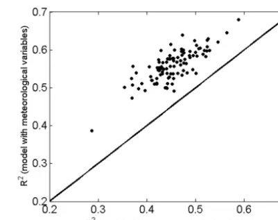
Figure 1.Comparison ofR2 out of the 100 independent cross-validations for the model without meteorological variables (Eq. 11) and the model with meteorological variables (Eq. 12) based on all the available daytime clear-sky cases at the HUBC site.
Table 1.Parameters based on the best fitting of 100 independent tests for Eq. (9).
Best-fitting parameters a0 a1 b1
Daytime clear −97.61 66.95 0.14
Daytime cloudy −100.00 94.02 0.05
Nighttime −100.00 85.70 0.08
for each mode as
ext(λ)=
2 X
i=1
cvih(Riσimλ), (3)
PM2.5=
2 X
i=1
cvig(Riσiρ), (4)
whereh(Riσimλ)andg(Riσiρ)are the integral functions of volume-concentration-normalized aerosol size distribution;
cis the total particle volume concentration; vi is the frac-tion of volume concentrafrac-tion for each mode i; Ri and σi are the geometric mean radius and the standard deviation of aerosol size distribution, respectively;λ is the wavelength;
mis the refractive index; andρ is the particle mass density. The relationship between the aerosol backscattering coeffi-cientβa(λ)and the extinction coefficient ext(λ)at the wave-lengthλis usually expressed by a lidar ratio (K):
K=ext(λ)
βa(λ). (5)
From Eqs. (3), (4) and (5) the relationship betweenβa(λ)
and PM2.5 can be expressed by
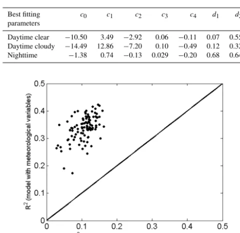
Table 2.Parameters based on the best fitting of 100 independent tests for Eq. (10).
Best fitting c0 c1 c2 c3 c4 d1 d2 parameters
Daytime clear −10.50 3.49 −2.92 0.06 −0.11 0.07 0.55 Daytime cloudy −14.49 12.86 −7.20 0.10 −0.49 0.12 0.32 Nighttime −1.38 0.74 −0.13 0.029 −0.20 0.68 0.64
Figure 2.Same as Fig. 1 but just for cases under daytime cloudy conditions.
where
F =K
2 P
i=1
vif (Ri, σi, m, λ)
2 P
i=1
vig(Ri, σi, ρ)
, (7)
The PM2.5 / backscatter ratioF only depends on aerosol size and composition. Given that the variation of aerosol size and composition could be associated with the meteorologi-cal conditions and the assumption that aerosols mixed well near the surface, an empirical model based on the relation-ship between PM2.5 and the backscatter near the surface is proposed as
PM2.5=a0+ a1+a2f (RH)+ n X
i=1
a2+iMi !
z Z
0
β (x, λ)dx
b2
+ε, (8)
where the hygroscopic grow factor is expressed as
f (RH)= 1
(1−RH)b1.
RH is relative humidity;M1throughMnare the meteorolog-ical factors including surface temperature, wind speed, wind direction and surface pressure;zis height;a0througha2+n,
Figure 3.Same as Fig. 1 but just for cases during nighttime periods.
b1 andb2are the regression coefficients; andε is the error term. In the following part, we will test the model perfor-mance without considering the meteorological variables. In that case, Eq. (8) can be expressed as
PM2.5=a0+a1
z Z
0
β (x, λ)dx
b1
+ε. (9)
When we test the model including the impacts from obser-vations of surfaceT, RH and W, Eq. (8) can be expressed as
PM2.5=c0+
c1+c2× 1
(1−RH)d1
+c3T+c4×W
z Z
0
β (x, λ)dx
d2
+ε. (10)
3 Results
Overfitting can occur when a regression model is too com-plex. The overfitted model describes random error or noise instead of the underlying relationship. To test and evaluate the model, cross-validations (CVs) are implemented on the 6 years of hourly average measurements at the HUBC site under the different conditions including daytime clear, day-time cloudy and nightday-time periods. For the cross-validation, we randomly select 90 % of the data as a training data set, use the remaining 10 % to test the models and repeat the pro-cedure 100 times to avoid random bias and misleadingR2
induced by overfitting. Cross-validations are conducted for each model under each condition.
Figure 4.The relationship between surface temperature and PM2.5 / backscatter ratio for(a)daytime clear-sky cases,(b)daytime cloudy cases and(c)nighttime cases.
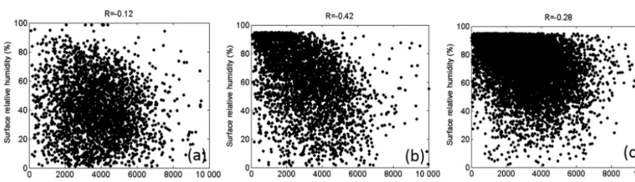
Figure 5.The relationship between surface relative humidity and PM2.5 / backscatter ratio for(a)daytime clear-sky cases,(b) daytime cloudy cases and(c)nighttime cases.
the average CV R2 out of the 100 times random cross-validations for the model (Eq. 10) is 0.56 (Fig. 1) with a root mean square error (RMSE) of 6.12 µg m−3. This re-sult is close to that of the nonlinear model which combines both AOD and the ceilometer backscattering (CVR2=0.60, RMSE=5.83 µg m−3)developed by Li et al. (2016) and per-formed much better than that of the model using AOD only (CVR2=0.40, RMSE=7.14 µg m−3; Li et al., 2016). With-out considering the meteorological conditions (Eq. 9), the av-erage CVR2 of the model is 0.45 (Fig. 2), which is better than that of the model using AOD only (Li et al., 2016) but not as good as the model including meteorological variables. Based on the fitted parameters (the parameters of the best fitting are shown in Tables 1, 2) from the 100 independent cross-validations (10 % of the total data), the average correla-tion coefficient between all the in situ measured PM2.5 under daytime clear-sky conditions and the simulated PM2.5 from the model without meteorological variables is 0.68 and in-creased to 0.76 when meteorological variables were included (Eq. 10).
Remote sensing of AOD is commonly based on the mea-surements of spectral extinction of solar radiation due to aerosol scattering and absorption in the atmospheric column from passive instruments. However most passive instruments
cannot readily discern AOD from COD under cloudy con-ditions. So any PM2.5 remote-sensing method relying on passive AOD measurements cannot retrieve PM2.5 under cloudy conditions. However, measurements of backscatter under cloudy conditions are still available for ceilometers, which can help to determine the near-surface aerosol extinc-tion when upper-layer clouds exist.
Under daytime cloudy conditions, the average CVR2 of the model without meteorological variables is only 0.11 (Fig. 2), which means only around 11 % of the variability in the hourly PM2.5 can be explained by the model. When meteorological factors are considered, the model can explain 34 % of the variability. Based on the fitted parameters of the 100 independent cross-validations, the average correla-tion coefficient between all the in situ measured PM2.5 un-der daytime cloudy conditions and the simulated PM2.5 from the model without meteorological variables is only 0.34, and it improved to 0.59 when meteorological variables were in-cluded in the model.
night-Figure 6.The relationship between surface wind speed and PM2.5 / backscatter ratio for(a)daytime clear-sky cases,(b)daytime cloudy cases and(c)nighttime cases.
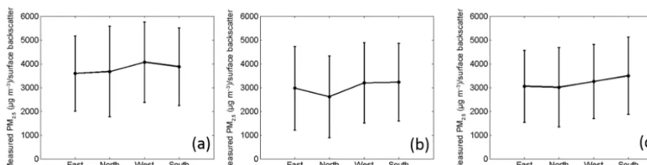
Figure 7.Average PM2.5 / backscatter ratio with standard deviation at four direction ranges – east (315 to 45◦), north (45 to 135◦), west (135 to 225◦) and south (225 to 315◦) – for(a)daytime clear cases,(b)daytime cloudy cases and(c)nighttime cases.
time periods, the average CVR2out of the 100 independent cross-validations for the model without meteorological vari-ables is 0.21, while the average CVR2 for the model with meteorological variables is 0.42 (Fig. 3). In this study, mea-surements under clear sky and cloudy sky were not separated during nighttime periods. Based on the fitted parameters of the 100 independent tests, the average correlation coefficient between all the in situ measured PM2.5 during nighttime and the simulated PM2.5 from the model without and with mete-orological variables was 0.47 and 0.65, respectively. 3.2 Impacts from meteorological variables
The previous results showed that without considering me-teorological factors the model predicting ability largely de-creased, especially under cloudy and nighttime conditions. Remote sensing of PM2.5 using backscattering coefficients is based on the relationship between PM2.5 and aerosol backscatter which is determined by aerosol physical and chemical properties. Aerosol physical and chemical charac-teristics are sensitive and dependent on meteorological con-ditions that can impact aerosol transportation, hygroscopic growth and aerosol nucleation/creation. Therefore, meteoro-logical conditions can be potentially used to estimate aerosol characteristics when the direct observations are not available. So taking into account the variations of meteorological
con-ditions may largely improve the model which is based on the regression between PM2.5 and backscattering coefficients.
To investigate impacts from different meteorological fac-tors on PM2.5 remote sensing, the relationship between each meteorological variable and the PM2.5 / backscatter ratio were analyzed in three data categories: daytime clear (AOD measurements are available), daytime cloudy and nighttime (Figs. 4–7). Among the meteorological variables, temper-ature was found to have the most prominent positive cor-relation with the PM2.5 / backscatter ratio. The corcor-relation coefficients are equal to 0.4, 0.46 and 0.29 under daytime clear, daytime cloudy and nighttime conditions, respectively (Fig. 4). In the eastern United States, sulfate dominates the aerosol chemical composition (Hand et al., 2012), and sul-fate concentrations are expected to increase with increasing temperature due to faster SO2oxidation. Fine particles have smaller backscatter coefficients due to the smaller size in-dex based on Mie theory (Wiscombe, 1980) than larger par-ticles with the same PM2.5 mass concentration. So at the HUBC site, the increase of temperature associated with the high PM2.5 / backscatter ratio could be due to the increase of fine particles.
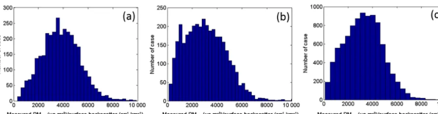
Figure 8.The number distribution of PM2.5 / backscatter ratio for(a)daytime clear cases,(b)daytime cloudy cases and(c)nighttime cases.
Table 3.Cross-validation tests of the model with different meteorological variables included.
Test R2 95 % confidence intervals
(RMSE) ofR2(of RMSE)
Test1: model including all available meteorological variables 0.43 (6.70) 0.421–0.429 (6.672–6.736)
Test2: model without surface temperature 0.37 (7.01) 0.367–0.375 (6.981–7.044)
Test3: model without relative humidity 0.39 (6.91) 0.385–0.393 (6.880–6.946)
Test4: model without wind speed 0.37 (7.01) 0.368–0.375 (6.978–7.043)
Test5: model without wind direction 0.42 (6.71) 0.420–0.428 (6.683–6.742)
Test6: model without surface pressure 0.42 (6.71) 0.421–0.429 (6.674–6.738)
Test7: model not including any meteorological variable 0.21 (7.88) 0.203–0.209 (7.846–7.914)
daytime clear, daytime cloudy and nighttime conditions, re-spectively (Fig. 5). Under high-relative-humidity conditions there can be significant variations in the aerosol optical prop-erties due to the aerosol hygroscopic growth effect. In the eastern United States, the dominant aerosols are composed of ammonium sulfate aerosols for which the ambient size will increase with the increase of the relative humidity due to hygroscopic growth. That can result in the decrease of the PM2.5 / backscatter ratio due to the increase of the aerosol extinction cross section while the aerosol dry mass is rela-tively invariant. It should be noted that the correlation coeffi-cient is−0.12 for the cases under daytime clear conditions, while it is −0.42 under daytime cloudy conditions. Chu et al. (2015) showed that the effect of hygroscopic growth on extinction is more prominent when the relative humidity is larger. Under nighttime conditions, including both the clear and cloudy situations, the correlation coefficient is−0.28.
A negative association is also found between the wind speed and PM2.5 / backscatter ratio under all the three con-ditions (Fig. 6). That may be explained by the associa-tion of higher PM2.5 concentraassocia-tions with more stagnant, weaker wind conditions (Tai et al., 2010). Based on the aver-age PM2.5 / backscatter ratio at four wind direction ranges – east (315 to 45◦), north (45 to 135◦), west (135 to 225◦)and south (225 to 315◦)– the variation of the mean PM2.5 / backscatter ratio at the four different wind directions was found to be small (within 10 %) compared to the stan-dard deviation (∼50 % of the mean value) at the HUBC site
(Fig. 7). The association of the surface pressure with the PM2.5 / backscatter ratio was found to be weak, with the cor-relation coefficient equal to−0.05 (not shown). The distribu-tions of PM2.5 / backscatter ratio under the three condidistribu-tions are shown in Fig. 8. Statistically, the PM2.5 / backscatter ra-tio under daytime clear-sky condira-tions is larger than that un-der daytime cloudy or nighttime conditions.
Figures 4–7 show the potential impacts of meteorologi-cal factors on model prediction. However, some information possibly overlaps among the different meteorological vari-ables. To investigate the contribution of each meteorological variable to improving the model predicting power, the model was tested with different meteorological variable combina-tions. For each test, the cross-validation was randomly re-peated 100 times based on all the available cases, including the daytime clear, daytime cloudy and nighttime periods.
Figure 9.Comparison of measured PM2.5 and modeled PM2.5 when meteorological variables are not taken into account.(a)The model is non-seasonally fitted, and(b)the model is seasonally fitted. The colors stand for the number density of the points.
Figure 10.Same as Fig. 9 but with all meteorological variables taken into account.
3.3 Seasonally fitting
Besides meteorological factors, the seasonal variations of aerosol physical and chemical properties could impact the PM2.5 / backscatter ratio and then PM2.5 retrievals. To in-vestigate the impacts of seasonal variations on PM2.5 re-trievals, we fit the model seasonally and compared that per-formance with the model fitted on all the data without con-sidering seasonal variation. Just as in the previous section, the cross-validations were implemented for each test. The parameters of the fitting with the median CVR2out of the 100 independent cross-validations for each fitting method are used to calculate the correlation between the in situ measure-ments of PM25 and the simulated PM2.5. When meteoro-logical variables were not considered, the simulated PM2.5 from the model with the seasonally fitted parameters had a much stronger association with the in situ measured PM2.5 (R=0.57) than the model with the non-seasonally fitted pa-rameters (R=0.45; Fig. 9). When meteorological variables were taken into account, the correlation coefficient between
the simulation and the in situ measurements of PM2.5 for the model with the seasonally fitted parameters and the model with the non-seasonally fitted parameters was 0.69 and 0.65, respectively (Fig. 10), and the average CVR2 was 0.48 and 0.43. The meteorological conditions have seasonal variation, so taking into account meteorological variables in the model can mitigate downside impacts of ignoring seasonal varia-tions of aerosol properties on PM2.5 prediction.
3.4 Test in a different region
Figure 11.Comparison of cross-validationR2of the model without meteorological variables and model with meteorological variables during daytime clear, daytime cloudy and nighttime periods with the data from ARM SGP site.
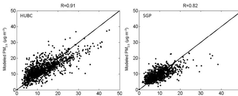
Figure 12.Comparison of daily average PM2.5 between in situ measurements and model simulation at the HUBC site and ARM SGP site.
The Vaisala CL31 has the same laser system, wavelength and measurement range as CT25k but improved spatial and tem-poral resolution and algorithms for cloud amount and mixing layer height detection (Münkel et al., 2007). To estimate the possible response changing of the CL31 ceilometer in dif-ferent years, we compared the same 3 years (2012, 2013, 2014) of yearly average ceilometer backscatter profiles un-der nighttime clear conditions as used for the CT25K. The largest difference of the yearly average backscatter under nighttime clear conditions among the 3 years (2012, 2013 and 2014) is found within 3 % for the backscatter below 150 m. The principle of the algorithm (Eqs. 1 to 10) is ap-plicable to most lidars with small overlap distance. So it is possible to use the model with the Vaisala CL31. In the test, we used 4 years (from 2012 to 2015) of measurements of Vaisala CL31 ceilometer backscatter and the surface meteo-rological conditions provided by the ARM SGP site and the FRM/FEM PM2.5 mass concentration from the nearest EPA site (36.697◦N and 97.081◦W; Air Quality System Data Mart, available via http://www.epa.gov/airdata). The same cross-validation procedure was implemented in the measure-ments at the ARM SGP site under daytime clear, daytime cloudy and nighttime periods. For the hourly average PM2.5,
4 Discussion
Remote sensing of PM2.5 is generally based on AOD mea-surements due to its strong relationship with PM2.5. For nearly all the passive instruments, the measurements of AOD rely on solar radiation. Ceilometers are compact, low-cost and unattended operational lidars and have been broadly used around the world. Although their laser power is relatively lower, the advantages of the small overlap distance and unat-tended and continuous operation make ceilometers suitable for remote sensing of aerosols near the surface. Moreover, the measurements of ceilometers do not rely on solar radia-tion, which makes them capable of retrieving aerosols during cloudy or nighttime periods.
In this study, an empirical model based on the regression between PM2.5 concentrations and ceilometer backscatter measurements was developed and tested with 6 years of ob-servations at the HUBC site. The empirical model can ex-plain∼56,∼34 and∼42 % of the variability in the hourly average PM2.5, respectively, during the daytime clear, day-time cloudy and nightday-time periods. During the dayday-time clear periods the prediction capability was close to that of the model combining AOD and backscatter (explain∼60 % of the variability) developed by Li et al. (2016), while during the daytime cloudy or nighttime period only the empirical model, which is independent of AOD, is available for the PM2.5 retrieval.
The impacts of meteorological conditions on the relation-ship between the in situ measured PM2.5 and the ceilometer-measured backscatter were analyzed. The prominent posi-tive relationship found between the surface temperature and the PM2.5 / backscatter ratio could be due to the faster SO2 oxidation under higher temperature given that the dominant aerosol chemical composition is sulfate in the eastern United States. The measured relative humidity showed a signifi-cant negative association with the PM2.5 / backscatter ra-tio, which could be due to hygroscopic growth of aerosols. The wind speed also showed a negative association with the PM2.5 / backscatter ratio, but the relationship between the measured wind direction and PM2.5 / backscatter ratio was found to not be obvious at the HUBC site. However, it is noteworthy that wind direction can be related to aerosol transportation and is usually associated with aerosol concen-tration and type. Although there was no significant associa-tion of the wind direcassocia-tion with the PM2.5 / backscatter ratio at the HUBC site, wind direction impacts could be signifi-cant at other places where transported aerosols like dust are found near the surface. Aerosol properties usually vary sea-sonally due to the seasea-sonally varied meteorological condi-tions, large-scale transportation and local emission of anthro-pogenic and natural aerosols. Taking into account the meteo-rological conditions in the model can to some extent mitigate the seasonal impacts on the PM2.5 retrieval, and conducting the seasonal fitting can further improve the model predicting capability. Overall, the model with the seasonally fitted
pa-rameters can explain∼48 % of the variability in the hourly PM2.5 including during daytime clear, daytime cloudy and nighttime periods at the HUBC site. Aerosol physical and chemical characteristics which are associated with aerosol dry mass and optical properties could vary at different loca-tions. So a test was implemented based on the observations from the ARM SGP site, which is geographically and clima-tologically different from the HUBC site. The results show that the impacts of meteorological conditions on the retrieval of PM2.5 using the ceilometer backscatter at the ARM SGP site are not as prominent as those at the HUBC site. That could be due to the different aerosol types in the SGP area and the DC area. In addition, the model parameters could be different for different aerosol types or in different climatic regions. That is because the relationship between PM2.5 and aerosol backscatter is related to aerosol types and sizes (Li et al., 2016), and the relationship between meteorological con-ditions and aerosols (i.e. size, composition) could vary with variation of aerosol types or climatic regions. Overall, the regression model using the ceilometer backscatter with me-teorological variables could explain around 66 and 82 % of the variability in the daily average PM2.5 at the ARM SGP site and the HUBC site, respectively. It is worth noting that both the instrument hardware-related background signals and software-related artifacts could impact attenuated backscter profiles observed by ceilomebackscters. Further processing of at-tenuated backscatter profiles is needed to get accurate atten-uated backscatter observations from ceilometers especially under low signal-to-noise ratio situations (Kotthaus et al., 2016). In this study, we only use the attenuated backscatter at low altitude, where both the Vaisala CT25k and CL31 have high signal-to-noise ratio for lidar return signals and hourly average will also decrease noise. So the potential background signals and systematic artifacts should have small impacts on the regression model performance. However, the parameters of the regression model could be different for different in-struments.
The most important objectives of this study were to develop an algorithm for remote sensing PM2.5 during cloudy and nighttime periods by using ceilometer-measured backscatter. Retrievals of PM2.5 during cloudy or nighttime periods are very rare based on current remote-sensing meth-ods. A large number of ceilometers have been used over the world, especially in the Europe and United States. The ex-ploitation of the ceilometer on PM2.5 remote sensing could provide important information for air quality purpose, espe-cially in helping to improve PM2.5 forecast over a larger area and can help fill the gaps among the EPA stations. Moreover that will largely increase the monitoring of air quality during cloudy or/and nighttime periods.
Competing interests. The authors declare that they have no conflict of interest.
Acknowledgements. This work was supported by the National Oceanic and Atmospheric Administration, Educational Partner-ship Program, US Department of Commerce, under agreement no. NA11SEC4810003, and supported by the National Aero-nautics and Space Administration grant nos. NNX08BA42A and NNX10AQ11A.
Edited by: P. Stammes
Reviewed by: W. Thomas and R. Koelemeijer
References
Bell, M. L., Ebisu, K., and Belanger, K.: Ambient air pollution and low birth weight in Connecticut and Massachusetts, Environ. Health Persp., 115, 1118–1124, 2007.
Chu, D. A., Ferrare, R., Szykman, J., Lewis, J., Scarino, A., Hains, J., Burton, S., Chen, G., Tsai, T., Hostetler, C., Hair, J., Holben, B., and Crawford, J.: Regional characteristics of the relationship between columnar AOD and surface PM2.5: Application of lidar aerosol extinction profiles over BaltimoreeWashington Corridor during DISCOVER-AQ, Atmos. Environ., 101, 338–349, 2015. Chudnovsky, A., Lyapustin, A., Wang, Y., Tang, C., Schwartz, J.,
and Koutrakis, P.: High resolution aerosol data from MODIS satellite for urban air quality studies, Cent. Eur. J. Geosci., 6, 17–26, https://doi.org/10.2478/s13533-012-0145-4, 2014. Di Nicolantonio, W., Cacciari, A., and Tomasi, C.: Particulate
mat-ter at surface, Northern Italy monitoring based on satellite remote sensing, meteorological fields, and in-situ samplings, IEEE J. Se-lected Topics Appl. Earth Observ. Remote. Sens., 2, 284–292, 2009.
Dominici, F., Peng, R. D., Bell, M. L., Pham, L., McDermott, A., Zeger, S. L., and Samet, J. M.: Fine particulate air pollution and hospital admission for cardiovascular and respiratory diseases, JAMA, 295, 1127–1134, 2006.
Engel-Cox, J. A., Holloman, C. H., Coutant, B. W., and Hoff, R. M.: Qualitative and quantitative evaluation of MODIS satellite sensor data for regional and urban scale air quality, Atmos. Environ., 38, 2495–2509, 2004.
Franklin, M., Zeka, A., and Schwartz, J.: Association between PM2.5 and all-cause and specific-cause mortality in 27 US com-munities, J. Expo. Sci. Environ. Epidemiol., 17, 279–287, 2007. Gent, J. F., Triche, E. W., Holford, T. R., Belanger, K., Bracken, M. B., Beckett, W. S., and Leaderer, B. P.: Association of low-level ozone and fine particles with respiratory symptoms in children with asthma, JAMA, 290, 1859–1867, 2003.
Gent, J. F., Koutrakis, P., Belanger, K., Triche, E., Holford, T. R., Bracken, M. B., and Leaderer, B. P.: Symptoms and medication use in children with asthma and traffic-related sources of fine particle pollution, Environ. Health Persp., 117, 1168–1174, 2009. Gupta, P. and Christopher, S. A.: Seven year particulate matter air quality assessment from surface and satellite measurements, At-mos. Chem. Phys., 8, 3311–3324, https://doi.org/10.5194/acp-8-3311-2008, 2008.
Gupta, P., Christopher, S. A., Wang, J., Gehrig, R., Lee, Y., and Kumar, N.: Satellite remote sensing of particulate matter and air quality assessment over global cities, Atmos. Environ., 40, 5880– 5892, 2006.
Hand, J. L., Schichtel, B. A., Malm, W. C., and Pitchford, M. L.: Particulate sulfate ion concentration and SO2emission trends in
the United States from the early 1990s through 2010, Atmos. Chem. Phys., 12, 10353–10365, https://doi.org/10.5194/acp-12-10353-2012, 2012.
Harrison, L. and Michalsky, J.: Objective algorithms for the retrieval of optical depths from ground-based measurements, Appl. Opt., 33, 335126–335132, 1994.
Harrison, L., Michalsky, J., and Berndt, J.: Automated multifilter ro-tating shadow-band radiometer: An instrument for optical depth and radiation measurements, Appl. Opt., 33, 5118–5125, 1994. Heese, B., Flentje, H., Althausen, D., Ansmann, A., and Frey,
S.: Ceilometer lidar comparison: backscatter coefficient retrieval and signal-to-noise ratio determination, Atmos. Meas. Tech., 3, 1763–1770, https://doi.org/10.5194/amt-3-1763-2010, 2010. Hu, X., Lance, W., Al-Hamdan, M., Crosson, W., Estes Jr, M., Estes,
S., Quattrochi, D., Sarnat, J., and Liu, Y.: Estimating Ground-level PM2.5 concentrations in the Southeastern U.S. using Ge-ographically Weighted Regression, Environ. Res., 121, 1–10, 2013.
Hu, X., Lance, W., Lyapustin, A., Wang, Y., Al-Hamdan, M., Crosson, W., Estes Jr, M., Estes, S., Quattrochi, D., Puttaswamy, S., and Liu, Y.: Estimating Ground-level PM2.5 Concentrations in the Southeastern U.S. using MAIAC AOD Retrievals and a Two-Stage Model, Remote Sens. Environ., 140, 220-232, 2014. Kessner, A., Wang, J., Levy, R., and Colarco, P.: Remote
sensing of surface visibility from space: a look at the United States East Coast, Atmos. Environ., 81, 136e147, https://doi.org/10.1016/j.atmosenv.2013.08.050, 2013.
Koelemeijer, R. B. A., Homan, C. D., and Matthijsen, J.: Compari-son of spatial and temporal variations of aerosol optical thickness and particulate matter over Europe, Atmos. Environ., 40, 5304– 5315, 2006.
Kotthaus, S., O’Connor, E., Münkel, C., Charlton-Perez, C., Haef-felin, M., Gabey, A. M., and Grimmond, C. S. B.: Recommenda-tions for processing atmospheric attenuated backscatter profiles from Vaisala CL31 ceilometers, Atmos. Meas. Tech., 9, 3769– 3791, https://doi.org/10.5194/amt-9-3769-2016, 2016.
Krewski, D., Jerrett, M., Burnett, R. T., Ma, R., Hughes, E., Shi, Y., Turner, M. C., Pope, C. A., Thurston, G., Calle, E. E., and Thun, M. J.: Extended follow-up and spatial analysis of the American Cancer Society study linking particulate air pollution and mor-tality, Health Effects Inst. Research., 2009.
Lee, H. J., Coull, B. A., Bell, M. L., and Koutrakis, P.: Use of satellite-based aerosol optical depth and spatial clustering to pre-dict ambient PM2.5 concentrations, Environ Res., 118, 8–15, https://doi.org/10.1016/j.envres.2012.06.011, 2012.
Lepeule, J., Laden, F., Dockery, D., and Schwartz, J.: Chronic ex-posure to fine particles and mortality: an extended follow up of the Harvard six cities study from 1974 to 2009, Environ. Health Persp., 120, 965–970, https://doi.org/10.1289/ehp.1104660, 2012.
Li, S., Joseph, E., and Min, Q.: Remote sensing of
backscat-tering profile, Remote Sens. Environ., 183, 120–128, https://doi.org/10.1016/j.rse.2016.05.025, 2016.
Liu, Y., Park, R. J., Jacob, D. J., Li, Q. B., Kilaru, V., and Sar-nat, J. A.: Mapping annual mean ground-level PM2.5 concentra-tions using Multiangle Imaging Spectroradiometer aerosol opti-cal thickness over the contiguous United States, J. Geophys. Res., 109, D22206, https://doi.org/10.1029/2004JD005025, 2004. Liu, Y., Sarnat, J. A., Kilaru, V., Jacob, D. J., and Koutrakis, P.:
Es-timating Ground-Level PM2.5 in the Eastern United States Us-ing Satellite Remote SensUs-ing, Environ. Sci. Technol., 39, 3269– 3278, https://doi.org/10.1021/es049352m, 2005.
Liu, Y., Paciorek, C. J., and Koutrakis, P.: Estimating Regional Spatial and Temporal Variability of PM Concentrations Using Satellite Data, Meteorology, and Land Use Information, Environ. Health Persp., 117, 886–892, 2009.
Ma, Z., Hu, X., Huang, L., Bi, J., and Liu, Y.:
Es-timating Ground-Level PM2.5 in China Using Satellite Remote Sensing, Environ. Sci. Technol., 48, 7436–7444, https://doi.org/10.1021/es5009399, 2014.
Markowicz, K. M., Flatau, P. J., Kardas, A. E., Remiszewska,
J., Stelmaszczyk, K., and Woeste, L.: Ceilometer
Re-trieval of the Boundary Layer Vertical Aerosol Extinc-tion Structure, J. Atmos. Ocean. Technol., 25, 928–944, https://doi.org/10.1175/2007JTECHA1016.1, 2008.
Miller, K., Siscovick, D., Sheppard, L., Shepherd, K., Sullivan, J., Anderson, G., and Kaufman, J.: Long-term exposure to air pol-lution and incidence of cardiovascular events in women, New England Journal of Medicine, 356, 447–458, 2007.
Min, Q. and Harrison, L.: Cloud properties derived from surface MFRSR measurements and comparison with GOES results at the ARM SGP site, Geophys. Res. Lett., 23, 1641–1644, 1996. Münkel, C., Eresmaa, N., Räsänen, J., and Karppinen, A.:
Retrieval of mixing height and dust concentration with
lidar ceilometer, Bound.-Lay. Meteorol., 124, 117–128,
https://doi.org/10.1007/s10546-006-9103-3, 2007.
Paciorek, C. J., Liu, Y., Moreno-Macias, H., and Kondragunta, S.: Spatiotemporal Associations between GOES Aerosol Optical Depth Retrievals and Ground-Level PM2.5, Environ. Sci. Tech-nol., 42, 5800–5806, https://doi.org/10.1021/es703181j, 2008. Pope, C. A., Burnett, R. T., Thun, M. J., Calle, E. E., Krewski,
D., Ito, K., and Thurston, G. D.: Lung cancer, cardiopulmonary mortality, and long-term exposure to fine particulate pollution. JAMA: the Journal of the American Medical Association, 287, 1132–1141, 2002.
Pope, C. A., Ezzati, M., and Dockery, D. W.: Fine-particulate air pollution and life expectancy in the United States, N England J Med., 360, 376–386, https://doi.org/10.1056/NEJMsa0805646, 2009.
Samet, J. M., Dominici, F., Curriero, F. C., Coursac, I., and Zeger, S. L.: Fine particulate air pollution and mortality in 20 U.S. cities, 1987–1994, N. Engl. J. Med., 343, 1742–1749, https://doi.org/10.1056/NEJM200012143432401, 2000. Schaap, M., Apituley, A., Timmermans, R. M. A., Koelemeijer,
R. B. A., and de Leeuw, G.: Exploring the relation between
aerosol optical depth and PM2.5 at Cabauw, the Netherlands,
Atmos. Chem. Phys., 9, 909–925, https://doi.org/10.5194/acp-9-909-2009, 2009.
Schwartz, J., Dockery, D. W., and Neas, L. M.: Is daily mortality associated specifically with fine particles?, J. Air Waste Manag. Assoc., 46, 927–939, 1996.
Slama, R., Morgenstern, V., Cyrys, J., Zutavern, A., Herbarth, O., Wichmann, H. E., and Heinrich, J.: Traffic-related atmospheric pollutants levels during pregnancy and offspring’s term birth weight, A study relying on a land-use regression exposure model, Environ. Health Persp., 115, 1283–1292, 2007.
Sorek-Hamer, M., Strawa, W. A., Chatfield, B. R.,
Es-swein, R., Cohen, A., and Broday, M. D.: Improved
retrieval of PM2.5 from satellite data products using
non-linear methods, Environ. Pollut., 182, 417–423,
https://doi.org/10.1016/j.envpol.2013.08.002, 2013.
Strawa, A. W., Chatfield, R. B., Legg, M., Scarnato, B.,
and Esswein, R.: Improving Retrievals of Regional
PM2.5 Concentrations From MODIS and OMI
Multi-Satellite Observations, J. Air Waste Manage. Assoc., 63, https://doi.org/10.1080/10962247.2013.822838, 2013.
Tai, P. K. A., Mickley, L. J., and Jacob, D. J.: Correlations be-tween fine particulate matter (PM2.5) and meteorological vari-ables in the United States: Implications for the sensitivity of PM2.5 to climate change, Atmos. Environ., 44, 3976–3984, https://doi.org/10.1016/j.atmosenv.2010.06.060, 2010.
Tsaknakis, G., Papayannis, A., Kokkalis, P., Amiridis, V., Kam-bezidis, H. D., Mamouri, R. E., Georgoussis, G., and Avdikos, G.: Inter-comparison of lidar and ceilometer retrievals for aerosol and Planetary Boundary Layer profiling over Athens, Greece, At-mos. Meas. Tech., 4, 1261–1273, https://doi.org/10.5194/amt-4-1261-2011, 2011.
van Donkelaar, A., Martin, R. V., and Park, R. J.: Estimating ground-level PM2.5 using aerosol optical depth determined from satellite remote sensing, J. Geophys. Res., 111, D21201, https://doi.org/10.1029/2005JD006996, 2006.
van Donkelaar, A., Martin, R. V., Brauer, M., Kahn, R., Levy, R., Verduzco, C., and Villeneuve, P. J.: Global estimates of am-bient fine particulate matter concentrations from satellite-based aerosol optical depth: Development and application, Environ. Health Persp., 118, 847–855, 2010.
Wiegner, M. and Geiß, A.L Aerosol profiling with the Jenop-tik ceilometer CHM15kx, Atmos. Meas. Tech., 5, 1953–1964, https://doi.org/10.5194/amt-5-1953-2012, 2012.
Wiegner, M. and Gasteiger, J.: Correction of water vapor absorption for aerosol remote sensing with ceilometers, Atmos. Meas. Tech., 8, 3971–3984, https://doi.org/10.5194/amt-8-3971-2015, 2015. Wiegner, M., Madonna, F., Binietoglou, I., Forkel, R., Gasteiger, J.,
Geiß, A., Pappalardo, G., Schäfer, K., and Thomas, W.: What is the benefit of ceilometers for aerosol remote sensing? An answer from EARLINET, Atmos. Meas. Tech., 7, 1979–1997, https://doi.org/10.5194/amt-7-1979-2014, 2014.
Wiscombe, W.: Improved mie scattering algorithms, Appl. Opt., 19, 1505–1509, 1980.
Xu, J.-W., Martin, R. V., van Donkelaar, A., Kim, J., Choi, M., Zhang, Q., Geng, G., Liu, Y., Ma, Z., Huang, L., Wang, Y., Chen, H., Che, H., Lin, P., and Lin, N.: Estimating ground-level PM2.5