Placement of Renewable Distributed Generation Using Harmony Search Optimization Technique

Placement of Renewable Distributed

Generation Using Harmony Search

Optimization Technique

E.Aswini1, M.Seshu2

P.G Student, EEE Department, Prasad V.Potluri Siddhartha Institute of Technology, Vijayawada, Andhra Pradesh, India1

Assistant Professor, EEE Department, Prasad V.Potluri Siddhartha Institute of Technology, Vijayawada, Andhra Pradesh India2

ABSTRACT: In this paper a new approach using Harmony Search (HS) algorithm is presented for placing Distributed Generators (DGs) in radial distribution systems. HS is used for multiple objective planning, to evaluate the DG placement and sizing by considering the power losses and voltage profile as objective functions. HS is operated on 12-bus, 15-bus and 33-bus radial distribution system(RDS). Obtained results of 12-12-bus, 15-bus and further 33-bus in MATLAB are compared with other DG placement techniques such as Improved Analytical (IA), Mixed Integer Non Linear Programming (MINLP). The proposed method is found to be more effective in terms of voltage stability enhancement and power loss minimization.

KEYWORDS: Distributed generation, harmony search algorithm, multi-objective optimization, loss minimisation, improving voltage profile.

I. INTRODUCTION

Growing load demand within the distribution network provides scope for analyzing the distribution network to reach the demand with the current infrastructure. And the feasible energy development is an important concern, all over the world, for performing economical and industrial growth. Due to this there has been an excellent interest within the integration of distributed generation (DG) units at the distribution level. Advantages of DGs [1] depends on how they are placed in the power system, namely on their location and size. Distribution networks are characterized by the high R/X ratio causing a large voltage drop and substantial power losses in the power system. Studies have indicated that inappropriate selection in terms of both site and size of DG, may lead to greater system losses than the losses without DG.

The optimum DG allocation may be a complicated problem with nonlinear objective function and nonlinear constraints, during which heuristic algorithms are a descent selection for placing DGs. The optimization problem of single and multiple DG placements is done using GA [4], PSO [5, 6], ant colony [14], artificial bee colony [8], differential evolution [7], and harmony search [10], [11]. Although, the heuristic algorithms are derivative free and halfwit to implement, they have much iteration to ensure converged solution. Thus, they become computationally intensive. These techniques could give nearly optimum solutions.

market, however here thought about the Renewable Energy Sources.However the strategy confirmed during this paper are often effective and helpful to system designers in selecting proper sites to place DG.

II. MATHEMATICAL FORMULATION

The main objective of the proposed approach is to minimize the total system power loss by Optimal Sizing and sitting of Distributed Generation in radial distribution system by considering the constraints.

They are classified into 2 types: 1) Equality constraints

2) Inequality constraints

A. EQUALITY CONSTRAINTS: Real and Reactive power balance constraints are related to the non linear power flow equations, the power balance constraints is formulated as follows

i DGi Di

P



P



P

(1)

i DGi Di

Q



Q



Q

(2) Where

i

P

is real power flow at bus i in KW

i

Q

is reactive power flow at bus i in KVar

DGi

P

is real power generation from DG placed at bus i in KW

DGi

Q

is reactive power generation from DG placed at bus i in KVar

Di

P

is real power demand at bus i in KW

Di

Q

is reactive power demand at bus i in KVAR

B. INEQUALITY CONSTRAINTS: An inequality constraint lies between acceptable limits to satisfy the objective function.

a) Bus Voltage limits

Bus Voltage magnitude is to be kept within acceptable limits then the bus voltage limit is given by

min max

i i i

V



V



V

(3) Where

V

_imin and

V

_imax are lower and upper bound bus voltage limits in P.U

b) DG Capacities

The capacity of each DG unit should be differ around its nominal value. So that each DG unit must be maintained with in an acceptable limit.

The capacity of DG is given as follows

min max

DGi DGi DGi

P



P



P

(4)

min max

DGi DGi DGi

Q



Q



Q

(5) Where,

min DGi

P

and

P

_DGimax are minimum and maximum real power generation from DG capacity in KW.

min DGi

III. PROPOSED METHODOLOGY

In this section a various radial distribution system is used to locate the DG in an optimal place with the proper sizing. The Proposed Approach needs power flow to be run for two times, one for the initial base case and another at the final stage with the DG to obtain the optimal solution.

HARMONY SEARCH ALGORITHMS

An overview of the basic Harmony Search (HS) algorithm is presented in this section, followed by improved version of the HS algorithm reported in the literature, Improved Harmony Search (IHS).

A.HARMONY SEARCH (HS)

The HS is based on the natural musical process which searches for a perfect state of harmony. The HS algorithm does not require initial values for the decision variables and uses a stochastic random search. In general, the HS algorithm works as follows [10]:

Step1. Define the objective function and decision variables. Input the system parameters and the boundaries of the decision variables.

The optimization problem can be defined as Minimise f(x)

Subject to x_iLx_ix_iU (i=1, 2...N)

Where

x

_iL and

x

_iU are the lower and upper bounds for decision variables.

The HS algorithm parameters are specified in this step. They are the harmony memory size (HMS) or the number of solution vectors in harmony memory, the harmony memory considering rate (HMCR), the distance bandwidth (bw), the pitch adjusting rate (PAR), and the number of improvisations (K)or stopping criterion, where K is the same as the total number of function evaluations.

Ste 2. Initialize the harmony memory (HM). The harmony memory is a memory location where all the solution vectors (sets of decision variables) are stored. The initial harmony memory is randomly generated in the region

[

x

_iL,

x

_iU ] (i=1, 2...N). This is done based on the following equation:

() (

)

j

i iL iU iL

x



x



rand



x



x

(j=1, 2, HMS) (6) Where

rand

()

is a random number from a uniform distribution of [0, 1].

Step3. Improvise a new harmony from the harmony memory. Generating a new harmony

new

x

is called improvisation, which is based on 3 rules: memory consideration, pitch adjustment, and random selection.

First of all, a uniform random number r is generated in the range [0, 1]. If r is less than the HMCR, the decision variable

x

_inew is generated by the memory consideration; otherwise

x

_inew, is obtained by a random selection. Then, each decision variable

x

_inew will undergo a pitch adjustment with a probability of PAR if it is produced by the memory consideration. The pitch adjustment rule is given as follows:

x

_inew



x

_inew

 

r bw

(7)

Step5. Repeat Steps 3–4 until the stopping criterion (maximum number of improvisations, K) is met.

B.THE IMPROVED HARMONY SEARCH (IHS)

An improved harmony search algorithm (IHS) is proposed in [11], in which the key modifications are about PAR (Pitch adjustment Rate) and bw (Band width). In the HS, PAR, and bw are all constants, but the IHS updated them dynamically as follows

max min

min

( )

(

PAR

PAR

)

PAR k

PAR

k

K







(8)

min

max max

( )

exp

bw

In

bw

bw k

bw

k

K











































(9)

Where k is current number of improvisations, and K is maximum number of improvisations. Numerical results on engineering optimization problems reveal that the IHS can find better solutions compared to the HS. In IHS, the numbers of parameters are increased, which is not good, and this is the main drawback of the IHS. It should be noted that in order to get the optimum point by heuristic algorithms, the parameters of the algorithm must be tuned for the problem at hand.

Fig 1.Flow chart of Harmony Search

IV. SIMULATION RESULTS AND DISCUSSION

The Proposed formulation is tested on IEEE 12 bus, 15 bus and 33 bus distribution systems. And the results of 33 bus are then compared with the Improved Analytical (IA)and Mixed Integer Non-Linear Programming (MINLP), which are the promising ways for multiple DG placements.

Fig 2.Single line diagram of 12 bus RDN

Fig 3.Single line diagram of 15 bus RDN

Fig 4.Single line diagram of 33 bus RDS

delivering real and reactive power. However, projected formulation is generalized and may be enforced for any type of DGs. The power factor of DG unit provides real and reactive power, which are constrained between 0.8 and 1.0.The base case values for both 12-bus, 15 bus are 100MVA, 11 KV and for 33-bus base case values are 100MVA, 12.66KV.

The total real and reactive power demands in IEEE 12-bus system are 415KW and 403 MVar respectively. System line loss without DG is 20.286 KW. Similarly for IEEE 15 bus system total real and reactive power demands are 1.22MW, 1.25 MVar. System line loss without DG is of 59.4KW.

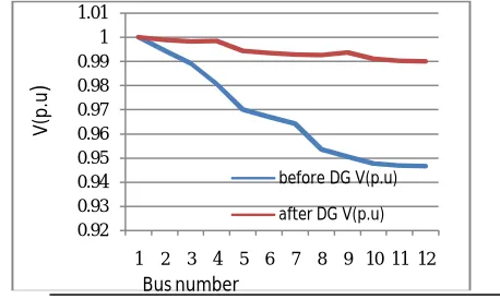
Fig 5 V (p.u) waveform of 12 bus before and after DG placement

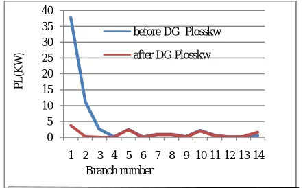
Fig6. PL (KW) waveform of 12 bus before and after DG placement

Based on the constraints that have considered above, the optimal solution for 12 bus is obtained by placing DGs at bus 4 and Bus9, with size 0.175MW,.145MVar at bus 4 and 0.178MW,.101MVar at bus 9 having minimum voltage of 0.9905(p.u) at bus 12, improvement of voltage profile after DG placement shown in fig 5,and minimisation of real power loss(KW) compared to base case is shown in fig 6.Below table.1 shows the results of 12-bus,15-bus after DG placement by comparing with base case values.

Similarly for 15 bus the optimal solution is obtained by placing DG at bus 3,15 with size of 0.431MW,0.405 MVar at bus 3 and 0.435MW,0.406MVar at bus 15 having minimum voltage of 0.9785(p.u) at bus 8, there has been an improvement of voltage profile after DG placement is shown in fig 7, and minimisation of real power loss(KW) compared to base case is shown in fig 8.

0.92 0.93 0.94 0.95 0.96 0.97 0.98 0.99 1 1.01

1 2 3 4 5 6 7 8 9 10 11 12 before DG V(p.u)

after DG V(p.u)

Bus number

V

(p

.u

)

0 0.5 1 1.5 2 2.5 3 3.5 4 4.5

1 2 3 4 5 6 7 8 9 10 11 before DG Plosskw

after DG Plosskw

Branch number

P

L

(K

W

Fig 7.V (p.u) waveform of 15 bus before and after DG placement

Fig 8.PL (KW) waveform of 15 bus before and after DG placement

Table1. Results of proposed method for test systems System Type 12-bus 15-bus Optimal location of DG 4,

9

3, 15 Optimal DG size in MW 0.175(4),

0.178(9)

0.431(5), 0.435(13) Optimal DG size in MVar 0.145(4),

0.101(9)

0.408(5), 0.406(13) Base case Real power loss in KW 20.2862 59.1847 Base case Reactive power loss in KVar 8.0344 55.497 Total real power loss in KW with DG 1.5731 12.6503 Total reactive power loss in KVar with

DG

0.6019 10.4069 Real power loss reduction in % 92.2 78.62 Reactive power loss reduction in % 92.5 81.24 Vmin(p.u)

0.94578(Before DG) 0.99005(After DG)

0.9446(Before DG) 0.9785(After DG)

0.91 0.92 0.93 0.94 0.95 0.96 0.97 0.98 0.99 1 1.01

1 2 3 4 5 6 7 8 9 10111213141516 before DG voltage (p.u)

after DG voltage (p.u)

V

(p.

u)

Bus number

0 5 10 15 20 25 30 35 40

1 2 3 4 5 6 7 8 9 10 11 12 13 14 before DG Plosskw

after DG Plosskw

Branch number

P

L

(K

W

Table 2.Placement of DG (MW) units for IEEE 33-bus system No of

DGs Method Bu s no

DG

(MW) PL(KW)

%Loss reduction 1

DG

IA 6 2.6 102.815 49.0820 MINLP 6 2.59 102.813 49.0829 HS 6 2.587 102.8139 49.0825

2 DG IA

6 1.8 89.41398

55.7187 14 0.72

MINLP

13 0.85

95.99845 52.4578 30 1.15

HS

13 0.841 79.76024

60.4996 30 1.08

3 DG

IA

6 0.9 78.2341

61.2554 12 0.9

31 0.72

MINLP

13 0.88

72.6289

64.0313 24 1.09

30 1.05

HS

13 0.773

69.8490

66.8962 24 1.025

30 1.201

The total real and reactive power demands in IEEE 33-bus system are 3.7MW and 2.3 MVar respectively. System line loss without DG is 211 KW. The simulation results of placement of single and multiple DG units with real power at 33bus are given in Table 2. All the methods converge to the similar solution for single DG placement at 33 bus. However, IHS based proposed formulation takes least time to converge.

Table3. Placement of 1 DG unit with real and reactive power capability for IEEE 33-bus system

The major advantage of theproposed formulation is obvious from placement of multiple DG units. In case of 2 DG units, minimum losses and with lowest DG size is obtained with the proposed method in comparison to the other methods.

Table4. Placement of 2 DGs unit with real and reactive power capability for IEEE 33-bus system method bus no P(MW) Q(MVar) PL(KW) % Loss reduction

IA

6 1.8 1.8

37.4872 81.4348 30 0.9 0.9

MINLP

13 0.819 0.819

34.414 82.9568 30 1.55 1.55

HS

14 0.992 0.992

30.9741 84.6604 30 1.05 1.05

Table5. Placement of 3 DG units with real and reactive power capability for IEEE 33-bus system.

method Bus no P(MW) Q(MVar) PL(KW) % Loss reduction

IA

6 0.9 0.557

22.259 88.9764 14 0.63 0.39

30 0.9 0.557

MINLP

13 0.766 0.411

13.7302 93.2002 24 1.044 0.552

30 1.146 0.759

HS

13 0.8 0.42

13.4743 93.3270 25 1.04 0.47

30 1.07 0.9

The proposed locationsare found to be optimal as verified by IA, MINLP method on 2 and 3 DG scheme. Moreover, in the case of 3 DG units, proposed method gives minimum losses with slight higher DG size than IA method. Tables 3–5 presents the simulation results for placement of single and multiple DG units with real and reactive power capability. In Table3, IHS based proposed formulation shows the improved performance in reaching optimum solution. In the case of 2 DG units (Table4), it can be observed that the proposed method reaches to the optimal locations and sizes, thereby giving maximum loss reduction with least total DG power as shown in fig10. In the case of 3 DG units (Table 5), optimal locations are identical with MINLP. However, proposed method gives maximum loss reduction with DG size slightly higher than MINLP; the waveform of it is shown in fig12.

Since in IA method, multiple DG units are placed sequentially, i.e. next optimal location is obtained within the presence of previously placed DG units. Even if, IA method is fast, the separate evaluation of multiple DG units lead to sub-optimal locations. As observed in Tables 4& 5, IA method leads to sub-optimal locations for multiple DG units. For example, in the case of 2 DG units, the proposed IHS method gives improved voltage profile as compared to the IA and MINLP techniques as shown in Fig.9.

Fig9. Voltage profile of IEEE 33-bus system with 2 DG units

0.8 0.85 0.9 0.95 1 1.05

1 3 5 7 9 11 13 15 17 19 21 23 25 27 29 31 33 before DG

2 DGs at bus6,30(IA)

2 DGs at bus13,30(MINLP)

2 DGs at bus13,30(HS)

B

us

v

o

lt

a

ge

(p.

u)

Fig 10.Power loss of IEEE 33-bus system with 2 DG units

The voltage at bus number 18 is raised to 1.007 p.u by the proposed method, whereas, IA method improves this voltage to 0.96 p.u only. Maximum and minimum voltage with proposed method is 1.01 and 0.9806 p.u at bus 14 and 25 respectively .Whereas maximum and minimum voltage with MINLP technique is 1.0073 and 0.9821 p.u at bus 13 and 25 respectively. Bus voltages are further improved with 3 DG placement. The proposed method gives most flat voltage profiles as compared to IA and MINLP techniques as shown in Fig 11.

Fig11. Voltage profile of IEEE 33-bus system with 3 DG units.

0 10 20 30 40 50 60 70 80

1 3 5 7 9 11 13 15 17 19 21 23 25 27 29 31 before DG

2 DGs at bus6,30(IA)

2 DGs at bus13,30(MINLP)

2 DGs at bus13,30(HS)

P

L

(K

W

)

Branch number

0.82 0.84 0.86 0.88 0.9 0.92 0.94 0.96 0.98 1 1.02

1 3 5 7 9 11 13 15 17 19 21 23 25 27 29 31 33 before DG

3 DGs at bus6,14,30(IA)

3 DGs at bus13,24,30(MINP)

3 DGs at bus13,25,30(HS)

B

us

v

o

lt

a

ge

(p.

u)

Fig12. Power loss of IEEE 33-bus system with 3 DG unit

V. CONCLUSION

In this paper, Improved Harmony Search (IHS) optimization technique is presented for optimal placement of DG units in IEEE 12, 15 and 33 Bus systems to reduce the losses in the distribution network.

Comparative analysis of the proposed IHS method on IEEE 33-bus with IA and MINLP is carried out in terms of DG size, loss reduction, and voltage profile improvement. The proposed methodology provides improved performance in terms of lower losses with smaller DG size and better voltage profile compared to IA, MINLP techniques. And planned formulation can be implemented for any type and any number of DG units.

REFERENCES

1.S. R. A. Rahim, T. K. A. Rahman, I. Musirin, M. H. Hussain, M. H. Sulaiman, O. Aliman, and Z. M. Isa, “Implementation of DG for loss minimization and voltage profile in distribution system,” in IEEE Int. Conf. Power Eng. Optim, 2010, pp. 490–494.

2.Mohd Ilyas, Syed Mohmmad Tanweer, Asadur Rahman “Optimal Placement of Distributed Generation on Radial Distribution System for Loss Minimisation & Improvement of Voltage Profile” International Journal of Modern Engineering Research (IJMER) Vol. 3, Issue. 4, Jul. - Aug. 2013 pp-2296-2312.

3.Sandeep Kaur, Ganesh Kumbhar, Jaydev Sharma “A MINLP technique for optimal placement of multiple DG units in distribution systems” Electrical Power and Energy Systems 63 (2014) 609–617.

4. S. Verma Ameya K. Saonerkar, B. Y. Bagde and B. S. Umre, “DG placement in distribution network for power loss minimization using Genetic Algorithm”, International Journal of Research in Engineering and Science, Vol. 02, Issue 02, July 2014

5.M. H. Moradi and M. Aedini, “A Combination of genetic algorithm and partical swarm optimization for optimal DG location and sizing in distribution system,” Int. J. Electr. Power Energy Syst., vol. 34, no. 1, pp. 66-74, Jan. 2012.

6. M. Gomez-Gonzalez, A. Lopez, and F. Jurado,” Optimization of distributed generation system using a new discrete PSO and OPF,” Elect. Power Syst. Res., vol. 84, no. 1, pp 174-180, Mar. 2012.

7. Celli G, Ghiani E, Mocci S, Pilo F. “A multi objective Evolutionary Algorithm for sizing and siting of distributed generation”. IEEE Transcation Power System 2005; 20 (2):750–7.

8. Abu-Mouti FS, El-Hawary ME. “Optimal distributed generation allocation and sizing in distribution systems via artificial bee colony algorithm”. IEEE Trans Power Deliver 2011; 26 (4):2090–101. IOSR Journal of Engineering Vol. 2 Issue 2, Feb.2012, pp.356-362.

9. D. Sai Krishna Kanth, Dr. M. Padma Lalita, P. Suresh Babu, “Siting & Sizing of Dg for Power Loss Reduction, Voltage Improvement Using Pso & Sensitivity Analysis” International Journal of Engineering Research and Development Volume 9, Issue 6 (December 2013), PP. 01-07.

10. Z. W. Geem, J. H. Kim, and G. V. Loganathan, “A new heuristic optimization algorithm: Harmony search,” Simulation, vol. 76, no. 2, pp. 60–68, Feb. 2001.

11. M.Mahdavi, M.Fesanghary, and E.Damangir, “An improved harmony search algorithm for solving optimisation problems”,

ApplMath.Comput.,vol.188,no.2.pp.1567-1579,May 2007.

12. Khatod DK, Pant V, Sharma J. Evolutionary programming based optimal placement of renewable distributed generators. IEEE Trans. Power Syst. Vol. 28, no. 2, pp. 683-695.

13. D. Sai Krishna Kanth1, Dr. M. Padma Lalita2, P. Suresh Babu3, “Siting & Sizing of Dg for Power Loss & Thd Reduction, Voltage Improvement Using Pso & Sensitivity Analysis”, International Journal of Engineering Research andDevelopment Volume 9, Issue 6 (December 2013), PP. 01-07.

14. L. Wang and C. Singh, “Reliability-constrained optimum placement of reclosers and distributed generation in distribution network using an ant colony system algorithm,” IEEE Trans. Syst. Man, Cybern. C, Appl. Rev., vol. 38, no. 6, pp. 757-764, Nov. 2008.

0 10 20 30 40 50 60 70 80

1 3 5 7 9 11 13 15 17 19 21 23 25 27 29 31 before DG

3 DGs at bus6,14,30(IA)

3 DGs at bus13,24,30(MINLP)

3 DGs at bus13,25,30(HS)

P

L

(K

W

)