3D geospatial database from terrestrial /laser scanning (TLS) data

(1)

3D GEOSPATIAL DATABASE FROM TERRESTRIAL /LASER SCANNING (TLS) DATA

Alias Abdul Rahman1, Chen Tet Khuan2, Nor Suhaibah Azri2, and Gurcan Buyuksalih3 Department of Geoinformatics,

Faculty of Geoinformation Science and Engineering, Universiti Teknologi Malaysia,

81310 UTM Skudai, Johor, Malaysia

1

alias@utm.my,2{kenchen14, norsuhaibah}@gmail.com

Istanbul Greater Municipality (IBB, BIMTAS), Tophanelioglu cad. ISKI Binasi,

No. 62, K:3-4, Altunizade, Istanbul, Turkey 3

gbuyuksalih@yahoo.com

Abstract

Most major cities are being managed spatially by 2D geo-DBMS, however, unlike Istanbul city it is in the verge of 3D spatial database management system for thousands of its 3D objects (mainly buildings). The 3D database is one of the products generated from mapping and GIS initiatives currently being undertaken by the city municipality. This paper describes the development of 3D database with the leading geo-DBMS, i.e. Oracle Spatial 10g for the historical peninsula region in Istanbul, Turkey and the data are mainly captured via terrestrial laser scanned (TLS) datasets. Useful 3D geoinformation could be generated from such 3D database, thus an excellent tool for decision making for the city planning purposes as current GIS software faces some difficulties to perform such operations. The paper also highlights new 3D spatial operations developed for possible spatial analysis of 3D objects (surface and underground objects).

Key words: Terrestrial laser scanning (TLS), 3D CAD modelling, 3D spatial database, 3D spatial operations, and 3D geoinformation.

1.0 INTRODUCTION

(2)

Section 2.0 describes the study area, the terrestrial laser scanning data acquisition in Section 3.0 3D spatial database development description is discussed in Section 4 and visualization of retrieved 3D objects in Section 5, and finally the conclusion in Section 6 with some issues and future works.

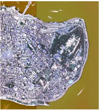
2.0 THE STUDY AREA

Suleymaniye, Istanbul, Turkey is the study area. It is a place of historical objects and monuments, which contains approximately 48,000 buildings, and an area of 1500 hectare. Planar rectangular faces constitute each building. The data are built in CAD and further converted to the geometry representation of Oracle Spatial 10g. The conversion is completed with a topology-geometry of the 2D and 3D spatial object.

Figure 1: The area of Suleymaniye

3.0 TERRESTRIAL LASER SCANNING

3.1 Data Acquisition

The 3D datasets were captured via Terrestrial Laser Scanning (TLS) system, Leica LS4500 (static and mobile). Initially, static system was used but then a more robust and quicker system was utilised, i.e. mobile laser scanning (MBL) system – due to project time constrained. The MBL consists of laser unit, IMU, and GPS and mounted on a vehicle. Huge amount of data were captured, it is the order of more than 50 Terra-byte and the data management system has been properly established by the laser-scanning unit at IMP (Istanbul Metropolitan Planning) and BIMTAS offices. For this project a new production organisation was established at BIMTAS using modern 3D mapping and computer technology. The terrestrial laser scanning group includes 24 staff, which uses the following technical equipment for data acquisition: five Leica scanners (four HDS4500 and one HDS3000), four ILRIS-3D scanners from Optech (Figure 2), four Topcon total stations for geodetic control point

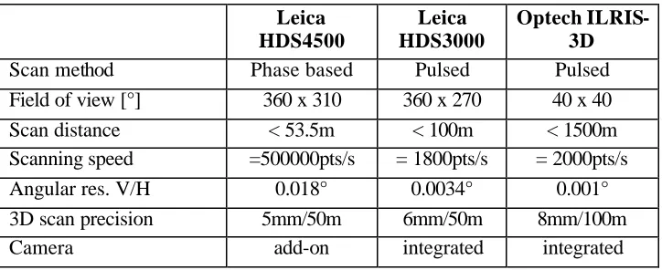
measurements and pre-calibrated SLR cameras Nikon D70 with 14mm and 28mm lenses for digital photogrammetric documentation. The technical specification of the terrestrial laser scanning systems used for this project are summarised in Table 1.

(3)

Table 1: Major specifications of the terrestrial laser scanning systems Leica HDS4500 Leica HDS3000 Optech ILRIS-3D

Scan method Phase based Pulsed Pulsed

Field of view [°] 360 x 310 360 x 270 40 x 40 Scan distance < 53.5m < 100m < 1500m Scanning speed =500000pts/s = 1800pts/s = 2000pts/s Angular res. V/H 0.018° 0.0034° 0.001° 3D scan precision 5mm/50m 6mm/50m 8mm/100m

Camera add-on integrated integrated

The three scanners use two different principles of distance measurement: Leica HDS4500 uses phase shift method, while Leica HDS3000 and ILRIS-3D scan with the time-of-flight method. In general it can be stated that phase shift method is fast but the signal to noise ratio depends on distance range and lighting conditions. If one compares scan distance and scanning speed shown in Table 1, it is obvious, that the scanner using the time-of-flight method can measure longer distances but is relatively slow compared to the phase shift scanner.

The HDS4500 measures distances up to 53m, while the HDS3000 and the ILRIS can measure up to 100m and 1500m, respectively. Due to the limited speed of 1500 or 4000 points per second and due to the limited field of view it quickly became clear that the ILRIS scanners and the HDS 3000 are not useful for the busy and narrow streets of the project area. These scanners are more suitable for the documentation of landmarks. Thus, all buildings were scanned with a scan resolution of ~15mm at the object using four HDS4500. For data processing of the scanned point clouds, which includes registration, geo-referencing and segmentation of the point clouds, five licenses of Cyclone 5.2 and four licenses of Polyworks 4.1 were used in the office.

Figure 3: Terrestrial laser scanners used: Leica HDS4500, Leica HDS3000, and Optech ILRIS-3D, target for registration and geo-referencing of scans.

For the scanning of the buildings, targets were used as control points for registration and geo-referencing of the scans from different scan stations as illustrated in Figure 3 (right). The targets have black-white quarters of a circle with a diameter of 126mm. To obtain centre positions of the targets, the targets were automatically fitted in the point cloud after manual pre-positioning using algorithms of the Leica Cyclone software.

3.2 Static terrestrial laser scanning

(4)

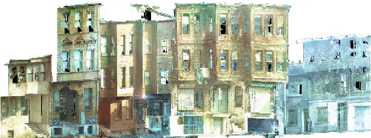
environment. As mentioned before the ILRIS-3D and HDS3000 scanner could not scan efficiently in the narrow streets due to the limitation in the field of view, distances that were too short and insufficient scanning speed. Furthermore, the registration of the point clouds of the ILRIS-3D caused problems with tilted scans from the same scan stations, and required matching with the Iterative Closest Point (ICP) algorithm and needed initial values for its computation. Consequently, the daily laser scanning was carried out with four, or sometimes with three, HDS4500. Figure 4 shows an example of a coloured point cloud of building facades at the Historic Peninsula.

Figure 4: Example of a coloured point cloud of building facades at the Historic Peninsula

In general, a satisfied spatial (geometrical) distribution of the targets on the object or around the object was guaranteed for the required description of the detailed object. The coordinates of all targets were determined by geodetic methods using total stations. The target-based registration and geo-referencing of the point clouds, which are acquired by the HDS4500 scanners, worked without any problems using five Cyclone software components as following: (a) registration of all scans and quality control of the result (check of residuals), and (b) geo-referencing using all control points including quality control by checking residuals.

80ha of the project area (of in total 1500ha) could be scanned within the first six months using the existing production capacity, which clearly indicated, that the scanning would need more than eight years for the entire area of the project, if this current scan rate of approximately 0.7ha per day could not be increased. It was obvious that the project deadline could not be met; therefore it was decided to increase the production rate by the integration of a mobile system.

3.3 Mobile terrestrial laser scanning

(5)

Figure 5: Sensor configuration on the mobile mapping van of VISIMIND AB

Due to problems with the reception of the GPS signal in the narrow streets of the Historic Peninsula control points were marked on the buildings every five meters along each side of the street (Figure 6). Some targets were removed or destroyed before scanning (Fig. 5 right) and were replaced by natural points such as window corners. Some targets were destroyed after scanning, but before the geodetic determination of the object coordinates, they also had to be replaced by natural points.

Figure 6: Distribution of control points in the streets for mobile terrestrial laser scanning (left), and destroyed target (right)

(6)

Figure 7: Geometric problems from direct geo-referencing of point clouds (from left to right: swinging façade, misfit at block corner, and deformation of a façade)

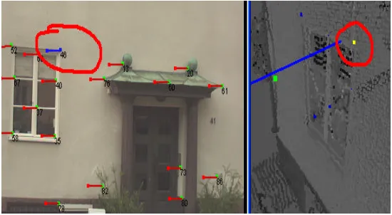
For problematic facades where control points were missing, VISIMIND recently developed with the so called ‘image tracking tool’ an automatic photogrammetric bundle adjustment enabling a bridging of longer distances without control points (Figure 8).

Figure 8: Image tracking tool for “problematic” facades without control points

The speed of data acquisition by terrestrial laser scanning with the mobile mapping system of VISIMIND could be increased significantly. 33 blocks could be scanned in 33 working days until the end of August 2007. Usually, scanning could be carried out five days per week. Consequently, the laser scanning of the remaining 50 blocks could be finished with the mobile system by November, 8th, 2007 with the improved total production rate of ~600m per hour, while post processing of the multiple sensor data took until January 2008. The production rate was mainly 1:10, i.e. for one hour scanning 10 hours post processing was needed. In total, 12 operators of the laser-scanning group were supporting the data post processing of the mobile mapping system during the major processing phase. Nevertheless, approximately 2% of the area (30ha) could not be scanned by mobile terrestrial laser scanning (TLS) due to traffic restrictions and environmental conditions. This remaining 2% of the total area must be scanned by static TLS at the end of the project in order to complete the data acquisition. At least two months will be needed for scanning by static TLS using all available laser-scanning systems.

3.4 Digital photogrammetry

(7)

acquisition, only the images of the integrated oblique and horizontal cameras (Figure 9) were used for mapping. The upper sideward looking camera is vertically rotated against the lower camera by approximately 34°, enlarging the vertical field of view of the camera system to approximately 86°, so that the camera system starts at an angle looking down to the street.

Figure 9: Oblique and horizontal camera integration in the mobile system (left), image taken by oblique camera (right)

3.5 Mapping of facades

The geo-referenced point clouds from the laser scanning group were used for line mapping of the facades in a plot scale 1:200. The point clouds were segmented by two people using Cyclone software before mapping (see Figure 10) to eliminate unnecessary points and to reduce the data volume to the requested minimal portions for the mapping software.

In this project generation of façade maps with 1:200 plot scale is required. This extreme demand corresponds to a standard deviation of the positions with 0.2mm in the map and 4cm in the object space, but this extreme accuracy is required only as relative accuracy; for the absolute accuracy a standard deviation of 0.5mm in the map, corresponding to 10cm in object space should be sufficient. As a tolerance limit of three times the standard deviation has been accepted. Therefore, the control point configuration and accuracy must always be checked to obtain this accuracy. While all problems of static and mobile scanning were solved, the delay in the control point determination was a bottleneck in the production.

Figure 10: Segmentation of point clouds.

(8)

laser scanning group: 80 ha with 32 operators in approximately 6 months. With regards the facade area, in total 81,000 m² could be finished in 39 days, which corresponds to 65 m² per person per day. The production rate could be increased from 60 m2 of facade/day/operator (March 2007) on average to 140 m2/day (October 2007), which is more than a factor of a 2 time increase. If one assumes in total 5 million m2 façade area for mapping of the Historic Peninsula, it corresponds to an estimated mapping time of approximately five years with 34 operators working on 210 days per year. This estimation indicated that the mapping could not be finished before the deadline of the project.

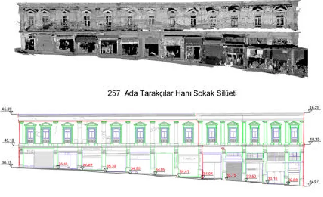
For data processing in Z-MAP all related data of the segmented part (point cloud, Nikon image(s), camera calibration file) was saved in one directory using the name of the block plus a suffix, e.g. 900_01. This block name is defined in the cadastre map. The HP workstations xw8200 used are equipped with dual XEON Processors (3.6 GHZ), 4 GB RAM and nvidea Graphic Cards with 256 MB RAM. For facade mapping the point cloud and one oriented image of the façade were used. Thus, the orientation of the photogrammetric image (usually recorded with the 14 mm lens) had to be determined by resection in space using at least five well distributed corresponding points (usually corners of windows) in the point cloud and in the image. For the adjustment of the spatial resection the calibration data of the pre-calibrated NIKON D70s are used. Usually the residuals of the control points were in the range of some millimetres, which indicated that sufficient results have been achieved. To carry out mapping with Z-MAP the images had to be rectified to the main plane of the facade. Therefore, the plane was defined by more than three points, which were measured in the point cloud and in the image. Thus, the photos were rectified to the main plane of the facades and shifted to parallel planes based on the point clouds. Based on the dense point clouds from the Leica HDS4500 scanners, the mapping was often possible without support of the photos, using just the grey values of the point cloud. Nevertheless, the colour photos are a significant support particularly for the detailed mapping of bricks and stones (see Figure 11). One major problem is the very detailed mapping of bricks and stones, which reduced the speed of mapping significantly. Unfortunately, the architects as the major clients could not be convinced to use digital orthophotos of the facades instead of the detailed maps in the scale of 1:200. An example of the final product from façade mapping is depicted in Figure 12, which is derived from 3D polylines as illustrated in Figure 13.

(9)

Figure 12: Part of the final product from façade mapping using terrestrial laser scanning data and photogrammetric images

Figure 13: Mapped 3D polylines of facades of a building block

4.0 3D SPATIAL DATABASE DEVELOPMENT

(10)

looking for applications that have one or more 3D GIS functionality. Due to the complexity of real-world spatial objects, various kinds of representations (e.g. vector, raster, constructive solid geometry, etc.), spatial data models (topology, and geometry) have been investigated and developed, including e.g. Pilouk, 1996; Zlatanova, 2000; and Kada et al, 2006. The management of 3D spatial objects has also been discussed in Orenstein (1986), Penninga (2005), Penninga et al. (2006), Penninga, and van Oosterom (2007), Pu (2005), Pu, and Zlatanova (2006), and Rigaux et al. (2002).

A universal and practical spatial data model that capable of addressing more than one application are rather hardly available – a model normally serves well for an application. One of the reasons is due to the complexity of the real world objects and situations. On the other hand, different disciplines emphasize different aspects of information e.g. including different in requirements and output. Thus, a data model could be considered good for a certain application but not so appropriate for other tasks. Different aspects and characteristics of real objects have led to the existence of several variations in object definition. The solution for these problems has directly referred to GIS standardization.

Current 3D GIS offer predominantly 2D functionality with 3D visualization and navigation capability. However, promising developments were observed in the DBMS domain where more spatial data types, functions and indexing mechanism were supported (PostGIS, 2008; Oracle Spatial, 2008). In this respect, DBMS are expected to become a critical component in developing of an operational 3D GIS. However, extended research and developments are needed to achieve native 3D support at DBMS level.

4.1. Existing Ge o-DBMS For 3D Modeling

Existing DBMS provides a SQL schema and functions that facilitate the storage, retrieval, update, and query of collections of spatial features. Most of the existing spatial databases support the object-oriented model for representing geometries. The benefits of this model is that it support for many geometry types, including arcs, circles, and different kinds of compound objects. Therefore, geometries could be modelled in a single row and single column. The model also able to create and maintain indexes, and later on, perform spatial queries efficiently. In the next section, Oracle Spatial will be discussed, in term of their characteristics, capabilities and limitations in handling multi-dimensional datasets.

4.2. Oracle Spatial

Oracle Spatial is designed to make spatial data management easier and more natural to users of location-enabled applications and geographic information system (GIS) applications. Once spatial data is stored in an Oracle database, it can be manipulated, retrieved, and related to all other data stored in the database. Types of spatial data (other than GIS data) that can be stored using Spatial include data from computer-aided design (CAD) and computer-aided manufacturing (CAM) systems. The Spatial also stores, retrieves, updates, or queries some collection of features that have both nonspatial and spatial attributes. Examples of nonspatial attributes are name, soil_type, landuse_classification, and part_number. The spatial attribute is a coordinate geometry, or vector-based representation of the shape of the feature.

(11)

4.3 Modeling 3D Solid Using MultiPolygon

In the Oracle Spatial object-relational model, a 3D solid object from 3D primitive is not possible. However, it could be done by implementing the MultiPolygon that bound a solid. The geometric description of a spatial object is stored in a single row and in a single column of object type SDO_GEOMETRY in a user-defined table. Any tables that have a column of type SDO_GEOMETRY must have another column, or set of columns, that defines a unique primary key for that table. Tables of this sort are sometimes referred to as geometry tables.

Oracle Spatial defines the object type SDO_GEOMETRY as:

CREATE TYPE sdo_geometry AS OBJECT ( SDO_GTYPE NUMBER,

SDO_SRID NUMBER,

SDO_POINT SDO_POINT_TYPE,

SDO_ELEM_INFO MDSYS.SDO_ELEM_INFO_ARRAY, SDO_ORDINATES MDSYS.SDO_ORDINATE_ARRAY);

An example implementing a 3D multipolygon (where the geometry can have multiple, disjoint polygons in 3D) is given in Appendix A.

The advantage of implementing the multipolygon in DBMS is that the integration between CAD and GIS is possible for 3D visualization, i.e. Oracle (or called Spatial) spatial schema is supported by Bentley MicroStation (2008) and Autodesk Map 3D (2009). This is due to the geometry column provided by Spatial is directly access to the 3D coordinates of the object, which allow the display tools retrieve spatial information from the geometry column.

4.4 The Implementation of Geo-DBMS

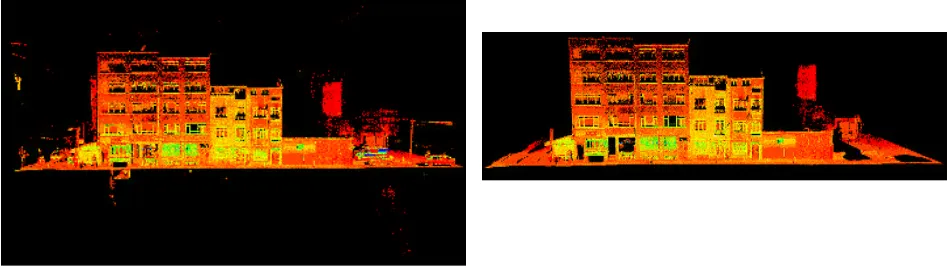
The implementation of geo-DBMS approach for laser scanner data is the main objective for this study. Thus, the 3D spatial objects were stored within Oracle Spatial environment. A 3D data type, i.e. MULTIPOLYGON was implemented for the spatial object. Figure 14 denotes one of the buildings captured using the laser scanning system (TLS).

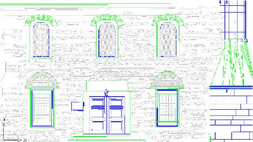
Although the complete coverage of the spatial data captured for the building could be obtained or acquired via the technique, the result of 3D point-clouds do not provide any semantic related to the building itself, in terms of spatial geometry, object’s behaviour (e.g. door is open from inside the building), or related attribute information (e.g. year of construction). Thus, the laser scanner data need to be processed in order to create useful spatial information. The first stage of the process is related to feature extraction and the discussion on this aspect could be found in Oude Elberink and Vosselman (2006); Teunissen (1991); Vosselman (2003). The result from object extraction and reconstruction is shown in Figure 15.

(12)

Figure 14: The raw datasets from laser scanner. (a) Exterior, and (b) Interior parts of 3D building

Figure 15: Feature extraction results from laser scanner data. (a) 3D view, and (b) 2D planar view

(a)

(b)

(13)

Table 2: A geometry table describes all related attribute columns

Table 3: The attribute information from spatial database

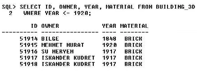
The geo-DBMS approach could provide spatial query related to the specific condition. For this research, the spatial could be performed using SQL language as shown in Table 4. In the following spatial query, the experiment defined all related historical building, which is constructed before the year of 1920.

Table 4: Sample spatial query

The methodology for the complete imple mentation is given in Figure 16. GEOMETRY

column from the database

(14)

Figure 16: The workflow

5.0 THE VISUALIZATION OF RETRIEVED 3D SPATIAL OBJECTS

Any spatial queries from database would only provide geometric and semantic information if the visualization factor is not considered. DBMS only provides a medium for the management of data set, and it certainly requires a front-end tool for visualizing for that information, as one perceives in the real world. The data from DBMS needs to be integrated into visualization tool so that it could be viewed as graphic. The 3D spatial data stores in the spatial column (within DBMS), and a connection needs to be built so that a display tool manages to access the spatial column and retrieve the data for 3D visualization.

It is also important to note that 3D objects need to be visualized in realism. With the benefit of the computer graphic technology, GIS could provide a good display with textures and colours. Some web application, e.g. Google Earth (GE) maintains the texture of spatial object over the Internet. Here, we used Autodesk Map 3D for displaying the 3D spatial object in this research.

5.1 Oracle Spatial and Map 3D schemas

In order to visualize Oracle spatial database successfully within the Map 3D environment, synchronization between Oracle spatial and Map 3D schema is required. However, sample spatial datasets within Oracle Spatial is illustrated in Table 5:

Raw data from laser scanner, 3D point-cloud

Feature extraction from laser scanner data

Implementation of Geo-DBMS approach Object reconstruction

& classification 1). Building blocks 2). Roads

3). Terrain

Implementation of Oracle Spatial as geo-DBMS platform

CREATE TABLE Solid3D ( ID number(11) not null,

shape mdsys.sdo_geometry not null);

(15)

Table 5: Extraction of geometry dataset

After datasets are inserted into Oracle database, the first stage of integration is to login into Map 3D (see Figure 17). The second stage of integration is to connect Oracle schema table into Map 3D’s schema administration. The Map 3D will prompt user for Oracle database login name and password. From the Oracle database lists, select the appropriate database for visualization.

Figure 17: Integration between Oracle Spatial and Map 3D

(16)

Figure 18: Import database, from Oracle Spatial to Map 3D

Figure 19: 3D display within Map 3D environment (without texture)

5.2 Real Texture Mapping

(17)

Figure 20: Real texture mapping, (a) before, and (b) after rectification

The initial 3D display of building block only manages to provide standard colours from Map 3D library. However, 3D textures could be attached into the spatial objects. This provides the realistic appearance of 3D building blocks as appeared in various city models. Figure 21 denotes the implementation of textures into the 3D spatial object (simple building without roof). Figure 22 denotes the similar implementation for complex building (with roof).

(18)

Figure 22: 3D display of complex building (with roof)

6.0 CONCLUDING REMARKS

The paper had discussed the implementation of geo-DBMS approach pertaining to the 3D spatial data modelling and management using the data generated from the laser scanning system. The discussions cover the implementation of 3D geometry from Oracle Spatial. However, there are several issues still need to be addressed in order to improve the current situation of 3D spatial modeling of objects from laser scanner data - objects reconstruction from the laser scanning system. At the moment, most systems only provide primitive means for object creation (i.e. manual technique). Our research experience shows that a lot of efforts still need to be done in order to create the 3D objects automatically. The other issue is related to the 3D primitives for the spatial database, e.g. polyhedron for building block, and tetrahedron for terrain modeling. This aspect can be solved by implementing the user-defined data type within the geo-DBMS environment. The most important issue for 3D spatial data modeling is the standardization and specification of GIS that related to the Open Geospatial Consortium (OGC standard), from feature extraction to final 3D display. The implementation of 3D spatial operations could also be done in geo-DBMS environment. The spatial operators should involve some procedures that able to use, query, create, modify, or delete spatial objects.

Other challenges and issues in the near future include the interoperability between different applications, data model, the integration between DBMS and visualization, and the real-time linkage between data model and data acquisition.

ACKNOWLEDGMENT

(19)

REFERENCES

Abdul-Rahman A, Zlatanova S, Coors V (2006). Lecture Note on geoinformation and cartography – Innovations in 3D Geo Information Systems, Springer-Verlag.

Abdul-Rahman A, Karas SR, Baz I, and Buyuksalih G (2008). Managing 3D Geospatial Objects – case study: Istanbul Historical Peninsula Region. Proceedings of International Conference on GIS for Developing Countries (GISDeco) 2008. 4 – 7th. June, Istanbul, Turkey.

Arens C, Stoter J, and van Oosterom PJM (2005). Modelling of 3D spatial objects in a geo-DBMS using a 3D primitive. Computers and Geosciences Journal, Vol. 31, No. 2, Elsevier, pp. 165-177

Autodesk Map 3D (2009). Available at http://usa.autodesk.com/. Bentley MicroStation (2008). Available at http://www.bentley.com/. Fritsch D (2003). Photogrammetric Week Workshop. Stuttgart, Germany Google Earth (2008). Available at http://earth.google.com/.

Kada M, Haala N, Becker S (2006). Improving the realism of existing 3D city model. In: Abdul-Rahman A, Zlatanova S, and Coors V (eds), Lecture Note on geoinformation and cartography – innovations in 3D Geo information systems, Springer-Verlag. pp. 405-415.

OGC (1999). Abstract specifications overview. Available at http://www.opengis.org.

OGC (1999a). OpenGIS simple features specification for SQL. Available at http://www.opengis.org. OGC (2001). The OpenGIS™ Abstract specification, topic 1: feature geometry (ISO 19107 Spatial Schema) Version 5.

Oracle Spatial (2008). Available at http://www.oracle.com/.

Orenstein J (1986). Spatial query processing in an object-oriented database system. In: Proceedings of 1986 ACM SIGMOD International Conference on Management of Data, pp. 326-336.

Oude Elberink S, and Vosselman G (2006). Adding the third dimension to a topographic database using airborne laser scanner data. Photogrammetric Computer Vision 2006. IAPRS, Bonn, Germany. Penninga F (2005). 3D topographic data modelling: why rigidity is preferable to pragmatism. In: Spatial Information Theory, Cosit’05, Vol. 3693 of Lecture Notes on Computer Science, Springer. pp 409-425.

Penninga F, van Oosterom PJM, Kazar BM (2006). A TEN-based DBMS approach for 3D topographic data modelling. In: Spatial Data Handling 2006.

Penninga F, and van Oosterom PJM (2007). A compact topological DBMS data structure for 3D topography. In: Fabrikant S, Wachowicz M (eds.), Lecture Notes in Geoinformation and Cartography. ISBN: 978-3-540-72384-4.

Pilouk M (1996). Integrated modelling for 3D GIS. PhD Thesis, ITC, The Netherlands. PostGIS (2008). Available at http://postgis.refractions.net/.

(20)

Pu S, and Zlatanova S (2006). Integration of GIS and CAD at DBMS level. In: E. Fendel E, Rumor M (eds), Proceedings of UDMS'06 Aalborg, Denmark, TU Delft, pp 9.61-9.71.

Rigaux P, Scholl M, Voisard A (2002). Spatial databases - with application to GIS. Morgan Kaufmann Publishers, San Francisco.

Teunissen PJG (1991). An integrity and quality control procedure for use in multi sensor integration. In: Proceedings of ION GPS-90, 19-21 September 1990, pp. 513-522, Colorado Springs, USA.

Vosselman G (2003). 3D reconstruction of roads and trees for city modelling. ISPRS working group III/3 workshop 3-D reconstruction from airborne laser scanner and InSAR data. IAPRS, Dresden, Germany, pp. 231-236.

(21)

APPENDIX A

The following SQL language denotes the implementation of 3D multipolygon for solid object.

CREATE TABLE Solid3D ( ID number(11) not null,

shape mdsys.sdo_geometry not null);

INSERT INTO Solid3D (ID, shape) VALUES (

1 SDO_GEOMETRY(3007, -- 3007 indicates a 3D multipolygon

NULL, -- SRID is null

NULL, -- SDO_POINT is null

SDO_ELEM_INFO_ARRAY( -- the offset of the polygon

1, 1003, 1, 16, 1003, 1, 31, 1003, 1, 46, 1003, 1, 61, 1003, 1, 76, 1003, 1), SDO_ORDINATE_ARRAY(

4,4,0, 4,0,0, 0,0,0, 0,4,0, 4,4,0, -- 1st_{lower polygon}