Inaugural - Dissertation

(1)

Inaugural - Dissertation

zur

Erlangung der Doktorwürde

der

Naturwissenschaftlich-Mathematischen Gesamtfakultät

der

Ruprecht - Karls - Universität

Heidelberg

vorgelegt von

Diplom-Mathematiker

Markus Fischer

aus Berlin

(2)

(3)

Discretisation of continuous-time stochastic

optimal control problems with delay

Gutachter:

Prof. Dr. Markus Reiß

Universität Heidelberg

Prof. Salah-Eldin A. Mohammed

(4)

(5)

i

Abstract

In the present work, we study discretisation schemes for continuous-time stochastic optimal control problems with time delay. The dynamics of the control problems to be approximated are described by controlled stochastic delay (or functional) differential equations. The value functions associated with such control problems are defined on an infinite-dimensional function space.

The discretisation schemes studied are obtained by replacing the original control pro-blem by a sequence of approximating discrete-time Markovian control propro-blems with finite or finite-dimensional state space. Such a scheme is convergent if the value functions as-sociated with the approximating control problems converge to the value function of the original problem.

Following a general method for the discretisation of continuous-time control problems, sufficient conditions for the convergence of discretisation schemes for a class of stochastic optimal control problems with delay are derived. The general method itself is cast in a formal framework.

A semi-discretisation scheme for a second class of stochastic optimal control problems with delay is proposed. Under standard assumptions, convergence of the scheme as well as uniform upper bounds on the discretisation error are obtained. The question of how to numerically solve the resulting discrete-time finite-dimensional control problems is also addressed.

(6)

Zusammenfassung

In der vorliegenden Arbeit untersuchen wir Schemata zur Diskretisierung von zeitsteti-gen stochastischen Kontrollproblemen mit Zeitverzögerung. Die Dynamik solcher Probleme wird von gesteuerten stochastischen Differentialgleichungen mit Gedächtnis beschrieben. Die zugehörigen Wertfunktionen sind auf einem unendlich-dimensionenalen Funktionen-raum definiert.

Man erhält die Diskretisierungsschemata, die wir betrachten, indem man das Ausgangs-problem durch eine Folge approximierender zeitdiskreter Markovscher KontrollAusgangs-probleme ersetzt, deren Zustandsraum endlich-dimensional oder endlich ist. Ein solches Schema ist konvergent, wenn die Wertfunktionen der approximierenden Steurungsprobleme gegen die Wertfunktion des ursprünglichen Problems streben.

Indem wir eine allgemeine Methode zur Diskretisierung zeitstetiger Kontrollprobleme anwenden, erhalten wir hinreichende Bedingungen für die Konvergenz von Diskretisierungs-schemata für eine Klasse von stochastischen Steuerungsproblemen mit Zeitverzögerung. Die Methode zur Konvergenzanalyse selbst wird in einen formalen Rahmen gefasst.

Wir führen dann ein Semidiskretisierungsschema für eine zweite Klasse von stochasti-schen Steuerungsproblemen mit Zeitverzögerung ein. Unter üblichen Annahmen werden die Konvergenz des Schemas, aber auch gleichmäßige obere Schranken für den Diskreti-sierungsfehler hergeleitet. Schließlich widmen wir uns der Frage, wie die resultierenden endlich-dimensionalen Steuerungsprobleme numerisch gelöst werden können.

(7)

iii

Danksagung

Für den Vorschlag des Gebietes, in das die vorliegende Arbeit fällt, und die Betreuung und ununterbrochene Unterstützung in allen fachlichen und auch außerfachlichen Fragen danke ich Prof. Markus Reiß. Mein Dank gebührt Prof.ssa Giovanna Nappo von der Universi-tät “La Sapienza” für die fruchtbare Zusammenarbeit und ihre Gastfeundschaft während meines Aufenthalts in Rom von April bis September 2006. Für die Unterstützung bei der Organisation dieses Aufenthalts danke ich Prof. Peter Imkeller.

Den Mitgliedern der Forschungsgruppe “Stochastische Algorithmen und Nichtparame-trische Statistik” am Weierstraß Institut (WIAS) in Berlin und den Mitgliedern der Sta-tistikgruppe an der Universität Heidelberg danke ich für die angenehme gemeinsam ver-brachte Zeit.

Für wertvolle Hinweise zur Theorie deterministischer Kontrollprobleme danke ich Prof. Maurizio Falcone. Für fachliche Gespräche, Anregungen und Unterstützung danke ich Stefan Ankirchner, Christian Bender, Christine Grün, Jan Johannes, Alexander Linke, Jan Neddermeyer, Eva Saskia Rohrbach und Karsten Tabelow.

Finanzielle Unterstützung von Seiten der Deutschen Forschungsgemeinschaft (DFG) und des ESF-Programms “Advanced Methods in Mathematical Finance” erkenne ich dan-kend an.

(8)

(9)

Introduction

In this thesis, discretisation schemes for the approximation of continuous-time stochastic optimal control problems with time delay in the state dynamics are studied. Optimal control problems of this kind are infinite-dimensional control problems in a sense to be made precise below; they arise in engineering, economics and finance, among others.

We will derive results about the convergence of discretisation schemes. For a more specific semi-discretisation scheme, a priori bounds on the discretisation error will also be obtained. Such results are useful in the numerical solution of the original control problems. Section 1.1 presents the class of optimal control problems we will be concerned with. In Section 1.2, some examples of optimal control problems with delay are given. Section 1.3 provides an overview over approaches and some results from the literature related to the discretisation of continuous-time optimal control problems – with or without delay. The organisation of the main part of the present work, its aim and scope are specified in Section 1.4

1.1 Stochastic optimal control problems with delay

Here, we introduce the type of optimal control problems we will be concerned with in this thesis. An optimal control problem is composed of two parts: a controlled system and a performance criterion. Given an initial condition of the system and a strategy, the system produces a unique output. A numerical value is assigned to each output according to the performance criterion. In this way, the “performance” of any strategy for any given initial condition is measured. The objective is to find strategies which perform as good as possible, and to calculate optimal performance values.

A controlled system is usually modelled as a discrete- or continuous-time (parametrised) dynamical system. In continuous time, controlled systems are often described by some kind of differential equation. The continuous-time controlled systems we are interested in, here, are modelled as stochastic (or deterministic) delay differential equations. We describe this class of equations in Subsection 1.1.1; a standard reference is Mohammed (1984). In Subsection 1.1.2, the class of stochastic optimal control problems with delay we study in this work is introduced. If the time delay is zero, then those problems reduce to ordinary stochastic optimal control problems. For this latter class of problems a well-developed theory exists; see, for instance, Yong and Zhou (1999) or Fleming and Soner

(14)

(2006). Basic optimality criteria, in particular the Principle of Dynamic Programming, are also mentioned in Subsection 1.1.2.

1.1.1 Stochastic delay differential equations

An ordinary Itô stochastic differential equation (SDE) is an equation of the form

(1.1) dX(t) = b t, X(t)dt + σ(t, X(t)dW(t), t≥0,

wherebis thedrift coefficient,σthediffusion coefficientandW(.)a Wiener process. When the diffusion coefficient σ is zero, then Equation (1.1) takes on the form of an ordinary differential equation (ODE).

Let the state space be Rd. The unknown function X(.) in Equation (1.1) is then an Rd-valued stochastic process with continuous or càdlàg1 trajectories. The drift coefficient

b is a function [0,∞) ×_Rd _→

Rd, the diffusion coefficient σ a matrix-valued function

[0,∞)×Rd → Rd×d1, and W is a d1-dimensional Wiener process defined on a filtered

probability space (Ω,F,P) adapted to the filtration (Ft)t≥0. In the notation, we often

omit the dependence on ω∈Ω.

Equation (1.1) is to be understood as an integral equation. Standard assumptions on the coefficients b,σ guarantee that the initial value problem

(1.2) X(t) = ( X(0) + Rt 0 b s, X(s) ds + Rt 0σ(s, X(s) dW(s), t >0, x, t= 0,

possesses, for each x∈Rd, a uniquestrong solution, that is, there is a unique (up to

indis-tinguishability) _Rd-valued stochastic process X = (X(t))t≥0 with continuous (or càdlàg)

trajectories which is defined on (Ω,F,P) and adapted to the filtration (F_t)t≥0 such that

Equation (1.2) is satisfied. The initial condition may also be stochastic, namely an F0

-measurable_Rd-valued random variable.

Standard assumptions guaranteeing (strong) existence and uniqueness of solutions to Equation (1.2) are that b, σ are jointly measurable, Lipschitz continuous in the second variable (uniformly in the first) and that they satisfy a condition of sublinear growth in the second variable uniformly in the first; see paragraph 5.2.9 in Karatzas and Shreve (1991: p. 289), for example.

An important property of solutions of SDEs is that they areMarkov processes w. r. t. the given filtration. Another equally important property is that they are continuous semi-martingales with semi-martingale decomposition given by the SDE itself.

In addition to the notion of strong solution, there is the notion of weak solution to an SDE. While strong solutions must live on the given probability space and must be adapted to the given filtration, weak solutions are only required to exist on some suitable stochastic basis; for example, the given filtration may be the one induced by the driving Wiener process, but solutions exist only when they are adapted to some larger filtration. Thus, there are two notions of existence and also two notions of uniqueness for an SDE, cf. Karatzas and Shreve (1991: Sects. 5.2 & 5.3).

1

(15)

1.1. STOCHASTIC OPTIMAL CONTROL PROBLEMS WITH DELAY 3

The basic existence and uniqueness results carry over to the case of random coefficients, that is,b,σ are defined on[0,∞)×Rd×Ω, providedb,σ are(Ft)-adapted.2 A controlled

SDE can be represented in the form

(1.3) dX(t) = b t, X(t), u(t)dt + σ(t, X(t), u(t)dW(t), t≥0,

where u(.) is a control process, that is, an (F_t)-adapted function [0,∞)×Ω → Γ. Here, Γ is a separable metric space, called the space of control actions. The coefficients in Equation (1.3) are deterministic functions [0,∞)×_Rd_×_Γ_→

Rd and [0,∞)×Rd×Γ→ Rd×d1, respectively. For any given control processu(.), however,b(., ., u(.)),σ(., ., u(.))are

adapted random coefficients.

A control processu(.)such that the initial value problem corresponding to the controlled equation, here Equation (1.3), has a unique solution for each initial condition of interest will be called anadmissible strategy or, simply, astrategy.

Throughout this thesis, we will represent control processes and strategies as (Γ-valued) functions defined on[0,∞)×Ω, that is, defined on the product of time and scenario space. In the deterministic case, control processes reduce to functions [0,∞) → Γ, so-called

open-loop controls. In the literature, control processes are often represented as feedback controls, that is, as deterministic functions defined on the product of time and state space. This representation, though being “natural” for the control of Markov processes, leads to technical difficulties already for discrete-time control problems, see Bertsekas and Shreve (1996). Feedback controls give rise to control processes in the form considered here.

Systems with delay are characterised by the property that their future evolution, as seen from any instant t, depends not only on t and the current state at t (and possibly the control), but also on states of the system a certain amount of time into the past. We will assume throughout that the system has bounded memory; thus, there is some finite r >0 such that the future evolution of the system as seen from time t depends only on t and system states over the period [t−r, t]. The parameterr is the maximal length of the memory or delay.

Stochastic delay differential equations (SDDEs) model systems with delay. The drift and diffusion coefficient of an SDDE are functions of time and trajectory segments (and, possibly, the control action). For an_Rd-valued functionψ=ψ(.)living on the time interval [−r,∞), thesegment of lengthr at timet∈[0,∞) is the function

ψt: [−r,0]→Rd, ψt(s) := ψ(t+s), s∈[−r,0].

Ifψis a continuous function, then the segmentψtat timetis a continuous function defined

on [−r,0]. Likewise, if ψ is a càdlàg function, then the segment ψt at time t is a càdlàg

function defined on[−r,0].

Accordingly, if(X(t))t≥−r is anRd-valued stochastic process with continuous

trajecto-ries, then the associated segment process(Xt)t≥0is a stochastic process taking its values in C:=C([−r,0],Rd), the space of allRd-valued continuous functions on the interval[−r,0].

In this work, the space C will always be equipped with the supremum norm induced by the standard norm onRd.

2

Strictly speaking, the statement about SDEs with random coefficients is true only if existence and uniqueness are understood in the strong sense. The notions of weak existence and weak uniqueness make sense also for solutions to controlled SDEs (with or without delay), cf. Section 3.1.

(16)

The segment process associated with an_Rd-valued stochastic process with càdlàg tra-jectories takes its values in the space D0:=D([−r,0],Rd)of allRd-valued càdlàg functions

on [−r,0]. We will refer to the space of trajectory segments as the segment space. As segment space we will choose either D0 or C. Notice that both spaces depend on the

di-mensiondand the maximal length of the delayr; bothdandr may vary. In the notation just introduced, an SDDE is of the form

(1.4) dX(t) = b t, Xt

dt + σ(t, Xt

dW(t), t≥0.

The coefficients b, σ are now functions defined on [0,∞)× D or, in the case of random coefficients, on [0,∞)× D ×Ω, where D is the segment space. In order to obtain unique solutions, as initial condition we have to prescribe not a pointx∈Rd, but an initial segment

ϕ ∈ D. The initial segment might also be stochastic, namely a D-valued F₀-measurable random variable.

Let the segment space be the space C of continuous functions. Theorem II.2.1 in Mohammed (1984: p. 36) gives sufficient conditions such that, for each initial segment ϕ∈ C, the initial value problem

(1.5) X(t) = ( X(0) + R₀tb s, Xs ds + R₀tσ(s, Xs dW(s), t >0, ϕ(t), t∈[−r,0],

possesses a unique strong solution. Sufficient conditions are that the coefficients b,σ are measurable, are Lipschitz continuous in their segment variable under the supremum norm onC uniformly in the time variable, satisfy a linear growth condition and, in case they are random, are (F_t)-progressively measurable.

Existence and uniqueness results for SDDEs can also be derived from the existence and uniqueness results for general functional SDEs as given, for instance, in Protter (2003: Ch. 5). There, the coefficients of the SDE are allowed to be random and to de-pend on the entire trajectory of the solution from time zero up to the current time. Initial conditions, however, are not trajectory segments, but points in _Rd (or _Rd-valued random variables). Hence, to transfer the results, the drift and diffusion coefficient of the SDDE have to be redefined according to the given initial condition.

Acontrolled SDDE can be represented in the form (1.6) dX(t) = b t, Xt, u(t)

dt + σ(t, Xt, u(t)

dW(t), t≥0,

whereu(.)is aΓ-valued control process as above andb,σare deterministic functions defined on[0,∞)× D ×Γ. Existence and uniqueness are again a consequence of the general results applied to the random coefficients b(., ., u(.)),σ(., ., u(.)).

Observe that, in Equation (1.6), there is no delay in the control. At time t >0, the coefficients b, σ depend on u(t), and u(t) is F_t-measurable. Systems with delay in the control are outside the scope of the present work. Some kind of implementation delay, however, can be captured. Let w be some measurable functionΓ→ _Rl_{. We can now add}

l additional dimensions to the state space_Rd and consider an SDDE of the form dX(t) = ˜b t, Xt, Yt, u(t) dt + ˜σ(t, Xt, Yt, u(t) dW(t), dY(t) = w u(t) dt,

(17)

whereX(.) represents the first d components and Y(.) the remaining l components. The coefficients ˜b, σ˜ do not directly depend on the trajectory of u(.), but, through Yt, on

segments of the process (R₀tw(u(s))ds)t≥0 (and the initial segment Y0); ˜b, σ˜ may, for

example, be functions of the difference Y(t−δ)−Y(t−r), where δ ∈ [0, r). In this way,

distributed implementation delay can be modelled.

The solution of an SDDE like Equation (1.4) is, in general, not a Markov process. Suppose the coefficients of the SDDE are deterministic and uncontrolled (or else a con-stant control is applied), and let X(.) be a solution process. Then the segment pro-cess (Xt)t≥0 associated with X(.)enjoys the Markov property, cf. Theorem III.1.1 in

Mo-hammed (1984: p. 51). The Markov semigroup of linear operators induced by the transition probabilities of the segment process is weakly, but not strongly continuous. In particular, only the weak infinitesimal generator exists. A representation of the weak infinitesimal generator on a subset of its domain as a differential operator can be derived, cf. Theo-rem III.4.3 in Mohammed (1984: pp. 109-110).

The solution of an SDDE like Equation (1.4), although generally not a Markov process, is an Itô diffusion and a continuous semi-martingale (after time zero), and the Itô formula is applicable as usual. However, the usual Itô formula does not apply to the segment process. It is possible to develop an Itô-like calculus also for the segment processes associated with solutions of SDDEs, see Hu et al. (2004) and Yan and Mohammed (2005).

In this thesis, the driving noise process of the continuous-time systems will always be a Wiener process. Extensions of some of the results of this thesis, in particular the convergence analysis of Section 2.3, to systems driven by more general Lévy processes are possible.

In Chapters 2 and 3, we will be concerned with the discretisation of controlled systems with delay; here, we give some references to works concerned with the discretisation of un-controlled systems with delay. An overview of numerical methods for unun-controlled SDDEs is given in Buckwar (2000). The simplest discretisation procedure is the Euler-Maruyama scheme. The work by Mao (2003) gives the rate of convergence for this scheme provided the SDDE has globally Lipschitz continuous coefficients and the dependence on the segments is in the form of generalised distributed delays; Proposition 3.3 in Section 3.2 of the present work provides a partial generalisation of Mao’s results and uses arguments similar to those in Calzolari et al. (2007). The most common first order scheme is due to Milstein; see Hu et al. (2004) for the rate of convergence of this scheme applied to SDDEs with point delay.

1.1.2 Optimal control problems with delay

Recall that an optimal control problem is composed of a controlled system and a per-formance criterion. In what follows, the controlled system will always be described by a controlled SDDE like Equation (1.6) in Subsection 1.1.1. As initial condition, an ele-ment of the segele-ment space D has to be prescribed; the segment space D will be either

C := C([−r,0],Rd) or D0 := D([−r,0],Rd). When, in addition to the initial segment

(18)

initial condition (t0, ϕ) under control processu(.)is determined by (1.7) X(t) = ( ϕ(0) + R₀tb t0+s, Xs, u(s) ds + R₀tσ(t0+s, Xs, u(s) dW(s), t >0, ϕ(t), t∈[−r,0],

provided a unique solution X = Xt0,ϕ,u _{exists. Notice that the solution process} _X₍_.₎ _is

defined over time [−r,∞), and the evolution of the system starts at time zero. The initial timet0 only appears in the time argument of the coefficients.

The performance criterion is usually given in terms of a cost functional. The cost functionals we will consider are of the form

(1.8) (t0, ϕ), u(.) 7→ E Z τ 0 f t0+s, Xs, u(s) ds + g Xτ , where X = Xt0,ϕ,u _{is the solution to Equation (1.7) with initial condition} ₍_t

0, ϕ) under

strategy u(.) and τ is the remaining time, which may depend on t0 and Xt0,ϕ,u. The

functionsf,g are called thecost rateand terminal cost, respectively; they may depend on segments of the solution process; in general, f is a function[0,∞)× D ×Γ→ _R, while g is a function D →_R.

Two versions of (1.8) will play a role. The first version gives rise to optimal control problems with finite time horizon. Choose T >0, the deterministic time horizon, and set τ:=T−t0. For the second version, choose a bounded open setO ⊂Rd, letˆτObe the time

of first exit of Xt0,ϕ,u _from_O _{and set} _τ_{:= ˆ}_τ

O∧(T−t0), where T ∈(0,∞]. This leads to

optimal control problems withrandom time horizon.

Let T > 0 be finite, and let τ in (1.8) be T−t0. Denote by U the set of admissible

strategies, that is, the set of all those control processes u(.) such that the initial value problem (1.7) yields a unique solution and the expectation in (1.8) a finite value for each initial condition (t0, ϕ) ∈ [0, T]× D. Let the function J: [0, T]× D × U →R be defined

according to (1.8). Then J is the cost functional of an optimal control problem with finite time horizon.

Given an optimal control problem, there is a twofold objective: determine the minimal costs and find an optimal strategy for any initial condition. A strategyu∗ is optimal for a given initial condition (t0, ϕ)iff

(1.9) J(t0, ϕ, u∗) = inf

u∈UJ(t0, ϕ, u).

Existence of optimal strategies is not always guaranteed. Let us assume that the right hand side of Equation (1.9) is finite for all initial conditions (which is not necessarily the case). A direct minimisation of J(t0, ϕ, .) over the setU is usually not possible. Observe

that initial conditions are time-state pairs; here, “states” are segments, that is, continuous or càdlàg functions on [−r,0].

A simple, yet fundamental approach, associated with the work of R. Bellman, to solving the dynamic optimisation problem is as follows. Introduce the function which assigns the minimal costs to each time-state pair. This function is called the value function. The values of the value function are, of course, unknown at this stage. If the system, the set of strategies and the cost functional have a certain additive structure in time, then the value function obeys Bellman’s Principle of Optimality or, as it is also called, the Principle of

(19)

Dynamic Programming (PDP). Let V denote the value function of some optimal control problem; thus, V is a function I × S → R, where I is a time interval and S the “state

space”. Bellman’s Principle then states thatV satisfies (1.10) V(t, x) = T_t,r V(r, .)

(t, x) for allx∈ S, t, r∈I, t≤r,

where(Tt,r)is a two-parameter semigroup of monotone operators, calledBellman operators;

see Fleming and Soner (2006: Sect. II.3) for this abstract formulation of the PDP. In the case at hand, the value function is defined by

V : [0, T]× D →R, V(t0, ϕ) := inf

u∈UJ(t0, ϕ, u).

(1.11)

The Principle of Dynamic Programming takes on the form

(1.12) V(t0, ϕ) = inf u∈UE Z t 0 f t0+s, Xsu, u(s) ds + V(t0+t, Xtu) , 0≤t≤T−t0,

whereXu is the solution to Equation (1.7) under control process u with initial condition (t0, ϕ). The minimisation on the right hand side of Equation (1.12) could be restricted to

strategies defined on the time interval[0, t].

Observe that the validity of the PDP has to be verified for each class of optimal control problems. For finite horizon stochastic (and deterministic) optimal control problems with delay, the PDP is indeed valid, see Larssen (2002) and also Appendix A.1 for the precise statement. The Markov property of the segment processes associated with solutions to Equation (1.7) under certain strategies is essential for the validity of the PDP in the form of Equation (1.12).

Notice that an optimal control problem with delay is, generally, infinite-dimensional in the sense that the corresponding value function lives on an infinite-dimensional function space, namely the segment space.

When the controlled processes are controlled Markov processes with finite-dimensional state space and the value function is sufficiently smooth, then the PDP in conjunction with Dynkin’s formula allows to derive a partial differential equation (PDE) which is solved by the value function. Such a PDE, which involves the family of infinitesimal generators associated with the controlled Markov processes and characterises the value function, is called Hamilton-Jacobi-Bellman equation (HJB equation). In general, the value function need not be sufficiently smooth; consequently, the HJB equation does not necessarily possess classical solutions. Viscosity solutions provide the “right” generalisation of the concept of solution for HJB equations, see Fleming and Soner (2006).

In principle, it is possible to derive an HJB equation and define viscosity solutions also for controlled Markov processes with infinite-dimensional state space. See Chang et al. (2006) for results in this direction in connection with controlled SDDEs; also cf. Subsection 1.2.1. While, in Chapter 3, we will make extensive use of the PDP, we will not need any kind of HJB equation.

Let us also mention the fact that knowledge of the value function of an optimal control problem enables us to construct optimal or “nearly” optimal strategies. When time is discrete and the space of control actionsΓis finite or compact, then optimal strategies can be constructed in feedback form (and for each initial condition). We will return to this point in Section 3.4.

(20)

A second fundamental approach to optimal control problems is via Pontryagin’s Max-imum Principle, see Yong and Zhou (1999: Chs. 3 & 7) for the case of finite-dimensional controlled SDEs. Pontryagin’s Principle provides necessary conditions which an optimal strategy and the associated optimal process (if such exist) have to satisfy in terms of the so-called adjoint equations, which evolve “backwards” in time. Under certain additional assumptions, the necessary conditions become sufficient. Versions of this principle for the control of deterministic systems with delay exist, cf. the example in Subsection 1.2.2. For stochastic control problems with delay of a special form, a version of the Pontryagin Max-imum Principle is derived in Øksendal and Sulem (2001). For the results of this thesis, we will not rely on the Maximum Principle.

We have not made precise any assumptions on the coefficients of the control problems introduced above. This will be done in Subsection 2.3.1 and Section 3.1, respectively, where we specify the classes of continuous-time control problems to be approximated.

1.2 Examples of optimal control problems with delay

Some examples of continuous-time optimal control problems with delay, mostly from the lit-erature, are given in this section. Control problems with linear dynamics and a “quadratic” cost criterion are well-studied in many settings. In Subsection 1.2.1, we cite results con-cerning the representation of optimal strategies for a class of linear quadratic regulators with point as well as distributed delay. In Subsection 1.2.2, a simple deterministic prob-lem with point delay modelling the optimal allocation of production resources is presented. Subsection 1.2.3 describes a stochastic optimal control problem with delay which may arise in finance when pricing derivatives that depend on market external processes. Special cases of optimal control problems with delay are really equivalent to finite-dimensional control problems without delay. Subsection 1.2.4 contains results from the literature about those reducible problems.

A further example is the deterministic infinite horizon model of optimal economic growth studied in Boucekkine et al. (2005). Optimal control problems also arise in finance when the asset prices in a financial market are modelled as SDDEs, see Øksendal and Sulem (2001), for instance.

1.2.1 Linear quadratic control problems

When the system dynamics are linear in the state as well as in the control variable, the noise is additive and the cost functional has a quadratic form over a finite or infinite time horizon, then it is possible to derive a representation of the optimal strategies of the control problem. Such control problems are referred to as linear quadratic problems or linear quadratic regulators. Optimal strategies are given in feedback form; the representation involves the solution of an associated system of deterministic differential equations, the so-called Riccati equations. This is the case not only for finite-dimensional stochastic and deterministic systems, but also for systems described by abstract evolution equations (cf. Bensoussan et al., 2007).

Here, we just cite a result for finite horizon linear quadratic systems with one point and one distributed delay and additive noise, see Kolmanovskiˇı and Shaˇıkhet (1996: Ch. 5).

(21)

1.2. EXAMPLES OF OPTIMAL CONTROL PROBLEMS WITH DELAY 9

We consider the time-homogeneous case. The dynamics of the control problem are given by the affine-linear equation

dX(t) =A X(t)dt + A1X(t−r)dt + Z 0 −r G(s)X(t+s)ds dt + B u(t)dt + σdW(t), t >0, (1.13)

wherer >0is the delay length, W(.) a d1-dimensional standard Wiener process adapted

to the filtration(F_t)t≥0,u(.)a strategy, σ is a d×d1-matrix,A,A1 ared×d-matrices,G

is a bounded continuous function[−r,0]→_Rd×d_{, and}_B _{is a} _d_×_l_-matrix.

The strategy u(.) in Equation (1.13) is any _Rl-valued (F_t)-adapted square integrable process. Let U denote the set of all such processes. Let D0:= D([−r,0],Rd) denote the

space of all _Rd-valued càdlàg functions on[−r,0]. Givenϕ∈D0 and a strategyu(.) ∈ U,

there is a unique (up to indistinguishability)d-dimensional càdlàg processX(.) =Xϕ,u(.) such that Equation (1.13) is satisfied and X(t) =ϕ(t) for allt∈[−r,0].

Let T >0 be the deterministic time horizon. The quadratic cost functional (for fixed initial time zero) is the function J:D0× U →Rgiven by

(1.14) J(ϕ, u) := E XT(T)C X(T) + Z T 0 XT(t) ˜C X(t) +uT(t)M u(t)dt , whereC,C˜are positive semi-definited×d-matrices andM is a positive definitel×l-matrix. The associated value function (at initial time zero) is defined by

V(ϕ) := inf

u∈UJ(ϕ, u), ϕ∈D0.

For the control problem determined by (1.13) and (1.14), a version of the Hamilton-Jacobi-Bellman equation3allows to derive a representation in feedback form of the optimal strategies. Define the functionu0: [0, T]×D0 →Rl by

u0(t, ϕ) := −M−1BT P(t)ϕ(0) + Z 0 −r Q(t, s)ϕ(s)ds , whereP,Qare matrix-valued functions[0, T]→_Rd×d_and_[0_{, T}_]_×_[₋_r,_0]_→

Rd×d,

respec-tively. The functionsP,Qare determined by the following system of differential equations, which involves, in addition, the unknown functionsR: [0, T]×[−r,0]×[−r,0]→_Rd×d_and

g: [0, T]→_R: d dtP(t) +A T_P₍_t_{) +}_P₍_t₎_A₍_t_{) +}_Q₍_t,_{0) +}_QT₍_t,_{0) + ˜}_C ₌_P₍_t₎_{B M}−1_BT_P₍_t₎_, (1.15) ∂ ∂t− ∂ ∂s Q(t, s) +P(t)G(t, s) +ATQ(t, s) +R(t,0, τ) =P(t)B M−1BTQ(t, s), ∂ ∂t− ∂ ∂s− ∂ ∂τ R(t, s, τ) +GT(t, s)Q(t, τ) +QT(t, s)G(t, τ) =QT(t, s)B M−1BTQ(t, τ), d dtg(t) + trace σ T_P₍_t₎_σ = 0, t∈[0, T], s, τ ∈[−r,0], 3

The derivation of the HJB equation in Kolmanovskiˇı and Shaˇıkhet (1996: Ch. 5) is not completely rigorous; see Chang et al. (2006) and the references therein for a more careful treatment. The development there starts from the expression for the weak infinitesimal generator of the segment process as derived in Mohammed (1984).

(22)

with boundary conditions

P(T) = C, R(T, s, τ) = 0, Q(T, s) = 0, (1.16)

g(T) = 0, P(t)A1 = Q(t,−r), AT1Q(t, s) = R(t,−r, s),

t∈[0, T], s, τ ∈[−r,0].

Equations (1.15) can be shown to possess a unique continuously differentiable solution (P, Q, R, g) under boundary conditions (1.16), see Theorem 5.2.1 in Kolmanovskiˇı and Shaˇıkhet (1996: p. 124). It is also shown that u0 is indeed an optimal feedback control.

This means the following. Letϕ∈D0, and letX∗=X∗,ϕ be the unique solution to

(1.17) X∗(t) =          ϕ(0) + R₀t A X∗(τ) + A1X∗(τ−r) + R0 −rG(s)X ∗₍_τ₊_s₎_ds_dτ + Rt 0 B u0 τ, X ∗ τ) dτ + σ W(t) ift >0, ϕ(t) ift∈[−r,0].

Recall the notationX_τ∗for the segment ofX∗(.)at timeτ. Observe thatu0is Lipschitz

con-tinuous (in supremum norm) in its segment variable, whence strong existence and unique-ness of the solution X∗ are guaranteed. Indeed, due to the form of u0, Equation (1.17) is

an affine-linear uncontrolled SDDE, and X∗ can be expressed by a variation-of-constants formula. Set u∗(t) :=u0(t, X∗), t≥0. Then it holds that J(ϕ, u∗) = V(ϕ), that is, u∗ is

an optimal strategy and X∗ is the optimal process for the given initial condition ϕ. In special cases, Equations (1.15) can be solved explicitly. For general linear quadratic problems, they may serve as a starting point for the numerical computation of optimal strategies and minimal costs.

1.2.2 A simple model of resource allocation

The following finite-horizon deterministic problem can be interpreted as a simplified model of optimal resource allocation; see Bertsekas (2005: Ex. 3.1.2, 3.3.2) for the non-delay case. Let T >0 be the time horizon, letr ∈[0, T) be the length of the time delay, and c >0 a parameter. The dynamics of the model are given by

(1.18)

(

˙

x(t) = c u(t)x(t−r), ift >0, x(t) = ϕ(t), ift∈[−r,0],

where the initial pathϕis inC+:=C([−r,0],(0,∞)); ifr = 0, thenϕis just a positive real

number. An admissible strategy u(.) is any element of the set U of all Borel measurable functions[0,∞)→[0,1].

The initial time will be fixed and equal to zero. The objective is to maximise, for each initial segmentϕ∈ C+, the cost functional

˜

J(ϕ, u) :=

Z T 0

1−u(t)x(t−r)dt over u∈ U. Clearly, this is equivalent to minimising

(1.19) J(ϕ, u) :=

Z T

0

u(t)−1

(23)

over u∈ U, since sup_u∈UJ˜(., ., u) =−infu∈UJ(., ., u).

A possible interpretation of the control problem determined by (1.18) and (1.19) is the following (cf. Bertsekas, 2005: Ex. 3.1.2). The state trajectory x(.) = xu(.) describes the production rate of certain commodities (e. g. wheat). Consequently, the total amount of goods produced in any time period [0, τ] is R₀τx(t)dt (in suitable units). During the entire production period (from time zero to time T) the producer has the choice between producing for reinvestment and the production of storable goods. This means that, at any timet∈ [0, T], a portion u(t) ∈[0,1]of the production rate is allocated to reinvestment, while the remaining portion 1−u(t) goes into the production of storable goods. The production rate changes in proportion to the level of reinvestment. If reinvestment is zero, then the production rate will remain constant.

In order to justify Equation (1.18), it is instructive to consider small time steps. Denote byy(t) the total amount of goods produced up to timet, that is, y(t) =y(0) +Rt

0x(s)ds,

wherex(.) is the production rate. Let h >0 be the length of a small time step. Clearly, y(t+h) =y(t) +R_tt+hx(s)ds. On the other hand,

x(t+h) ≈ x(t) + c·u(t) (y(t)−y(t−h)),

where the parameter c > 0 regulates the effectiveness of reinvestment. Letting h tend to zero and taking into account the initial condition, we obtain (1.18).

The objective is to maximise the total amount of stored goods, that is, to maximise ˜

J(ϕ, u) over all strategies u∈ U for each initial condition ϕ∈ C+ on the production rate.

Equivalently, we can minimiseJ(ϕ, u) over u∈ U for each ϕ∈ C+.

The parameter r – when positive – introduces a time delay. At time t≥0, instead of allocating a portionu(t) of the current production ratex(t), the producer may allocate a portion of thepast production ratex(t−r). The total amount of stored goods is measured accordingly, namely by R₀T(1−u(t))x(t−r)dt. We may think of r as the time it takes to transform or sell the goods produced.

The control problem described above can be solved explicitly, and optimal strategies can be found. In the non-delay case, this is possible by relying on the Pontryagin Maximum Principle, see Theorem 3.2.1 in Yong and Zhou (1999: p. 103), for example. Pontryagin’s Maximum Principle gives a set ofnecessary conditions an optimal strategy must satisfy (if it exists) in terms of the so-called adjoint variable. Under additional assumptions, those conditions are also sufficient for a strategy to be optimal, cf. Theorem 3.2.5 in Yong and Zhou (1999: p. 112).

In case r = 0, the solution of the above simple control problem by means of the Maximum Principle is given in Bertsekas (2005: pp. 121-122). For r ≥0, we may rely on a version of Pontryagin’s Principle for deterministic systems with delay, cf. Gabasov and Kirillova (1977: p. 840).

Given any initial segment ϕ ∈ C₊, it can be shown that a corresponding optimal strategy satisfies u∗(t) = ( 1 ifp(t)≥ 1 c, 0 ifp(t)< 1_c, t ∈[0, T],

(24)

by (1.20)        p(t) = 0, t∈[T−r, T], ˙ p(t) = −1, t∈[T−r−1_c, T−r], ˙ p(t) = −c p(t+r), t∈[0, T−r−1_c].

Equations (1.20) describe a deterministic “backward” delay differential equation with ter-minal condition. It follows that an optimal strategy is given by

(1.21) u∗(t) =

(

1 ift∈[0, T−r−1 c],

0 ift∈[T−r−1_c, T].

Observe that u∗ depends on the delay length r and the “effectiveness” parameter c > 0, but not on the initial condition. The minimal costsJ(ϕ, u∗), however, depend on ϕ∈ C+.

If r= 0, we have an explicit solution, if r >0, we can integrate in steps of lengthr. The optimal strategy as given by Equation (1.21) is of bang-bang type. It consists in reinvesting as much as possible before a critical switching time T−r−1_c, and then not to reinvest any more, but to produce and store until the final time is reached.

1.2.3 Pricing of weather derivatives

The example problem of this subsection is based on Ankirchner et al. (2007), where pricing and hedging of insurance derivatives that depend on external physical processes is studied. LetX(.) be a continuous-time stochastic process (one-dimensional, for simplicity) de-scribing some physical quantity, e. g. surface temperature at a given place or averaged over a certain region. Suppose X can be modelled as an SDDE of the form

(1.22) dX(t) = b t, Xt

dt + σ t, Xt

dW(t), t >0,

whereXtis the segment of lengthr >0ofX(.)at timet,W(.)a standard Wiener process

and b, σ are appropriate functions; Equation (1.22) should possess a unique solution for each initial conditionϕ∈ D, whereD=C([−r,0]), for example.

Suppose further that an economic agent A (e. g. an insurance company) intends to sell a financial derivative on the process X(.). At maturityT >0, the derivative yields – from the perspective of A – an income F(XT), whereF is some deterministic functionD →R.

The income thus may depend on the evolution of X(.) over the period [T−r, T]. Notice that the lengthr of the time delay may be artificially increased.

The question is which price A should ask for the derivative corresponding to F. It is assumed that A has the possibility to invest in a financial market. In this market, there is a risky asset with price process S(.) such that S(.)and X(.)are correlated. We assume that S(.) is given by the modified Black and Scholes model

(1.23) dS(t) = µ t, S(t)

S(t)dt + β1S(t)dW(t) + β2S(t)dW˜(t),

whereW˜ is a second standard Wiener process independent of the first. The processes S(.) and X(.)are correlated through β1 6= 0.

The financial market is incomplete, as the physical quantity described by X is not traded. The price p of the derivative that A should ask can be determined as the utility

(25)

indifference price, provided a utility function describing A’s attitude towards risk is given. LetΨ :R→Rdenote such a function. We assume thatΨis an exponential utility function.

Then the pricep is determined by the equation

(1.24) sup u∈U E Ψ Vu(T) +F(XT)−p = sup u∈U E Ψ Vu(T) ,

whereVu(.) is the value of A’s portfolio under investment strategyu∈ U; see Ankirchner et al. (2007) for the details. For an exponential utility function Ψ, the unknown p in Equation (1.24) factors out, and, on the left hand side of (1.24), we have a stochastic optimal control problem with delay of the type studied in Chapter 3.

1.2.4 Delay problems reducible to finite dimension

In this subsection, we follow Bauer and Rieder (2005); but also cf. Elsanosi et al. (2000) and Larssen and Risebro (2003), where a similar approach is taken.

The value function of an optimal control problem with delay lives, for fixed initial time, on the segment space associated with the system dynamics. The segment space is, apart from the case when the delay length r is equal to zero, an infinite-dimensional space of functions, sayD; for example, D =C([−r,0],Rd). In general, it is not possible to reduce

the value function to a finite-dimensional object, that is, it is not generally possible to find a number n∈_N and continuous functionsΘ :D →_Rn_,_{Ψ :}

Rn→Rsuch thatV = Ψ◦Θ.

If the controlled SDDE as well as the cost functional have a special form and certain ad-ditional assumptions are fulfilled, then the optimal control problem with delay is reducible to a control problem without delay, that is, the problem is effectively finite-dimensional.

Let Γ be a closed subset of Euclidean space (of any dimension). Let W be a one-dimensional standard Wiener process adapted to the filtration (F_t)t≥0. Denote by U the

set of all(Ft)-progressively measurableΓ-valued processes. Letr >0, and let the dynamics

of the control problem with delay be given by the one-dimensional controlled SDDE dX(t) =µ1 t, X(t), Y(t), u(t) dt + µ2 X(t), Y(t) ξ(t)dt + σ t, X(t), Y(t), u(t) dW(t), t >0, (1.25)

whereu ∈ U is a strategy, ξ(t) :=w(X(t−r))and Y(t) :=R₋0_reλ·sw(X(t+s))ds for some continuously differentiable function w:R →R and a constant λ∈R. Here, we only give

the one-dimensional result with initial time set to zero; see Bauer and Rieder (2005) for a full account. The coefficients of Equation (1.25) are measurable functions

µ1: [0,∞)×R×R×Γ→R, µ2 : R×R→R,

σ: [0,∞)×_R×_R×Γ→_R.

Equation (1.25) describes a system whose evolution depends not only on the current state X(.), but also on a certain weighted average over the past, namelyY(.), as well as a point delay, namelyξ(.). Let us assume, for example, that

• |µ2|is bounded and Lipschitz continuous,

• there is a constantK >0such that for all t≥0,γ ∈Γ,x, y∈R, |µ1(t, x, y, γ)| + |σ(t, x, y, γ)| ≤ K 1 +|x| ∨ |y|

(26)

• µ1,σ are Lipschitz continuous in their respective second and third variable uniformly

in the other variables.

Then, for every initial segment ϕ ∈ C:= C([−r,0]) and every strategy u ∈ U, there is a unique continuous processX =Xϕ,u_{such that Equation (1.25) is satisfied and}_X₍_t_{) =}_ϕ₍_t₎

for all t∈[−r,0].

LetT >0be the deterministic time horizon. The cost functional of the optimal control problem is the function J:C × U →Rgiven by

(1.26) J(ϕ, u) := E Z T 0 f t, X(t), Y(t), u(t) dt + g X(T), Y(T) . The associated value function V is defined byV(ϕ) := infu∈UJ(ϕ, u),ϕ∈ C.

At this point, an idea could be thatV(ϕ)depends on its argumentϕ∈ C only through ϕ(0) (correspondig to X(t)) and R0

−rw(ϕ(s))ds (correspondig to Y(t)). Observe that in

Equation (1.25) there is still the point delay ξ(t) = w(X(t−r)). Also notice that the process Y(.) is of bounded variation. Let Ψ ∈ C2,1(R×R). By Itô’s formula, for any

solution X(.)and the associated process Y(.),

dΨ X(t), Y(t) = _∂x∂ Ψ X(t), Y(t)dX(t) + _∂y∂ Ψ X(t), Y(t)dY(t) + _∂x∂x∂2 Ψ X(t), Y(t)

dhX, Xi(t).

While expressions fordX(t) anddhX, Xi(t) now follow from Equation (1.25), we have (1.27) dY(t) = w X(t)dt − e−λrξ(t)dt − λY(t)dt,

by construction of Y. Introduce the hypothesis that

there isΨ∈C2,1(R×R)such that for allx, y∈R, ∂

∂xΨ(x, y)µ2(x, y) − e

−λr ∂

∂yΨ(x, y) = 0.

(HT)

If Hypothesis (HT) holds, then the transformed processΨ(X, Y)obeys an equation of the form

(1.28) dΨ X(t), Y(t)

= ˜µ t, X(t), Y(t), u(t)

dt + ˜σ t, X(t), Y(t), u(t)

dW(t),

where the coefficients µ˜, σ˜ can be expressed in terms of the original coefficients. Notice that the point delay ξ(t) has disappeared. Indeed, Hypothesis (HT) has been chosen so that the “ξ(t)” term stemming from Equation (1.25) and the “ξ(t)” term in Equation (1.27) cancel out. The appearance of the point delay in Equation (1.27), on the other hand, is inevitable in view of the form of Y.

If the coefficientsµ˜,σ˜are such that they depend on theirx- andy-variable only through Ψ(x, y), thenΨ(X, Y), the transformed process, obeys an ordinary SDE of the form

dΨ X(t), Y(t) = ¯µ t,Ψ(X(t), Y(t)), u(t)dt + ¯σ t,Ψ(X(t), Y(t)), u(t)dW(t), whereµ¯,σ¯ are the new coefficients which can be found by hypothesis.

Under Hypothesis (HT) and the reducibility hypothesis, the transformed dynamics can be written in terms of Z(t) := Ψ(X(t), Y(t)). If also the coefficients f, g in (1.26)

(27)

1.3. APPROXIMATION OF CONTINUOUS-TIME CONTROL PROBLEMS 15

are reducible, that is, if the coefficients of the cost functional depend on their x- and y-variable only through Ψ(x, y), then a finite-dimensional control problem without delay arises which is related to the original control problem through the transformationΨand the corresponding reduction of the coefficients. Notice that the reducibility of the coefficients is a second hypothesis.

If the Hamilton-Jacobi-Bellman equation associated with the finite-dimensional control problem without delay admits a classical solution and if optimal strategies exist, then the finite-dimensional and the delay problem are equivalent in that their value functions are equivalent, see Theorem 1 in Bauer and Rieder (2005). That all hypotheses can be satisfied at once is shown in Bauer and Rieder (2005: Sects. 4-6) by way of specific examples: a linear quadratic regulator, a model of optimal consumption, and a deterministic model for congestion control.

1.3 Approximation of continuous-time control problems

There are various possible approaches to approximating continuous-time optimal control problems. We focus on those approaches which yield an approximation to the value function of the original problem. Recall that knowledge of the value function allows to choose optimal or nearly optimal strategies so that an optimal control problem is essentially solved once its value function is known. The methods we mention were mostly developed for finite-dimensional systems – stochastic as well as deterministic.

A basic idea is to replace the original control problem by a sequence of control problems which are numerically solvable in such a way that the associated value functions converge to the value function of the original problem. It is often possible to reinterpret a given scheme in terms of approximating control problems even though the scheme itself need not be defined in these terms.

A natural ansatz for constructing a suitable sequence of control problems is to de-rive their dynamics and cost functionals from a discretisation of the dynamics and cost functional of the original problem. This method, known as the “Markov chain method”, was introduced by H. J. Kushner and is well-established in the case of finite-dimensional stochastic and deterministic optimal control problems, see Kushner and Dupuis (2001) and the references therein. The method allows to prove convergence of the approximating value functions to the value function of the original problem under very broad conditions. The most important condition to be satisfied is that of “local consistency” of the discretised dynamics with the original dynamics.

Due to its general nature, the Markov chain method can also be applied to control problems with delay. In Chapter 2, we will study this method in detail and develop an abstract framework for the proof of convergence. The framework may serve as a guide for using the Markov chain method in the convergence analysis of approximation schemes for various classes of optimal control problems. In Section 2.3, the convergence analysis is carried out for the discretisation of stochastic optimal control problems with delay and a random time horizon. We note, however, that while the method is well-suited for es-tablishing convergence of a scheme, it usually provides no information about the speed of convergence.

(28)

often be characterised as the unique viscosity solution of an associated partial differential equation. For classical control problems, that equation is the Hamilton-Jacobi-Bellman equation (HJB equation) associated with the control problem, which is a first order PDE in the case of a deterministic system and a second order PDE in the case of a stochastic system driven by a Wiener process. Examples show that the value function of a deterministic or degenerate stochastic control problem is not necessarily continuously differentiable (e. g. Fleming and Soner, 2006: II.2), whence classical solutions to the HJB equation do not always exist.4

An approximation to the value function of a continuous-time optimal control prob-lem can be obtained by discretising the associated HJB equation. In particular, finite difference schemes can be used for the discretisation. In the case of finite-dimensional de-terministic optimal control problems, convergence as well as rates of convergence for such schemes were obtained in the 1980s, see, for instance, Capuzzo Dolcetta and Ishii (1984) or Capuzzo Dolcetta and Falcone (1989). Mere convergence of a discretisation scheme for finite-dimensional deterministic and stochastic equations – without error bounds – can be checked by relying on a theorem due to Barles and Souganidis (1991). Their result is not limited to the analysis of HJB equations arising in control theory in that it applies to a wide class of equations possessing a viscosity solution.

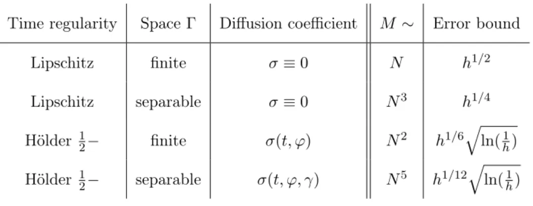
About ten years ago, N. V. Krylov was the first to obtain rates of convergence for finite difference schemes approximating finite-dimensional stochastic control problems with con-trolled and possibly degenerate diffusion matrix, see Krylov (1999, 2000) and the references therein. The error bound obtained there in the special case of a time discretisation scheme with coefficients that are Lipschitz continuous in space and 1₂-Hölder continuous in time is of order h1/6 with h the length of the time step. Notice that in Krylov (1999) the order of convergence is given ash1/3, where the time step has lengthh2. When the space too is discretised, the ratio between time and space step is like h2 againsth or, equivalently, h vs.√h, which explains why the order of convergence is expressed in two different ways.

In Krylov (2005), sharp error bounds are obtained for fully discrete finite difference schemes in a special form; the bounds are of order h1/2 in the mesh size h of the space discretisation and of order τ1/4 _{in the length} _τ _{of the time step.}

Using purely analytic techniques from the theory of viscosity solutions, Barles and Jakobsen (2005, 2007) obtain error bounds for a broad class of finite difference schemes for the approximation of PDEs of Hamilton-Jacobi-Bellman type. In the case of a simple time discretisation scheme, the estimate for the speed of convergence they find is of order h1/10 in the length h of the time step.

A possible ansatz for extending those results to the approximation of control problems with delay is to try to derive a HJB equation for the value function. Recall that a version of the Principle of Dynamic Programming still holds for delay systems, cf. Appendix A.1. As in the finite-dimensional setting, such an HJB equation is not guaranteed to admit classical (i. e. Fréchet-differentiable) solutions, and viscosity solutions have to be defined. The HJB equation can then be used as a starting point for constructing finite difference

4

Generalised solutions for the HJB equation can be shown to exist also in the case when there are no classical solutions, but uniqueness of generalised solutions does not always hold. For viscosity solutions, on the other hand, existence and uniqueness can be guaranteed; moreover, viscosity solutions are the right solutions in the sense that they coincide with the value function of the underlying control problem.

(29)

1.4. AIM AND SCOPE 17

schemes; see Chang et al. (2006) for first results in this direction.

A different approach to the approximation of control problems with delay is to start from a representation of the system dynamics as an evolution equation in Hilbert space. A suitable Hilbert space for this purpose is the space M2 := L2([−r,0],Rd)×Rd, the

Delfour-Mitter space, where r > 0 is the maximal length of the delay. Notice that the segment spaceC([−r,0],Rd)introduced in Section 1.1 can be continuously embedded into

M2. Projection methods could be used to obtain an approximation scheme. For the

representation of controlled deterministic systems with delay, especially linear systems, see Bensoussan et al. (2007: II.4); for how to represent stochastic systems with delay in Hilbert space, see Da Prato and Zabczyk (1992).

A further approach to the discretisation of optimal control problems is based on the Markov property. For a suitable choice of the state space, the controlled processes enjoy the Markov property provided only feedback controls are used as strategies. In the case of problems with delay, the Markov property holds for the segment processes. The dynamics of the original problem are represented by the family of controlled Markov semigroups. Discretisation schemes, especially for time discretisation, can then be studied in terms of convergence of the infinitesimal generators associated with the Markov semigroups; see van Dijk (1984) for an early work. Observe, however, that in order to obtain rates of con-vergence strong regularity hypotheses may be necessary already in the finite-dimensional case; this amounts to assuming that an optimal strategy in feedback form with sufficiently regular (e. g. Lipschitz continuous) feedback function exists or that the value function is two or three times continuously differentiable.

In this work, we will not use any infinite-dimensional representation of the system dy-namics; instead, we will stick to the semi-martingale setting. The Markov property of the (infinite-dimensional) segment processes will nevertheless be exploited. In Section 2.3, we construct approximating discrete-time processes as “extended Markov chains”. In Chap-ter 3, we will make extensive use of a version of the Principle of Dynamic Programming, which is based on the Markov property of the segment processes, cf. Appendix A.1.

Working in the semi-martingale setting has several advantages. Existence and unique-ness results for controlled SDDEs are well-established. There is an elaborate theory charac-terising weak convergence of_Rd-valued semi-martingales (e. g. Jacod and Shiryaev, 1987). This theory will be essential for the convergence analysis of Section 2.3. When the noise process of the dynamics of the original system is a Wiener process – as will be the case in this work –, then the solution processes are Itô diffusions. Strong results on their path regularity, in particular on the moments of their moduli of continuity, are available, cf. Appendix A.2 and Section 3.2. In Section 3.3, we will make use of a finite-dimensional “stochastic mean value theorem” due to N. V. Krylov. The main ingredients in the proof of that result are a mollification trick, the usual PDP and the Itô formula, cf. Theorem A.2 in Appendix A.3.

1.4 Aim and scope

The aim of this thesis is to study discretisation schemes for continuous-time stochastic opti-mal control problems with time delay in the state dynamics. The noise process driving the system of the original control problem will always be a Wiener process – one-dimensional

(30)

in Section 2.3 and multi-dimensional in Chapter 3. The object to be approximated is the value function associated with the original control problem. We are concerned with ques-tions of convergence as well as rates of convergence or bounds on the discretisation error. Error bounds tell how much cannot be lost (or gained) in passing from the original model to a discretised model. This is also the first step in the approximate numerical solution of continuous-time models. For a continuous-time control problem, an approximate numerical solution is usually the only kind of explicit solution available.

The general idea we follow is to replace the original continuous-time control problem by a sequence of approximating discrete-time control problems which are easier to solve numerically. Observe that the value function associated with a continuous-time control problem with delay of the type studied here lives, in general, on a function space, namely the segment space, whence the problem may be considered to be infinite-dimensional.

We will take two approaches. In Chapter 2, we follow the Markov chain method mentioned above, which is a recipe for constructing discretisation schemes and proving convergence in the sense of convergence of associated value functions. In Section 2.1, we present the method as it is found in the work of H. J. Kushner and others. In Section 2.2, we develop an abstract framework in which to state sufficient conditions guaranteeing convergence of approximation schemes. We then apply the method to the discretisation of a class of stochastic optimal control problems with delay and a random time horizon (the time of first exit from a compact set), cf. Section 2.3.

In Chapter 3, we study a more specific scheme, which applies to finite-horizon stochastic control problems with delay, controlled and possibly degenerate diffusion coefficient and multi-dimensional state as well as noise process, cf. Section 3.1. According to the scheme, time and segment space are discretised in two steps, see Sections 3.2 and 3.3. Under quite natural assumptions, we obtain not only convergence, but also bounds on the error of the discretisation scheme, see Section 3.4. The worst-case bound on the discretisation error in the general case is of order nearlyh1/12in the length of the (inner) time step h.

The two-step scheme produces a sequence of approximating finite-dimensional control problems in discrete time. In Section 3.5, we address the question of how to solve these problems numerically. Instead of further discretising the state space – as in Section 2.3 –, we propose to use a variant of “approximate Dynamic Programming”, exploiting the two-step structure of the scheme. Memory requirements, in particular, can be kept at a realistic level.5 Notwithstanding the special structure of the discretisation scheme, its use is not confined to the approximation of finite horizon control problems. It should also apply to systems with a reflecting boundary or systems controlled up to the time of first exit from a compact set.

In this thesis, we are interested in discretisation schemes which yield an approximation to the value function of the original problem. The value function gives thegloballyminimal costs, and knowing it allows to construct globally optimal or nearly optimal strategies (for each initial condition). There are efficient procedures for findinglocally optimal strategies and calculating locally minimal costs, but we will not be concerned with any of them. Moreover, we will not use any hypotheses on the regularity of optimal strategies (not

5

The amount of computer memory required for the two-step scheme depends on the mesh size of the outer time grid. In terms of the length ˜h of this outer time step, a worst-case error bound of order

˜

(31)

1.4. AIM AND SCOPE 19

even existence) nor any regularity assumptions on the value function which are not a consequence of properties of the system coefficients. If such hypotheses were assumed, it would be possible to derive much better rates of convergence. The reason why we refrain from making such assumptions is that they are, usually, difficult or impossible to verify based on the information available about the system to be controlled.

(32)

(33)

Chapter 2

The Markov chain method

There is a general procedure, known as the “Markov chain method” and developed by Harold J. Kushner, for rendering optimal control problems in continuous time accessible to numerical computation. The basic idea is to construct a family of discrete optimal control problems by discretising the original dynamics and the original cost functional in time and space. The important point to establish then is whether the value functions associated with the discrete problems converge to the original value function as the mesh size of the discretisation tends to zero.

If the value functions converge, then the discrete control problems are a valid approxi-mation to the original problem and standard algorithms, notably those based on Dynamic Programming (e. g. Bertsekas, 2005, 2007), can be applied – at least in principle – to cal-culate the minimal costs and to find optimal strategies for each of the discrete control problems.

When the dynamics of the original problem are given by ordinary deterministic or stochastic differential equations, suitable discrete control problems are obtained by re-placing the original controlled differential equations with controlled Markov chains whose transition probabilities are consistent with the original dynamics. Under compactness and continuity assumptions on the original problem, a condition of local consistency for the transition probabilities of the controlled Markov chains suffices to guarantee convergence of the corresponding value functions.

In Section 2.1 we describe the Markov chain method following Kushner and Dupuis (2001) by means of a deterministic example problem. Section 2.2 sets up an abstract frame-work for approximating a given optimal control problem by a sequence of discrete problems. There the continuity and compactness assumptions underlying Kushner’s method are made explicit. In Section 2.3, we apply the method to a class of stochastic control problems with delay and a stopping condition as time horizon. Most of the material of that section has been published in Fischer and Reiß (2007). In Kushner (2005), discretisation schemes for a class of stochastic control problems with delay and reflection are studied; however, the proofs for the delay case do not seem to be as closely analogous to the non-delay case as is suggested there. Section 2.4 contains a brief discussion of the scope of the Markov chain method.

(34)

2.1 Kushner’s approximation method

As an illustration of how Kushner’s method works, let us consider a deterministic opti-mal control problem with finite time horizon. The system dynamics are described by a controlled ordinary differential equation:

(2.1) x˙(t) = b t0+t, x(t), u(t)

, t >0,

where b is a measurable function [0,∞)×Rd×Γ → Rd and u(.) a measurable function

[0,∞)→Γ. The space Γis called the space of control actions and it is assumed thatΓ is a compact metric space. This hypothesis will be crucial later.

The initial state is x(0) = y for some y ∈ Rd. In the formulation adopted here,

solutions x(.) to Equation (2.1) – if there are any – always start at time zero, while the initial time t0 ≥0 enters the equation through the coefficient b. Let Uad be the set of all

Borel measurable functions u : [0,∞) → Γ such that Equation (2.1) possesses a unique absolutely continuous solutionx(.) =xt0,y,u₍_.₎_{for each} ₍_t

0, y)∈[0,∞)×Rd. The elements

ofUad are calledadmissible strategies or, simply,strategies. LetT >0be the deterministic

time horizon. Associated with strategy u ∈ U_ad and initial condition (t0, y) ∈[0, T]×Rd

are the costs

(2.2) Jdet t0, y, u(.) := Z T−t0 0 f t0+t, xt0,y,u(t), u(t) dt + g xt0,y,u₍_T₋_t 0) , where f and g are suitable measurable functions [0,∞)×Rd×Γ → R and Rd → R,

respectively, such that the above integral makes sense as an element of [−∞,∞]. The value function of the control problem determined by (2.1) and (2.2) is given by

Vdet(t0, y) := inf u∈Uad

Jdet t0, y, u(.)

, (t0, y)∈[0, T]×Rd.

The idea is now to construct a suitable family (PM)M∈_N of optimal control problems

in discrete time and with discrete state space so that the corresponding value functions converge pointwise toVdet. The problem PM of degreeM may be obtained as follows. Let

SM ⊂Rd be a regular triangulation of the state spaceRd. Hence, any statey∈Rdcan be

represented as the convex combination of at most d+1 elements ofSM.

The dynamics of the control problem P_M are determined by the choice of a time-inhomogeneous controlled transition function pM:N0×SM ×Γ×SM → [0,1], that is, a

function pM which is jointly measurable and such that pM(n, y, γ, .) defines a probability distribution on SM for all n ∈ N0, y ∈ SM, γ ∈ Γ. Observe that the set SM is at

most countable. The number pM(n, y, γ, z) should be interpreted as the probability that, between time step n and n+ 1, the system switches from state y ∈ SM to state z ∈ SM

under the action of controlγ ∈Γ.

Admissible strategies for the problemPM are adapted sequences(u(n))n∈N0 ofΓ-valued

random variables such that, for each initial condition(n0, y)∈N0×SM, there is an adapted

SM-valued sequence (ξ(n))n∈_N0 whose transition probabilities are given by the function

pM. Strictly speaking, an admissible strategy consists in a (complete) probability space (Ω,F,P)equipped with a filtration(F_n)and an(F_n)-adapted sequence(u(n))ofΓ-valued random variables; thus, the underlying filtered probability space is part of the strategy. For simplicity, we usually omit the stochastic basis from the notation.

Inaugural - Dissertation