Methods to Robust Ranking of Object Trackers and to Tracker Drift Correction

(1)

METHODS TO ROBUST RANKING OF OBJECT

TRACKERS AND TO TRACKER DRIFT CORRECTION

Julien Valognes

A thesis in

The Department of

Electrical and Computer Engineering

Presented in Partial Fulfillment of the Requirements For the Degree of Master of Applied Science in Electrical and

Computer Engineering Concordia University Montr´eal, Qu´ebec, Canada

August 2020

c

(2)

Concordia University

School of Graduate Studies

This is to certify that the thesis prepared

By: Julien Valognes

Entitled: Methods to Robust Ranking of Object Trackers and to

Tracker Drift Correction

and submitted in partial fulfillment of the requirements for the degree of

Master of Applied Science in Electrical and Computer Engineering complies with the regulations of this University and meets the accepted standards with respect to originality and quality.

Signed by the final examining commitee:

Dr. Wei-Ping Zhu Chair

Dr. Thomas Fevens External Examiner

Dr. Wei-Ping Zhu Examiner

Dr. Maria A. Amer Supervisor

Approved by

Dr. Wei-Ping Zhu, Graduate Program Director

2020

Dr. Mourad Debbabi, Interim Dean

(3)

Abstract

Methods to Robust Ranking of Object Trackers and to Tracker Drift

Correction

Julien Valognes

This thesis explores two topics in video object tracking: (1) performance evalua-tion of tracking techniques, and (2) tracker drift detecevalua-tion and correcevalua-tion. Tracking performance evaluation consists into comparing a set of trackers’ performance mea-sures and ranking these trackers based on those meamea-sures. This is often done by computing performance averages over a video sequence and then over the entire test video dataset, consequently resulting in an important loss of statistical information of performance between frames of a video sequence and between the video sequences themselves. This work proposes two methods to evaluate trackers with respect to each other. The first method applies the median absolute deviation (MAD) to effectively analyze the similarities between trackers and iteratively ranks them into groups of similar performances. The second method gains inspiration from the use of robust error norms in anisotropic diffusion for image denoising to perform grouping and ranking of trackers. A total of 20 trackers are scored and ranked across four different benchmarks, and experimental results show that using our scoring evaluation is more robust than using the average over averages.

In the second topic, we explore methods to the detection and correction of tracker drift. Drift detection refers to methods that detect if a tracker is about to drift or has drifted away while following a target object. Drift detection triggers a drift correction mechanism which updates the tracker’s rectangular output bounding box. Most drift

(4)

detection and correction algorithms are called while the target model is updating and are, thus, tracker-dependent. This work proposes a tracker-independent drift detection and correction method. For drift detection, we use a combination of saliency and objectness features to evaluate the likelihood an object exists inside a tracker’s output. Once drift is detected, we run a region proposal network to reinitialize the bounding box output around the target object. Our implementation applied on two state-of-the-art trackers show that our method improves overall tracker performance measures when tested on three benchmarks.

(5)

Acknowledgments

I wish to express my most sincere gratitude to my supervisor, Dr. Maria A. Amer, for her invaluable help in my research, her guidance, and her unwavering patience. This thesis would not have existed in this form had she not believed in me and in my ability to succeed. I have learned and grown significantly from working under her supervision.

I would like to extend my thanks to the members of the VidPro research group for their friendly cooperation and for making the research environment enjoyable.

I also wish to acknowledge my mother, my partner, my in-laws, and my closest friends for their love and their unparalleled support throughout the course of my studies.

(6)

List of Figures

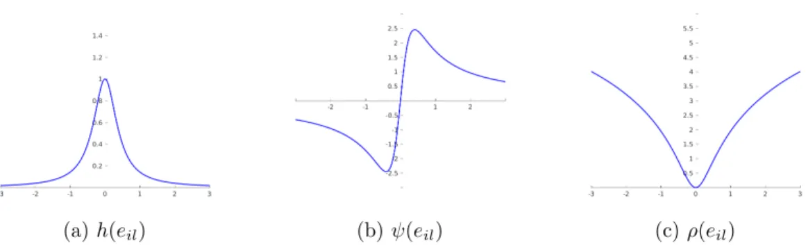
1 Quadratic error normρ(e, σ) and influence ψ(e, σ). . . 40 2 Lorentzian error norm ρ(e, σ) and influence ψ(e, σ). . . 40

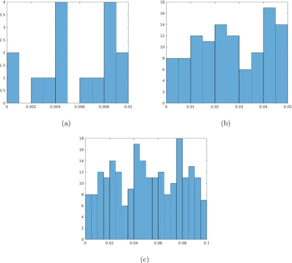
3 Histograms of AOR differences across ranges (a) 0 to 0.01, (b) 0 to

0.05, and (c) 0 to 0.1, in the combined dataset OTB-100+VOT2018-ST+NfS-30. . . 43

4 Perona and Malik edge-stopping function and Lorentzian error norm. 45

5 Huber’s minmax. . . 45 6 Tukey’s biweight. . . 46 7 Histograms of AOR scores {sil} for four categories of trackers: (a)

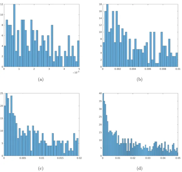
all trackers, (b) lowest category, (c) middle category, and (d) best category, in the combined dataset (i.e., OTB-100+VOT2018-ST+NfS-30). . . 47 8 Histograms of score differences{ηil}across ranges (a) 0 to 0.005, (b) 0

to 0.01, (c) 0 to 0.02, and (d) 0 to 0.05 in the combined dataset (i.e.,

OTB-100+VOT2018-ST+NfS-30). . . 49

9 Histograms of AOR quality data {qil} for three categories of trackers:

(a) lowest category, (b) middle category, and (c) best category, in the

(10)

10 Examples of partial drift (blue) and complete drift (green) from the ground truth (black) in ‘Skydiving’ sequence. . . 70 11 Partitioning of salient regions in sequence ‘gymnastics2’: (a) ground

truth bounding box, and (b) salient segments of the bounding box image. 78 12 Objectness detection in sequence ‘Deer’ with Staple tracker [5]:

Edge-Box proposals (green), StapleBt (black), candidate EB which overlaps

most with Bt (blue), and area AEB (red). . . 79

13 DASIAMRPN (green), our implementation (blue), and ground truth

(black) on ‘Fish2’ sequence of TC128. . . 86

(black) on ‘Badminton1’ sequence of TC128. . . 87

(black) on ‘rabbit’ sequence of VOT2018. . . 87

(black) on ‘soccer2’ sequence of VOT2018. . . 88

(black) on ‘drone1’ sequence of VOT2018. . . 88

(black) on ‘crabs1’ sequence of VOT2018. . . 89

19 SIAMRPN++ (green), our implementation (blue), and ground truth

(black) on ‘Yo-yos2’ sequence of TC128. . . 89

(black) on ‘CarDark’ sequence of TC128. . . 90

(black) on ‘Hand2’ sequence of TC128. . . 90

(11)

23 Failure case: DASIAMRPN (green), our implementation (blue), and ground truth (black) on ‘Kite1’ sequence of TC128. . . 95

24 Failure case: DASIAMRPN (green), our implementation (blue), and

(12)

List of Tables

2 Sequence length information for benchmarks used: number of sequences,

minimum, maximum, average, and total number of frames. . . 6

3 AOR mean ratio, score ratio, and rank difference results under impulse noise and averaged overM = 50 runs for each trackertiin the combined

dataset OTB-100+VOT2018-ST+NfS-30. . . 24

4 AOR mean ratio, score ratio, and rank difference results under

Gaus-sian noise and averaged over M = 50 runs for each tracker ti in the

combined dataset OTB-100+VOT2018-ST+NfS-30. . . 25

5 Percentage of trackers with mean ratio or score ratio above ths. . . . 26

6 Tracking principle and FPS over each benchmark for each tested tracker. 26

7 AOR and FR mean, score, group, and rank for all trackers ti over the

OTB-100 dataset. The 5 top-ranked trackers in terms of AOR are: ECO, LADCF, STRCF, DIMP, CFWCR; those in terms of FR are:

STRCF, LADCF, ECO, DIMP, MDNET. . . 28

VOT2018-ST dataset. The 5 top-ranked trackers in terms of AOR are: DIMP, ATOM, MDNET, SIAMRPN++, IBCCF; those in terms of FR

(13)

NfS-30 dataset. The 5 top-ranked trackers in terms of AOR are: DIMP, ATOM, STRCF, ECO, CFWR; those in terms of FR are: DIMP,

ATOM, CFWCR, ECO, LADCF. . . 30

10 AOR and FR mean, score, group, and rank for all trackers ti over

the combined short-term dataset OTB-100, VOT2018-ST, and NfS-30. The 5 top-ranked trackers in terms of AOR are: DIMP, ATOM, ECO, MDNET, LADCF; those in terms of FR are: DIMP, ATOM, CFWCR, ECO, SIAMRPN++. . . 31 11 AOR and FR mean, score, group, and rank for all trackers ti over the

VOT2018-LT dataset. The 5 top-ranked trackers in terms of AOR are: DIMP, ATOM, DASIAMRPN, SIAMRPN++, LADCF; those in terms

of FR are: DIMP, SIAMRPN++, ATOM, DASIAMRPN, CFWCR. . 33

12 Summarizing results: trackers grouped 1 and trackers ranked 1

(un-derlined and in bold) in all benchmark experiments. . . 33

13 Average AOR per tracker and per sequence and calculated deviation

thresholds dq for best and second best scores, for the OTB-100 dataset. 35

14 AOR mean ratio, score ratio, and rank difference results under impulse noise and averaged overM = 50 runs for each trackertiin the combined

dataset OTB-100+VOT2018-ST+NfS-30. . . 56

15 AOR mean ratio, score ratio, and rank difference results under Gaus-sian noise and averaged over M = 50 runs for each tracker ti in the

combined dataset OTB-100+VOT2018-ST+NfS-30. . . 57

(14)

the OTB-100 dataset. The 5 top-ranked trackers in terms of AOR are: ECO, LADCF, DIMP, ATOM, STRCF; those in terms of FR are:

DIMP, CFWCR, ECO, LADCF, MDNET. . . 59

VOT2018-ST dataset. The 5 top-ranked trackers in terms of AOR are: DIMP, ATOM, MDNET, SIAMRPN++, IBCCF; those in terms of FR

are: DIMP, SIAMRPN++, ATOM, MDNET, CFWCR. . . 60

the NfS-30 dataset. The 5 top-ranked trackers in terms of AOR are: DIMP, ATOM, ECO, CFWCR, LADCF; those in terms of FR are:

DIMP, ATOM, CFWCR, ECO, SIAMRPN++. . . 61

combined short-term dataset OTB-100+VOT2018-ST+NfS-30. The 5 top-ranked trackers in terms of AOR are: DIMP, ATOM, ECO, MD-NET, LADCF; those in terms of FR are: DIMP, ATOM, SIAMRPN++, CFWCR, ECO. . . 62 21 AOR and FR mean, score, group, and rank for all trackers ti over the

VOT2018-LT dataset. The 5 top-ranked trackers in terms of AOR are: DIMP, ATOM, DASIAMRPN, SIAMRPN++, LADCF; those in terms

of FR are: DIMP, SIAMRPN++, ATOM, DASIAMRPN, ECO. . . . 63

22 Summarizing results: trackers grouped 1 and trackers ranked 1

(un-derlined and in bold) in all benchmark experiments. . . 63 23 Top five ranked trackerstibased on the AOR and FR means and scores

(15)

24 Ranks ri of each tracker ti based on the AOR mean, similarity-based

score, and error norm-based score in the combined dataset

OTB-100+VOT2018-ST+NfS-30 and the long-term dataset VOT2018-LT. . . 65

25 VOT2018 and TC128 datasets: Mean FR, AOR, and percentage

im-provement of the RPN-based drift detection and correction over the

original base design of DASIAMRPN and SIAMRPN++. . . 85

26 Selected videos from VOT2018 and TC128: Mean FR, AOR, and

per-centage improvement of the RPN-based drift detection and correction

over the original base design of DASIAMRPN and SIAMRPN++. . . 86

27 VOT2018 and TC128 datasets: Mean FR, AOR, and percentage

im-provement of the RPN-based drift detection and correction over the

(16)

Glossary of Acronyms

AOR Average Overlap Ratio

BB Bounding Box

CF Correlation Filter

CNN Convolutional Neural Network

DC Drift Correction

DD Drift Detection

EAO Expected Average Overlap

EB Edge Box

FPS Frames Per Second

FR Failure Rate

HVS Human Visual System

IoU Intersection over Union

KDE Kernel Density Estimation

LSM Longest Subsequence Measure

MAD Median Absolute Deviation

Pr Precision

RPN Region Proposal Network

RP Region Proposal

Re Recall

(17)

SR Success Rate

TNR True Negative Rate

TPR True Positive Rate

(18)

Chapter 1 Introduction

1.1 Motivation

Visual object tracking has been a growing field of research as it plays a fundamen-tal role in many applications such as activity recognition (e.g., elderly health care or athletes performance measurement), video surveillance, human-computer interac-tions, augmented reality, and robot navigation. Ideally, object tracking techniques aim to follow objects similarly to how the human visual system (HVS) would [14]. Given the initial location of a target object (in the form of a rectangular bounding box) in a video sequence’s first frame, an object tracker aims to estimate the posi-tion of the object in the next frames. While the HVS is well equipped to memorize shapes and anticipate movements in unconstrained environments, developing a ro-bust tracking method which can behave similarly to the HVS remains a challenge due to numerous object-related (scale variation, deformation, motion blur, and fast motion) and environment-related (illumination variation, partial and full occlusion, and background clutter) attributes [48, 91, 55]. Such attributes can lead trackers to show inaccuracies, drift, and potentially fail [17, 18]. Numerous object tracking tech-niques are being continuously presented in the literature to address these challenges

(19)

and one of the central questions is how to evaluate their performance with respect to the state-of-the-art.

In this thesis, we have two main objectives: first, to investigate methods that score and rank trackers and account for how trackers perform with respect to each other; secondly, to investigate methods that detect tracker drift independently of how a baseline tracker is designed. For our first objective, the motivation comes from a recurring problem in object tracking evaluation protocols, which is the evaluation’s reliance on the average as a measure of central tendency for estimating a tracker’s per-formances with respect to other trackers [43, 44, 45, 46, 47, 48, 91, 90, 30, 64, 82, 77]. For our second objective, our motivation comes from the increasing research interest in long-term video tracking challenges, such as drift, failure, or object disappearance [48, 63, 64, 82, 52, 100, 50, 81, 73].

1.2 Problem Statement

Research in video object tracking progresses at such a high rate that many designs are proposed on a yearly basis to compete with the state-of-the-art [48, 63]. One issue that comes with this rapid growth is the difficulty to compare and evaluate as objectively as possible the differences in performances between trackers. Since most rankings are based on averaging averages of performance measures, it has become increasingly difficult to argue which is best between a tracker that performs well in certain sequences but poorly in other sequences, a tracker that fluctuates a lot in-between sequences, and a tracker that performs consistently but slightly less well on average. While ranking according to an average performance measure allows to nu-merically order trackers with respect to each other, minor differences in performance (for example an average difference of 0.03) should not justify alone such ranking. Therefore, it is useful to present a method for scoring and ranking of trackers using

(20)

a robust estimator against outliers.

To this day, developing a tracking algorithm that is robust remains a challenge. Due to appearance changes caused by illumination variation, object deformation, and dynamic motion, it is a complex task for an object tracker to consistently estimate the position of its target object without drifting away. To correct errors caused by tracker drift and prevent a tracker from failing, integrating methods that aim to propose regions in an image (called region proposal networks) may help improve a tracker’s robustness.

1.3 Summary of Contributions

The two main objectives of this thesis are: (1) proposing a scoring and ranking method for evaluation of video object trackers taking into account variations of performance across video frames and across test video sequences, and (2) handling detection and correction of tracker drift by integrating modern region proposal networks .

For our first objective, we divide our contribution into two separate works. Our first work introduces a strategy to effectively determine similarly performing trackers and iteratively rank them by using the median absolute deviation (MAD). Our second work borrows the use of robust error norms in image denoising to propose a robust method for scoring, grouping, and ranking trackers. We show that our scores are more robust to noise and more representative of a tracker’s performance than the widely used average of averages. We consider this robust method as our main contribution in this thesis.

For our second objective, we integrate a tracker-independent drift detection method using both saliency and objectness measures and a drift correction strategy that im-proves the overall robustness of tracking algorithms using region proposal networks.

(21)

1.4 Object Tracking: State-of-the-art

Due to numerous and unpredictable challenges present in video sequences (illumi-nation variation, scale variation, occlusion, deformation, motion blur, fast motion, in-plane rotation, out-of-plane rotation, out-of-view, background clutter, and low res-olution), it is demanding for a tracker to follow any kind of arbitrary target. Over the last decade, object tracking techniques have received lots of attention and have made considerable progress to overcome those challenges.

CNN (Convolutional Neural Network) and CF (Correlation Filter)-based track-ers have significantly advanced the field of visual object tracking and are amidst the state-of-the-art [47, 48, 63]. CF-based visual tracking approaches have attracted con-siderable attention due to being computationally efficient in the Fourier domain and not requiring multiple target appearances. These methods circularly shift versions of the input and regress them to soft class labels. The target object is tracked in the next frame by matching the filter to the search window which yields the highest correlation with the initial object. There exist multiple CF optimization methods to model the input, including sum-of-squared error [8], kernelized correlation filters [40], multiple dimensional features [93], spatio-temporal regularization [53], short-term and long-term memory storage [41], multi-scale estimation [26], CNN-features [54], and patch reliability [57]. CNN-based tracking is another widely applied tracking technique for modeling target appearances on-line. When pre-trained on a large-scale comprehensive dataset, those architectures have shown to carry out significant performance improvements. Discriminative models [65, 38] are off-line pre-trained frameworks which aim to learn a classifier that discriminates a target from its back-ground. Deep regression models [79, 87, 39] more typically integrate CNN features with the discriminative correlation filter framework to predict a set of interdependent values: the bounding box (BB) coordinates in the case of visual tracking. In addition to those two deep-tracking techniques, the Siamese architecture [52, 6, 100, 24, 97]

(22)

has started to gain more attention due to its balance between accuracy and speed. It consists of a CNN applied on two streams, processing the input image and an image patch containing the object of interest separately, and cross-correlates them to search for the test image in the next frame. To this day, most research attention goes to Siamese architectures.

1.5 Datasets and Performance Measures

In this section, we introduce performance measures and datasets which are widely used in video object tracking.

1.5.1 Datasets

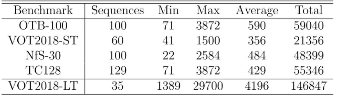
Widely used publicly available benchmarks are OTB-100 [91] (also denoted OTB), VOT2018-ST [48] (also denoted VOT-ST), NfS-30 [42] (also denoted NfS), TC128 [58], and VOT2018-LT [48] (also denoted VOT-LT). These benchmarks are summarized in Table 2.

Each benchmark is compiled for a different purpose. OTB-100 is the first large benchmark introduced to cover all challenging aspects in visual tracking. VOT2018-ST and VOT2018-LT both come from the 2018 VOT challenge [48] but are differen-tiated to tackle short-term and long-term video challenges, respectively. Sequences from the NfS dataset are captured at different frame rates, one at 30 frames per sec-ond (NfS-30) and the other at 240 frames per secsec-ond (NfS-240), to test the impact of frame rate on different tracking architectures. TC128 only contains color sequences in order to understand the role color information has on visual tracking.

Often, trackers perform differently for different datasets. To test the generalization ability of a method, datasets can be combined into one dataset, e.g., one can combine the short-term datasets into a single one called the OTB-100+VOT2018-ST+NfS-30

(23)

Table 2: Sequence length information for benchmarks used: number of sequences, minimum, maximum, average, and total number of frames.

Benchmark

Sequences

Min

Max

Average

Total

OTB-100

100

71 3872

590 59040

VOT2018-ST

60

41 1500

356 21356

NfS-30

100

22 2584

484 48399

TC128

129

71 3872

429 55346

VOT2018-LT

35 1389

29700

4196

146847

dataset.

1.5.2 Performance Measures

To measure performance of object tracking algorithms, we assume there are T track-ers {ti, i = 1,· · · , T} and L test video sequences vl, l = 1,· · ·, L} each having Nl

frames {Ft, t = 1,· · · , Nl}. The objective measures widely used for accuracy and

robustness are Average Overlap Ratio (AOR) and Failure Rate (FR), respectively. OTB-100 [91] and VOT2018 [48] benchmarks make use of said measures, but other benchmarks present variations of them, such as Expected Average Overlap (EAO), Longest Subsequence Measure (LSM), and F-measure (F).

1.5.2.1 Average Overlap Ratio

The AOR measures how accurately a tracker BB is placed with respect to the ground truth over a sequence l. Given vl of Nl frames, it is defined as

AORl = PNl t=1IoUtl Nl ; AOR = PL l=1AORl L , (1)

where AOR is calculated over all L test videos of a dataset, and IoUtl is the ratio

of the number of overlapping pixels (intersection) between the output BB and the ground truth BB and the total number of pixels in the ground truth box of frame Ft

(24)

1.5.2.2 Failure Rate

The FR evaluates the rate at which a tracker completely fails in a video sequence l, i.e., how often IoUtl = 0. Given the Heaviside step function H(.), FR over sequence

l can be written as FRl = PNl t=1H(IoUtl) Nl ; FR = PL l=1FRl L . (2)

This measure may also be used alternatively as the Success Rate SR, where SR =

1−F R, to generate success plots as in [91].

1.5.2.3 Expected Average Overlap

The EAO is an objective measure used in the VOT2018 challenge [49] which combines accuracy values of fragmented sequences to yield an expected AOR value. The VOT protocol re-initializes a tracker after each failure. Any time a tracker fails at frame

Ft of a video sequence l, it is reinitialized to the ground truth BB at the subsequent

frame Ft+5. A sequence vl is thus turned into m+ 1 video fragments if it fails m

times, m ≥ 1. For a tracker i, the VOT challenge calculates EAO as follows. AOR is first measured over the entire video fragments on all frame ranges [1, n], where

n = 2,· · · , Nmax and Nmax is the maximum length of all tested fragments, meaning

evaluated ranges are [1,2],[1,3],· · · ,[1, Nmax]. Only fragments that end with a failure

are picked; the rest is discarded. If a fragment is too short on [1, n], it is padded with zeros. Otherwise, it is trimmed to fit said range. A EAO curve is then obtained by averaging the AOR over all the fragments for each range. Obtaining the desired EAO output consists in averaging the curve in a specific interval H = [Hlow, Hhigh]. To

find H, the authors apply a data smoothing probabilistic Kernel Density Estimation (KDE) model on the dataset {vl}. Hlow and Hhigh correspond to the lengths where

the area under the probability density function is 0.5 and where p(Hlow)≈ p(Hhigh)

(25)

over H is calculated as EAO = 1 Nhigh−Nlow+ 1 Nhigh X n=Nlow EAOn. (3)

In VOT2018-ST, the authors calculate EAO assuming that once a tracker fails, it will keep failing and will not recover. This is not accurate since a tracker may still recover once it has drifted or failed; therefore, we do not use the EAO for evaluation in this chapter.

1.5.2.4 Longest Subsequence Measure

LSM is proposed in [64] to appropriately quantify BB overlap evaluation on long-term tracking rather than short-term. Given the longest successfully tracked subsequence

vλ of a video sequence vl, it is defined as the ratio of the length Nλ of vλ to the full

length Nl of vl. For a tracker i, vλ is a successfully tracked subsequence if x% of

frames Ft in subsequenceλ yield IoUtl ≥0.5. Therefore,

LSMl =

Nλ

Nl

. (4)

The parameter xis a tolerance threshold which the authors set to 95% to allow some tracking failure. This means LSM permits temporary drift or failure to happen but still penalizes cases in which a tracker accidentally recovers a lost target.

1.5.2.5 Precision, Recall, F-measure

These three measures are used in the VOT2018-LT [48] challenge for long-term track-ing evaluation. Trackers in that challenge are required to perform re-detection after a target object is lost. In fact, Precision Pr measures the percentage of all the re-detection predictions (e.g., the tracker BBs) that agree with the ground truth, while Recall Re is the percentage of all the ground truths that agree with the predictions. Widely-used in binary classification, the F-measure provides a Pr/Re trade-off and is

(26)

calculated as follows

F = 2Pr.Re

Pr + Re, . (5)

1.6 Thesis Outline

In Chapter 2, we propose a similarity-based strategy to robustly evaluate and iter-atively rank tested trackers. We employ the median absolute deviation (MAD) to effectively analyze the similarities amidst trackers, place them in groups of similar performance, and rank them to determine which are the top performing trackers.

In Chapter 3, we gain inspiration from image denoising and use the notion of robust error norms in robust statistics to provide a scoring and ranking method that is scientifically solid.

In Chapter 4, we present a drift detection strategy which computes edge-based objectness and superpixel saliency measures on the output bounding box of a tracker. Then, if drift is assumed, a drift correction algorithm relocates the bounding box on the target object using a region proposal network.

In Chapter 5, we summarize our contributions and present future work to conclude the thesis.

(27)

Chapter 2 Similarity-Based Scoring and

Iterative Ranking of Object

Trackers

2.1 Introduction

Each year, numerous tracking techniques are introduced and compete with the state-of-the-art. It is, therefore, important to have a systematic robust ranking strategy for a fair evaluation and comparison of trackers. In the past 20 years, several benchmarks such as CAVIAR [28], CDC [34], FERET [71], iLIDS [3], PETS [2], and MOT [78] became publicly available to encourage research initiatives in video object tracking. Tested trackers are initialized at a single frame of a video sequence with a rectangular-shaped BB and are required to follow an object given that single example. More recent benchmarks [43, 44, 45, 46, 47, 48, 63, 90, 91, 77] also tackle the problem of formulating tracking performances in a manner that is easily quantifiable and as unbiased as possible. The most commonly used indicators for evaluation are tracking accuracy and robustness. However, quantifying accuracy and robustness often requires to measure

(28)

averages over a sequence and then over the entire dataset, consequently resulting in an important loss of statistical information. The final result is, thus, not truly indicative of a tracker’s performance through time, which makes it difficult to evaluate it relatively to that of its counterparts.

This chapter presents our strategy to robustly evaluate and iteratively rank tested trackers; we use the median absolute deviation (MAD) to effectively analyze the similarities amidst trackers while quantifying tracking performances over four bench-marks.

In the rest of this chapter, section 2.2 presents related tracker ranking work; section 2.3 proposes our ranking method; section 2.4 gives simulation results; and section 2.5 concludes the chapter.

2.2 Related Work

Prior related work can be divided into evaluation and ranking of tracking algorithms. Evaluation consists into comparing a set of trackers’ average performance measures [43, 44, 45, 46, 47, 48, 91, 90, 30, 64, 82, 77], while ranking categorizes them based on said evaluation [43, 44, 45, 46, 47, 48, 30, 77, 83, 68].

2.2.1 Evaluation

A variety of datasets are available with their own proposed evaluation methods. Among the most widely-used benchmarks for tracking, OTB-100 [91] consists of 100 short sequences and evaluates trackers using precision and success plots as well as accuracy and robustness measures. Accuracy is measured by the commonly used Av-erage Overlap Ratio (AOR) between a tracker’s BB and the ground truth BB over all test videos, whereas robustness is measured using either Temporal Robustness Evaluation (TRE) or Spatial Robustness Evaluation (SRE). For a given sequence,

(29)

TRE averages all AORs obtained from running a tracker at different frames of the sequence; the tracker is first initialized at the starting frame, and it is then reset to all the consecutive subsequent frames. To measure SRE, the target BB is shifted by 10% of the target size and scaled from 80% to 120% of the ground truth BB. SRE is thus the AOR average of 12 configurations: four center shifts, four corner shifts, and four scale variations. The more recent VOT2018 competition [48] uses a dataset of 60 short sequences and 35 long sequences and is divided into three challenges: short-term, real-time, and long-term. In the short-term VOT2018-ST challenge, three primary measures are applied for tracking evaluation: accuracy, robustness, and Expected Av-erage Overlap (EAO), and trackers which fail are reset to the ground truth five frames later. Under that protocol, robustness simply consists in the number of failures in a video sequence, accuracy is the widely-used AOR, and EAO, which is introduced to account for variable sequence lengths, estimates the AOR a tracker is expected to yield on a dataset of equally sized short sequences. The real-time challenge works similarly to the short-term one but adds a constraint on tracking speed; tested track-ers require to run at a speed equal or greater to 20 frames per second (FPS), and trackers that do not respond in time are penalized by assigning their last reported BB for evaluation. For long-term tracking, however, the VOT2018-LT challenge uses precision Pr, recall Re, and a standard tracking F-score as per [62] to combine Pr with Re and optimize their tradeoff. [77] covers various video tracking challenges in 315 sequence fragments and also combines precision Pr and recall Re using an overlap-based F-score with a 50% Intersection over Union (IoU) criterion to distinguish false positives from true positives.

Most available datasets for tracking evaluation have been tailored for short-term scenarios, which are not representative of real life applications. To address such disparity, researchers have proposed more largely scaled tracking benchmarks. The VOT challenge [48], for instance, had only started introducing long-term tracking

(30)

evaluation in 2018. [64] introduces its own TLP dataset of 50 lengthy videos of approximately 13500 frames each on average. The authors also divide this benchmark into two other separate datasets: TinyTLP, which consists of each sequence’s first 600 frames to match the OTB-100 dataset average length, and TLPattr, which comprises of 90 short sequences categorized on a challenge basis (fast motion, illumination variation, scale variation, partial occlusion, out-of-view or full occlusion, background clutter). [64] proposes the Longest Subsequence Measure (LSM) objective measure to address a tracker’s ability to continuously track a target in lengthy videos and with a certain tolerance for failure. [82] focuses on the problem of target re-detection due to objects not always being present throughout segments of video sequences. The authors evaluate object localization by calculating the geometric mean of the True Positive Rate (TPR) and True Negative Rate (TNR) of the estimated object presence at each frame. This measure differs from the more commonly applied ones for robustness as it evaluates more a tracker’s ability to re-detect an object in long sequences rather than its ability to recover from occurring drift.

2.2.2 Ranking

The authors in [43, 44, 45, 46, 47, 48] evaluate all tested trackers based on accuracy and robustness measures and numerically rank them from best to worst. VOT2013 [43] includes three experiments: firstly with initialization on the ground truth BB, secondly with initialization on a noisy ground truth BB, and lastly with gray-scaled image sequences. Trackers are then ordered accordingly to a joint ranking of all three experiments. VOT2014 [44] does a joint ranking of only the two first experiments, leaving the gray-scaled one behind. Compared to the first one, the second experiment adds an element of randomness to the initialization of all trackers by perturbing the size and shape of the ground truth BB up to 10%. [45] introduces the first VOT-TIR in 2015 to rank trackers in infra-red and thermal imagery. The authors also add the

(31)

EAO performance measure to which the ranking is based, and the following VOT2016 challenge [46] follows that protocol as well. The 2017 VOT challenge [47] evaluates and ranks similarly to the previous one but adds a real-time challenge which accounts for tracking speed in the ranking process. The 2018 VOT challenge [48] tackles three experiments separately, short-term, real-time, and long-term tracking, to which each have their own ranking. Finally, the VOT 2019 challenge [63] adds two challenges: VOT-RGBT, which focuses on short-term tracking in RGB and thermal imagery, and VOT-RGBD, which focuses on long-term tracking in RGB and depth imagery. [4] revisits the VOT 2013 challenge alongside OTB-100 and creates mirror-transformed versions of these datasets to evaluate and rank the robustness of trackers subject to mirroring.

In [83], the authors conduct a comparative experiment on several objective mea-sures to determine which are equivalent information-wise and then rank a set of test trackers using the least correlated measures to reflect on different aspects of tracking. Similarly, [77] searches for multiple measures to best describe accuracy and robust-ness but its final decision on which measures to use for ranking is biased from the start as it favors detection-based trackers. [42] compares accuracy and real-time per-formances on a dataset at two different frame rates (30 FPS and 240 FPS) and shows that changing the frame rate affects the ranking of trackers depending on their track-ing principle. [68] applies four different ranktrack-ing methods and averages them into a mean rank; the first two model datasets as graphs and assign ranks using both an aggregation algorithm and a PageRank-based solution [67], whilst the two last rank-ings are derived from the Elo [22] and Glicko [33] sports rating systems. Similarly to our work, the authors of that paper identify trackers as either best or second best; however, any tracker which is not qualified as best is automatically assumed to be second best, whereas our algorithm objectively justifies both score assignments.

(32)

2.3 Proposed Ranking Method

Our proposed method consists of three stages: scoring, grouping, and ranking. The inputs to the system are (a) the output BB of all tested trackers {ti;i = 1,· · ·, T}

over all the test sequences {vl;l = 1,· · ·, L}, each sequence has Nl frames {Ft;t =

1,· · · , Nl} (b) the ground truth BBs over said sequences, (c) the performance

mea-sure, and (d) the data dispersion estimator, MAD (Median Absolute Deviation) in our case. Quality data qil is first calculated according to the selected measure (for

example, AOR or FR) over each tracker i and sequence l. The scoring stage applies the data dispersion estimator on each T-sized row of {qil} and outputs a score si to

each ti; _L1 ≤ si ≤ 1. A higher si for a tracker i indicates that ti is more consistent

in yielding good outputs. The output vector {si} serves as the input quality data

for the grouping and ranking stages where, again, the MAD dispersion estimator is iteratively applied on {si}to group all trackers i into groups {gi} and ranks {ri}.

2.3.1 Similarity-Based Scoring

The input to scoring is a T byL matrix of quality data{qil}. A trackerti scores best

or second best when it achieves best or second best average performance among the entirety ofT trackers for a sequencel. However, due to possible outliers or similarities in the quality data for a vl, simply appointing the best and second best scores to the

two top performance values does not make up for a fair assignment, as doing so does not account for the dispersion in the quality data. We, therefore, define for each test sequence l a deviation threshold dq based on the MAD estimator as in (6),

dq =M edian(|{qil} −M edian({qil})|). (6)

For each tracker i, the MAD evaluates its quality data’s affiliation to either a best or a second best score. Our scoring methodology is described in Algorithm 1 and is ran twice to first assign best scores, then second best scores. Scores are appointed to

(33)

trackers{ti}on a per-sequence basis until all sequences{vl}are processed sequentially.

For each ti and an objective measure, the final score si over all {vl}is the normalized

summation of all its obtained scores for that measure; therefore, the output is a set of T final scores. In the first scoring round, all trackers i are scored, whereas in the second round, only trackers which have not scored best are considered for evaluation. In Algorithm 1,Best({qil}) represents the best value (for instance the maximum AOR

or the minimum FR) in a set {qil}.

Algorithm 1: Scoring of trackers over all {vl}for an objective measure.

Data: Quality data {qil} of all trackers {ti;i= 1,· · · , T} on all test

sequences{vl;l = 1,· · · , L}.

Result: Scoresi for each ti.

1 for each tracker t_i do

2 si = 0;

3 end

4 for each test sequence v_l do 5 dq =M AD({qil});

6 q_o =Best({q_il}); 7 for each tracker t_i do 8 if |qil−qo|< dq then 9 s_i =s_i+ 1; 10 end 11 end 12 end 13 {si}= {s_Li};

Since a ti can be given either a best or a second best score, more weight is

at-tributed to the best ones. Therefore, we set the score weighting system{best, second best} to fixed values {0.8,0.2}. We also altered those weights from 0.6 to 0.9, with increments of 0.1, and did not notice important variations in our final scoring results when compared to our chosen distribution. We also thought about increasing the number of best sets of scores to evaluate; however, increasing the number of best sets does not improve our system and is even more likely to assign a score to trackers that are poorly performing. In the scenario where we would have added a third best

(34)

score, the weight would be so low that the final output would not be too different to our current scoring system. For this reason, we only score best and second best performing trackers.

2.3.2 Similarity-Based Grouping

Grouping divides the T test trackers into a set of groups {gi, i = 1,· · · , G ≤ T} of

similarly performing trackers based on theT scores{si} of an objective measure over

all test sequences {vl}. We name group the ti which share similar gi. There can be

T groups if all trackers have fully different scores; otherwise, the number of groups

G < T.

Algorithm 2 shows how grouping is performed. First, it calculates the MAD threshold ds over the T scores si of the unassigned (not yet grouped) trackers i

in {ti}. A score si which is within the range defined by ds and max({si}) has its

corresponding tracker assigned a counter count as its group gi; the counter starts

at 1 and increments after each round. A new round of grouping starts if there still exists an unassigned tracker in {ti}. The grouping algorithm ends whenever each ti

is assigned a gi.

Algorithm 2: Grouping of all trackers {ti}.

Data: Scoring data {si} of all trackers {ti;i= 1,· · · , T}.

Result: Groupgi for each ti.

1 count= 1;

2 while ∃ unranked t_i in {t_i} do 3 ds =M AD({si});

4 s_o= max({s_i});

5 for each unassigned t_i in {t_i} do

6 if |si−so| ≤ds then 7 g_i =count; 8 end 9 end 10 count+ +; 11 end

(35)

2.3.3 Iterative Ranking

The T tested trackers are iteratively scored and ranked based on the quality data

{qil} over all test sequences {vl}. At the start of each iteration k, each tracker is

placed in a set j of trackers with the same assigned rank {ti}j, j = 1,· · · , J ≤ T.

Initially, none of the ti are ranked and they all belong in the same set j of unranked

trackers (i.e., r0

i = 0 and J = 1). The first iteration is similar to grouping; therefore,

r1

i =gi. At iteration k, a rank is assigned at each tracker and multiple trackers may

have the same rank. The ranking algorithm ends whenever all ranks in the final set

{r1:k

i } are all distinct from each other or when k =T. For more simplicity, the final

rank obtained at the last iteration is named rank and is noted ri. As an example,

iterations operate as follows. In the first iteration, the ranking algorithm ranks and partitions the T trackers into J1 _sets _j1 _{based on the trackers’ scores} _{_s

i} computed

from the quality values {qil}; best trackers are in set 1, second best trackers are in

set 2, third best trackers are in set 3, etc. In the second iteration, the J1 sets j1 are partitioned intoJ2 _{> J}1 _subsets_j2 _{based on the scores re-computed from the quality}

values {qil}j of the ti in each set j1. Scores are re-computed in each set to better

determine how trackers within the same set perform with respect to each other. In the following iterations, the same process is repeated: subsets are partitioned into smaller subsets, and all trackers in the same newly partitioned subset are scored and ranked against each other. In the last iteration, there can be up to J =T sets, that is, when all trackers are ranked differently.

Algorithm 3 shows more precisely how the entire ranking process is achieved. First, we use the quality data Qj = {qil}j, in other words, the quality values of

trackers i in the set of trackers {ti}j over all test sequences {vl}. Qj is a matrix of

size Tj×L, where Tj =|{ti}j|is the number of trackers in {ti}j at iteration k; a row

in Qj designates a tracker i from{ti}j and a column designates a sequence l. Then,

(36)

2.3.1 to produce theTj scores of setj, namely{si}j. We calculate the MAD threshold

ds over{si}j, and a score which is within the range defined by ds and max({si}j) has

its corresponding tracker assigned a counter count as its rank r_ik; the counter starts at 1 and increments after each round of ranking (“while” loop in Algorithm 3), that is, after at least one tracker in {ti}j has been ranked. A new round starts if there

still exists an unranked ti in {ti}j. Once all trackers are ranked in iteration k, we

take the new sets {ti}j of similarly ranked trackers for iteration k+ 1. The setsj for

iteration k+ 1 depend on the tracker ranks at iterationk, andj varies from 1 and J. The algorithm iterates if k≤T and if at least two trackers are of the same rank. The algorithm stops either when k=T + 1 or when all trackers are ranked differently. In fact,T is the minimal amount of iterations required to fully achieve ranking, without exception, over all {ti}. Hence, a final rank 1 ≤ri ≤ T and only trackers that have

the same score end with the same rank.

Essentially, algorithm 3 in its first iteration k = 1 divides all trackers {ti} into

groups (same as algorithm 2); then, in each of the following iterations, each group is divided into sub-groups, and each tracker in each sub-group is given a rank. Ranking is based on the scores which are recomputed at each iteration. This is repeated until all trackers are ranked.

At each new iteration, each trackers within a same setj have its score recomputed. The score at k = 1 is the most relevant to display for analysis since it is used for grouping and shows how all T trackers compare with respect to the top performing trackers. At the last iteration, the final score of a tracker i is simply the score of the tracker in the last set it was assigned in. This means the final score is not meaningful to show or interpret on its own. However, the final rankri depends on all scores, from

the first iteration to the last iteration, hence the importance of computing scores at each iteration.

(37)

Algorithm 3: Iterative ranking of all trackers {ti}.

Data: Quality data {qil} of all trackers {ti;i= 1,· · · , T} on all test

sequences{vl;l = 1,· · · , L}.

Result: Rankri for each ti.

1 k = 1; 2 j = 1; 3 {t_i}_j ={t_i}; 4 do 5 for each {ti}j do 6 Q_j ={q_il}_j; 7 {s_i}_j =score(Q_j); 8 count= 1; 9 while ∃ unranked t_i in {t_i}_j do 10 d_s =M AD({s_i}_j); 11 so = max({si}j);

12 for each unranked t_i in {t_i}_j do

13 if |s_i−s_o| ≤d_s then 14 rk_i =count; 15 end 16 end 17 count+ +; 18 end 19 end 20 k+ +; 21 {t_i}_j =update({t_i}_j);

(38)

2.3.4 How Robust is our Method?

Our scoring and ranking methods are based on a robust dispersion estimator: the

MAD. To demonstrate their robustness, we run a total of M experiments where the

original AOR quality data of each frame of a test video signal and for all trackers are subjected to variations of signal independent noise; then, we evaluate our algorithm’s response to impulse and non-zero mean Gaussian noise.

In the context of this experiment, impulse noise can be interpreted as the result of random sharp and sudden image changes such as occlusion or fast motion. We can also interpret the additivity of Gaussian noise to {qil} as random gradual changes

through frames such as illumination variation or motion blur.

To show the robustness of our scoring method, given T tested trackers {ti;i =

1,· · · , T}, let their scores be {si} and mean measures be {pi} generated from the

original quality data {qil} of an objective measure (such as AOR) over all sequences

{vl}, and let their noisy scores be {sin} and noisy mean measures be {pni} generated

from the noisy quality data{qn

il}of that same objective measure. Our scoring is more

robust than averaging (mean) if, after M experiments,

∀i, Ψ(si, µsn

i)>Ψ(pi, µp n

i), (7)

where Ψ(·) = _maxmin(₍·_·)₎ ∈[0,· · · ,1] is a min-max ratio applied for normalization,

µsn i = 1 K K X k=1 sk_i, (8) µpn i = 1 K K X k=1 pk_i. (9) µsn

i is the average score of tracker i over K different levels of a noise distribution under test, and µpn

i is the average performance mean of tracker i over the same K noise levels. In other words, our scoring is more robust than the mean if, overall, each

ti yields a ratio of scores Ψ(si, µsn

(39)

To test if our ranking method is robust, let the ranks of all the T trackers be

{ri} generated from the original quality data {qil}of an objective measure over each

sequence l, and let their noisy ranks be {rn_i} generated from the noisy quality data

{qn

il} of that same objective measure. Our ranking is robust if, afterM experiments,

∀i, |ri−µrn

i| ≤1, (10)

where µrn

i is the average rank of each tracker i over K different levels of a noise distribution, µrn_i = 1 K K X k=1 rk_i. (11)

In other words, our ranking is robust if, overall, each ti yields at most a difference of

1 between its original ri and its corresponding average of noisy ranks µrn i.

Given the original overlap ratio quality data {qil}, that is, AORl values at each

test video sequence vl for each tracker ti, we add noise to AORl to get {qnil}. For

im-pulse noise, the noisy quality data{qn

il}is the original quality data to which we apply

a binary-state sequence, with a noise density varying from 0.05 to 0.5, specifically, 0.05, 0.2, 0.35, and 0.5. For Gaussian noise, we pick three distributions with different standard deviations std, namely 0.01, 0.05, and 0.1. To each Gaussian distribution, we vary the mean from 0.1 to 0.4, specifically, 0.1, 0.2, 0.3, and 0.4. We run the

exper-iments M = 50 times across the combined dataset OTB-100+VOT2018-ST+NfS-30.

Tables 3 and 4 display Ψ(pi, µpn

i) (noted ‘Mean ratio’), Ψ(si, µsni) (noted ‘Score ratio’) and |ri −µrn

i| (noted ‘Rank diff.’) results under impulse noise and Gaussian noise, respectively. Both tables show that our proposed ranking responds moderately to even strong variations in the input data not just on average, but for every tracker

i. Indeed, the rank difference is less or equal to 1, affirming the robustness of our ranking methodology. We also see that, overall, the score ratio does not goes below 0.85, which is comparatively much more robust than the mean ratio where the ratio can reach 0.55. We notice that in the case of impulse noise, the average score ratio

(40)

and the average mean ratio are comparable and remain above 0.9, but in all cases of Gaussian disturbances, the score performs much better than the mean.

In Table 5, we show the percentage of trackers with mean ratio and score ratio above a certain thresholdths over all 16 cases of noise levels: 4 levels of impulse noise

as per Table 3 and 12 levels of Gaussian noise as per Table 4. We can observe that the score is more robust than the mean.

We applied our robustness experiment only to the AOR values AORl at each

sequence but not to the FR values FRl because the latter are too small. In fact, the

average of all our AOR data is 0.46331, whereas that of our FR data is 0.2535, and larger levels of noise negatively affects the experiment if our measure is, overall, closer to 0 or to 1 (here the FR). To keep our noise distribution as unaltered as possible, it is best to operate on a measure that is, overall, closer to 0.5 (here the AOR).

2.4 Results and Discussion

2.4.1 Experimental Setup

For testing our methods, we selected 20 trackers of different performance, speed, and with their code publicly available: ATOM [24], CFWCR [38], CREST [79], CSRDCF [61], DASIAMRPN [100], DAT [72], DIMP [97], DLST [94], DSST [26], ECO [25], IBCCF [54], KCF [40], LADCF [92], MCCT [86], MDNET [65], SAMF [93], SIAMFC [6], SIAMRPN++ [51], STAPLE [5], and STRCF [53]. Table 6 briefly describes each of their tracking principles. As can be seen, the majority of them are correlation filter-based, CNN-filter-based, Siamese, or a combination of architectures, as those methods have proven to compete most with the state-of-the-art [47, 48, 63]. DAT was chosen to compete among the older trackers and is the only one to solely rely on a color tracking principle. LADCF and MCCT trackers used in our evaluation are correlation filter-based but also exist with a CNN architecture.

(41)

Table 3: AOR mean ratio, score ratio, and rank difference results under impulse noise and averaged over M = 50 runs for each tracker ti in the combined dataset

OTB-100+VOT2018-ST+NfS-30.

(a) Impulse noise of density 0.05 and 0.2 (b) Impulse noise of density 0.35 and 0.5

(42)

Table 4: AOR mean ratio, score ratio, and rank difference results under Gaussian noise and averaged over M = 50 runs for each tracker ti in the combined dataset

OTB-100+VOT2018-ST+NfS-30.

(a) Gaussian noise with std = 0.01 and means 0.1, 0.2, 0.3, and 0.4

(b) Gaussian noise with std = 0.05 and means 0.1, 0.2, 0.3, and 0.4

(c) Gaussian noise withstd= 0.1 and means 0.1, 0.2, 0.3, and 0.4

(43)

Table 5: Percentage of trackers with mean ratio or score ratio above ths.

Threshold

Mean ratio

Score ratio

th

s

% trackers

0.85

38

72.5

0.9

37

56

0.95

28

Table 6: Tracking principle and FPS over each benchmark for each tested tracker. Tracking Principle Siamese Discriminative CNN Color Code Frames per second Average

Network Correlation Filter Matching Template OTB VOT-ST VOT-LT NfS FPS 1. ATOM [24] X - X - CC / GPU / P 21.324 25.761 30.836 24.468 25.597 2. CFWCR [38] - X X - PC / GPU / M 3.231 4.675 2.890 2.828 3.578 3. CSRDCF [61] - X - - PC / CPU / M 15.008 12.543 10.455 9.993 12.515 4. CREST [79] - X X - PC / GPU / M 1.463 1.592 1.316 1.674 1.576 5. DASIAMRPN [100] X - X - CC / GPU / P 68.313 175.55 71.724 72.341 96.982 6. DAT [72] - - - X PC / CPU / M 90.975 55.100 44.948 43.908 63.328 7. DIMP [97] _X - _X - CC / GPU / P 25.792 26.520 30.438 26.606 27.339 8. DLST [94] - - X - PC / GPU / M 0.888 0.899 - 0.774 0.854 9. DSST [26] - X - - PC / CPU / M 53.054 54.516 39.683 42.193 49.921 10. ECO [25] - X X - PC / GPU / M 2.082 2.298 1.934 1.394 1.925 11. IBCCF [54] - X X - PC / GPU / M 0.660 0.670 0.559 0.572 0.634 12. KCF [40] - X - - PC / CPU / M 121.960 79.050 51.262 37.436 79.482 13. LADCF [92] - X - - PC / CPU / M 23.775 21.853 18.755 19.291 21.640 14. MCCT [86] - X - - PC / CPU / M 39.094 7.476 27.665 32.696 26.422 15. MDNET [65] - - X - PC / GPU / M 0.708 0.717 0.641 0.659 0.695 16. SAMF [93] - X - - PC / CPU / M 26.185 15.031 8.636 6.502 15.906 17. SIAMFC [6] X - X - PC / GPU / M 14.117 13.93 - 8.919 12.322 18. SIAMRPN++ [51] _X - _X - CC / GPU / P 47.747 44.494 30.973 39.464 40.670 19. STAPLE [5] - X - - PC / CPU / M 77.335 71.463 49.510 61.56 70.119 20. STRCF [53] - X - - PC / CPU / M 25.985 20.568 18.001 18.935 21.829

(44)

We collect the mean, score, group, and rank of each tracker for AOR and FR measures over three short-term datasets: OTB-100 [91], VOT2018-ST [48], and NfS-30 [42] (Chapter 1 section 1.5.1 briefly introduces these datasets). The scores and groups displayed in all following tables is that calculated at iterationk = 1 since that is the only time all trackers compete against each other.

2.4.2 Experimentation on OTB-100 Dataset

Mean, score, group, and rank results over the 100 sequences of OTB-100 are displayed in Table 7. We first notice that the scoring does not replicate outputs similar to the mean. For example, there is much more variance in the AOR scores of DIMP and ECO trackers than in their respective mean AOR. We also see that a tracker can score higher even if it has a lower mean than another tracker. For example, DASIAMRPN has a higher mean AOR than CSRDCF but its score is slightly lower. Our results show that the score does not directly correlate with the objective measure itself; it is instead an indication of the frequency at which a tracker performs best relatively to its counterparts using that objective measure. Hence, ranking would be different if it were done according to the mean. Table 7 also shows that one tracker can be overall more accurate (i.e., higher AOR score) than another one, while being simultaneously less robust (i.e., lower FR score). For instance, SIAMRPN++ is in groups 5 and 2 for AOR and FR, respectively, whereas STAPLE is assigned groups 3 and 3 for those measures. This means that SIAMRPN++ overall fails less than STAPLE on OTB-100, but that STAPLE more consistently yields better accuracy. Moreover, we notice less differences between FR scores and means than between AOR scores and means. This makes sense since many of our tested trackers rarely fail and yield consistent FR results across the widely studied OTB-100 dataset. Consequently, FR data variability is much lower and the ranking based on score looks more closely to that which would be based on the mean.

(45)

Table 7: AOR and FR mean, score, group, and rank for all trackers ti over the

OTB-100 dataset. The 5 top-ranked trackers in terms of AOR are: ECO, LADCF, STRCF, DIMP, CFWCR; those in terms of FR are: STRCF, LADCF, ECO, DIMP, MDNET.

AOR results split the trackers into 7 groups of performance. The first AOR group includes ATOM, CFWCR, DIMP, ECO, LADCF, and STRCF. FR results split the trackers into 5 groups which is a smaller amount of groups than with AOR. The first FR group includes ATOM, CFWCR, DIMP, ECO, LADCF, MDNET, and STRCF trackers, which is one more tracker than the first AOR group. In fact, the lower data variability in FR explains the reduced number of groups, hence the addition of MDNET in group 1.

2.4.3 Experimentation on VOT2018-ST Dataset

Mean, score, group, and rank results over the 60 sequences of VOT2018-ST are dis-played in Table 8. For matters of consistency with OTB-100, we use a rectangular annotated ground truth at each frame instead of the rotated one provided by the benchmark. We first notice that the number of AOR and FR groups are larger than in OTB-100, underlying the higher dispersion of data. In addition to that, the mean

(46)

VOT2018-ST dataset. The 5 top-ranked trackers in terms of AOR are: DIMP, ATOM, MDNET, SIAMRPN++, IBCCF; those in terms of FR are: DIMP, SIAMRPN++, MDNET, ATOM, CSRDCF.

performance measures are lower overall than in OTB-100. Despite having shorter sequences on average, VOT2018-ST has more challenging videos than OTB-100, and such attributes increase a tracker’s likeliness to drift earlier in a sequence. Indeed, datasets from the VOT challenge are updated to keep up with the state-of-the-art, whereas OTB-100 has remained unchanged since its release.

AOR and FR performance measures divide the candidate trackers into 8 and 6 groups, respectively. AOR group 1 only consists of DIMP whereas FR group 1 includes DIMP, MDNET, and SIAMRPN++. Trackers such as ATOM, ECO, and LADCF that were ranked first in Table 7 over OTB-100 are now ranked in a lower group, hence emphasizing the difference in performance between those trackers and DIMP.

(47)

Table 9: AOR and FR mean, score, group, and rank for all trackersti over the NfS-30

dataset. The 5 top-ranked trackers in terms of AOR are: DIMP, ATOM, STRCF, ECO, CFWR; those in terms of FR are: DIMP, ATOM, CFWCR, ECO, LADCF.

2.4.4 Experimentation on NfS-30 Dataset

The NfS benchmark is not as well known or as widely used as OTB-100 and VOT2018-ST. It is divided into two datasets of 100 video sequences captured at different frame rates: 240 FPS (NfS-240) and 30 FPS (NfS-30). All frames are annotated with a rectangular ground truth. We test the trackers on NfS-30 as it presents a variety of examples which have not been explored as much as in OTB-100 and VOT2018-ST datasets, thus allowing to test their robustness to different target objects and envi-ronments. Table 9 displays AOR and FR performance results over the 100 sequences. AOR and FR results split the trackers into 8 and 7 groups of performance, re-spectively. The FR-based number of groups is the highest amount among the three studied datasets. This means there is more FR variance in the NfS-30 than in the other datasets. Trackers ranked in the first group for both AOR and FR measures are ATOM and DIMP. Trackers such as ECO, LADCF, and MDNET which have ranked high in either OTB-100 or VOT2018-ST are placed in groups 2 or 3.

(48)

combined short-term dataset OTB-100, VOT2018-ST, and NfS-30. The 5 top-ranked trackers in terms of AOR are: DIMP, ATOM, ECO, MDNET, LADCF; those in terms of FR are: DIMP, ATOM, CFWCR, ECO, SIAMRPN++.

2.4.5 Experimentation on Cross Datasets (Short-Term)

To obtain an overall evaluation of each tracker’s accuracy and robustness performance across all short-term datasets (OTB-100, VOT218-ST, and NfS-30), one method would be to collect the rank of each tracker in each dataset and then assign it the mean or median rank as its final rank. Doing so, however, poses certain issues: (1) two different trackers may be assigned a similar final rank, hence defeating the purpose of ordering them, (2) smaller datasets are treated as equally as larger datasets, and (3) some trackers are trained to perform better in a specific benchmark, therefore, affecting the ranking when performed on that benchmark. To reduce possible bias towards certain benchmarks, test the generalization ability of the trackers, and make the ranking more fair, we run the scoring and ranking across all 260 video sequences of OTB-100, VOT2018-ST, and NfS-30 combined. In doing so, the output of our scoring and ranking method is a set of ranks and groups assigned at each tracker.

(49)

Table 10 displays AOR and FR means, scores, ranks, and groups across the com-bined short-term dataset. There is a total of 7 groups for AOR and 6 groups for FR. We see that ATOM and DIMP trackers are in group 1 for both AOR and FR performance measures. In addition, CFWCR, ECO, LADCF, MDNET, and STRCF trackers are in group 2 for both AOR and FR measures are. Even though CFWCR, ECO, LADCF, and STRCF were top trackers in OTB-100, we can clearly see that ATOM and DIMP are the best performing ones on the cross datasets.

2.4.6 Experimentation on Long-Term Dataset VOT2018-LT

We run the scoring and ranking on the VOT2018-LT dataset, consisting of 35 long-term videos. The aim of this experiment is to observe how much tracking perfor-mances can be affected by video length and differ from those on short-term videos. AOR and FR means, scores, ranks, and groups are displayed in Table 11.

We notice that DIMP is the only tracker to be assigned group 1 on both AOR and FR measures since it performs, overall, much better than its counterparts. Nonethe-less, we can observe that ATOM, DASIAMRPN, LADCF, and SIAMRPN++ are in group 2 for both measures; among those four trackers, three of them (ATOM, DASIAMRPN, and SIAMRPN++) have an implemented target re-detection algo-rithm which allows them to reduce error loss when facing long-term challenges. While trackers such as ECO, MDNET, and STRCF performed well on short-term sequences, their incapability to re-detect lost objects puts them at a disadvantage on long-term sequences.

(50)

VOT2018-LT dataset. The 5 top-ranked trackers in terms of AOR are: DIMP,

ATOM, DASIAMRPN, SIAMRPN++, LADCF; those in terms of FR are: DIMP, SIAMRPN++, ATOM, DASIAMRPN, CFWCR.

Table 12: Summarizing results: trackers grouped 1 and trackers ranked 1 (underlined and in bold) in all benchmark experiments.

Dataset AOR FR

OTB ECO, LADCF, STRCF, DIMP, CFWCR, ATOM STRCF, LADCF, ECO, DIMP, MDNET, CFWCR, ATOM

VOT-ST DIMP DIMP, SIAMRPN++, MDNET

NfS DIMP, ATOM DIMP, ATOM

VOT-LT DIMP DIMP

OTB+VOT-ST+NfS DIMP, ATOM DIMP, ATOM

2.4.7 Analysis and Discussion

2.4.7.1 Which are the Best Performing Trackers?

We summarize in Table 12 which trackers achieve rank 1 (i.e., ri = 1) at the end

of our iterative algorithm and which ones achieve group 1 (i.e., r1

i = 1) after the

first iteration. We see that ECO, DIMP, MDNET, and STRCF achieve rank 1 in either accuracy or robustness, and that ATOM, CFWCR, ECO, DIMP, LADCF, and MDNET achieve group 1 for both AOR and FR, simultaneously, across at least one dataset. When all three short-term datasets are merged, ATOM and DIMP are placed in group 1, and DIMP is ranked 1 for both AOR and FR.

(51)

ATOM and DIMP ranks are also preserved when looking into the four individual experiments (OTB-100, VOT2018-ST, NfS-30, and VOT2018-LT). By counting how often a tracker achieves group 1 in AOR and FR measures across all four benchmarks, we see that DIMP scores 8/8, followed by ATOM with 4/8, then CFWCR, ECO, LADCF, MDNET, and STRCF with 2/8, and finally SIAMRPN++ with 1/8.

Table 12 confirms that deep-learning trackers (here ATOM and DIMP), correlation filter-based trackers (here LADCF and STRCF), or a combination of both tracking principles (here CFWCR and ECO) well compete against each other. We also note from Table 6 that the fastest of those top trackers are ATOM and DIMP, each running at 25.6 and 27.3 FPS, respectively. Overall, the top tracker in our benchmark is DIMP.

2.4.7.2 Detailed Output of Proposed Algorithm

In the proposed algorithm, each tested trackeriis evaluated over each video sequence

l to yield scores {si}. We calculate the MAD threshold on two rounds to filter out

top performing and second top performing trackers from the rest of {ti}. Table 13

illustrates how our scoring algorithm works, where the performance measure is AOR, and all test sequences with their calculated MAD thresholdsdq (denoted thresh1 and

thresh2 in Table 13) for best and second best scoring are displayed.

2.5 Conclusion

Numerous trackers are proposed yearly and compete with the state-of-the-art; our goal in this study was to identify trackers which were of similar AOR and FR performances across all test sequences. Our motivation for this chapter was to provide a tracker ranking protocol that accounted for data dispersion and did not only rely on averaging average results. Our proposed method scored and ranked trackers using the MAD dispersion estimator and calculated at each sequence the similarities in the quality

(52)

Table 13: Average AOR per tracker and per sequence and calculated deviation thresh-olds dq for best and second best scores, for the OTB-100 dataset.

(53)

data. We then ran an iterative algorithm to cluster all trackers into groups and sub-groups of similar performance. To extensively test our method, we ranked our tested trackers over three short-term datasets, individually and altogether, and one long-term dataset. Our observations over all ranking outputs indicated that DIMP was the best performing tracker, followed by ATOM, and then by a group of similarly performing trackers CFWCR, ECO, LADCF, MDNET, and STRCF.

We have shown in this chapter that data dispersion within tracking results can play an important role in estimating a tracker’s level of performance. Even though our method proved to be robust, it was purely applied. In the next chapter, we gain inspiration from the use of robust norms applied in image denoising and look into employing robust statistics to propose a scoring and ranking method that has more scientific footing.

Methods to Robust Ranking of Object Trackers and to Tracker Drift Correction

METHODS TO ROBUST RANKING OF OBJECT

TRACKERS AND TO TRACKER DRIFT CORRECTION

Concordia University

School of Graduate Studies

Abstract

Methods to Robust Ranking of Object Trackers and to Tracker Drift

Correction

Acknowledgments

Contents

List of Figures

List of Tables

Glossary of Acronyms

Chapter 1

Introduction

1.1

Motivation

1.2

Problem Statement

1.3

Summary of Contributions

1.4

Object Tracking: State-of-the-art

1.5

Datasets and Performance Measures

1.5.1

Datasets

Benchmark

Sequences

Min

Max

Average

Total

OTB-100

100

71

3872

590

59040

VOT2018-ST

60

41

1500

356

21356

NfS-30

100

22

2584

484

48399

TC128

129

71

3872

429

55346

VOT2018-LT

35

1389

29700

4196

146847

1.5.2

Performance Measures

1.6

Thesis Outline

Chapter 2

Similarity-Based Scoring and

Iterative Ranking of Object

Trackers

2.1

Introduction

2.2

Related Work

2.2.1

Evaluation

2.2.2

Ranking

2.3