Scalable and Robust Algorithms for Cloud Storage and for Sensor Networks. Ittay Eyal

Scalable and Robust

Algorithms for Cloud Storage

and for Sensor Networks

Scalable and Robust

Algorithms for Cloud Storage

and for Sensor Networks

Research thesis

In Partial Fulfillment of the

Requirement for the

Degree of Doctor of Philosophy

Ittay Eyal

Submitted to the Senate of

the Technion - Israel Institute of Technology

The research thesis was done under the supervision of Prof. Raphael Rom and Prof. Idit Keidar in the Department of Electrical Engineering.

THE GENEROUS FINANCIAL HELP OF THE TECHNION — ISRAEL INSITUTE OF TECHNOLOGY AND THE HASSO PLATTNER INSTITUTE FOR SOFTWARE SYSTEMS ENGINEERING (HPI)

Acknowledgments

I would like to extend my gratitude to the following people.

To my advisors, Idit and Raphi. Your knowledge, professionalism, and passion for research are an inspiration. You have taught me a lot on research and beyond. Thanks for a combination of great freedom, close guidance and support. It was a privilege to work with you, both professionally and personally.

To Christian Cachin, Robert Haas, Alessandro Sorniotti, Marko Vukolic, Ido Zachevsky, Cristina Basescu, Flavio Junqueira, Ken Birman, and Rob-bert Van Renesse for fruitful collaborations.

To Muli Ben-Yehuda, Isaac Keslassy, Yoram Moses, and Eddie Bortnikov for their insights and advice.

To my friends in the department for advice, help, and many coffee breaks. Special thanks to Dima, Eddie, Alex, Nathaniel, Yaniv, Eyal, Stacy, Zvika, Liat, Oved, Elad, and Ori.

To my parents Michael and Tzippy, for providing me with the tools to overcome all difficulties during my studies (and in general), and to my brother Ophir, for his support.

Special thanks to my wife for her encouragement, and for helping me balance research and life. This couldn’t have happened without your support. And to my son Nadav for helping, mostly by going to sleep on time.

List of Publications

I. Eyal, F. Junqueira., I. Keidar, Thinner Clouds with Preallocation. The 5th USENIX Workshop on Hot Topics in Cloud Computing (HotCloud’13). I. Eyal, I. Keidar, S. Patterson, and R. Rom. Global Estimation with Local Communication. Poster in the 5th International Systems and Storage Con-ference (SYSTOR’12).

C. Basescu, C. Cachin, I. Eyal, R. Haas, Alessandro Sorniotti, M. Vukolic and Ido Zachevsky. Robust Data Sharing with Key-Value Stores. The 42nd

annual IEEE/IFIP international conference on Dependable Systems and Net-works (DSN’12).

I. Eyal, I. Keidar, and R. Rom: LiMoSense Live Monitoring in Dynamic Sensor Networks, The 7th International Symposium on Algorithms for Sen-sor Systems, Wireless Ad Hoc Networks and Autonomous Mobile Entities (ALGOSENSOR’11).

I. Eyal, I. Keidar, and R. Rom: Distributed Data Clustering in Sensor Net-works. Distributed Computing 24:5, pages 207-222, November 2011, the 29thAnnual ACM SIGACT-SIGOPS Symposium on Principles of Distributed Computing (PODC’10), and the 5th workshop on Hot Topics in System De-pendability (HotDep ’09).

Contents

List of Figures vii

Abstract viii

1 Introduction 1

I

Aggregation in Sensor Networks

4

2 Background 5

3 LiMoSense 7

3.1 Related Work . . . 8

3.2 Model and Problem Definition . . . 10

3.2.1 Model . . . 10

3.2.2 The Live Average Monitoring Problem . . . 11

3.3 The LiMoSense Algorithm . . . 11

3.3.1 Failure-Free Dynamic Algorithm . . . 12

3.3.2 Adding Robustness . . . 14 3.3.3 LiMoSense . . . 16 3.4 Correctness . . . 19 3.4.1 Invariant . . . 19 3.4.2 Convergence . . . 23 3.5 Evaluation . . . 30 3.5.1 Methodology . . . 30

3.5.2 Slow monotonic increase . . . 32

3.5.3 Step function . . . 33

3.5.4 Impulse Function . . . 33

CONTENTS ii

4 Data Clustering in Sensor Networks 36

4.1 Related Work . . . 38

4.2 Model and Problem Definitions . . . 39

4.2.1 Network Model . . . 39

4.2.2 The Distributed Clustering Problem . . . 40

4.3 Generic Clustering Algorithm . . . 42

4.3.1 Example — Centroids . . . 42

4.3.2 Algorithm . . . 43

4.3.3 Auxiliaries and Instantiation Requirements . . . 45

4.4 Gaussian Clustering. . . 50

4.4.1 Generic Algorithm Instantiation . . . 51

4.4.2 Simulation Results . . . 53

4.5 Convergence Proof . . . 57

4.5.1 Collective Convergence . . . 57

4.5.2 Distributed Convergence . . . 62

4.A Decreasing Reference Angle . . . 63

4.B ε0 Exists . . . 65

II

Consistency in Cloud Storage

67

6.3.1 Pseudo Code Notation . . . 77

6.3.2 MRMW-Regular Register . . . 78 6.3.3 Atomic Register . . . 81 6.4 Correctness . . . 81 6.4.1 Safety . . . 82 6.4.2 Liveness . . . 83 6.5 Efficiency . . . 84 6.6 Simulation . . . 85 6.6.1 Simulation Setup . . . 85 6.6.2 Read Duration . . . 86

CONTENTS iii

6.6.3 Write Duration . . . 88

6.6.4 Space Usage . . . 89

6.7 Implementation . . . 90

6.7.1 Benchmarks . . . 90

6.7.2 Comparison of Simulation and Benchmarks. . . 91

7 ACID-RAIN 93 7.1 Related Work . . . 96

7.2 Model and Goal . . . 98

7.2.1 Model . . . 98 7.2.2 Service . . . 98 7.3 ACID-RAIN . . . 98 7.3.1 System Structure . . . 99 7.3.2 Log Specification . . . 100 7.3.3 Simplified Algorithm . . . 100 7.3.4 Transaction Manager . . . 103 7.3.5 Object Manager . . . 104 7.3.6 Prediction . . . 107 7.4 Correctness . . . 109 7.5 Evaluation . . . 111

7.5.1 Latency and Throughput . . . 112

7.5.2 Scalability . . . 112

7.5.3 Collision Effects . . . 113

7.5.4 OM Crashes . . . 117

List of Figures

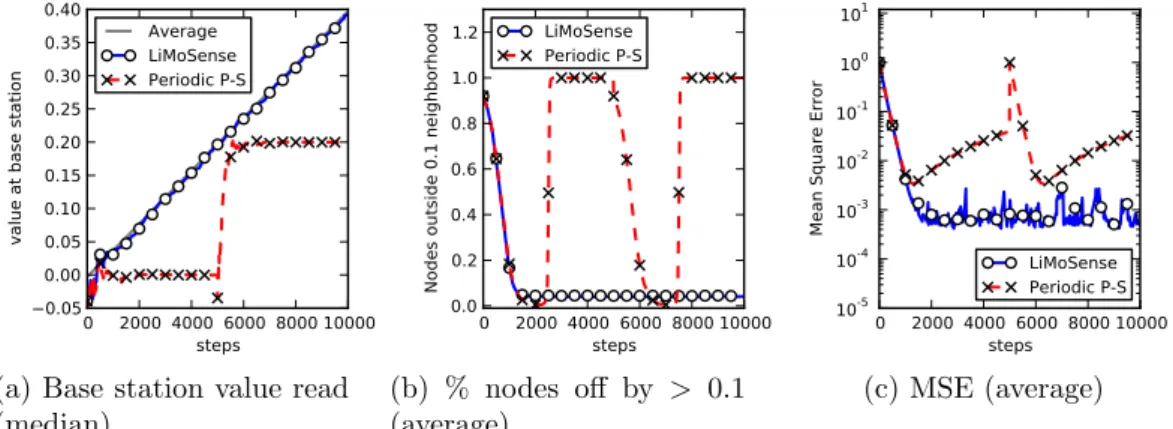
3.1 Creeping value change Every 10 steps, 5 random reads

increase by 0.01. We see that LiMoSense promptly tracks the creeping change. It provides accurate estimates to 95% of the nodes, with an MSE of about 10−3 throughout the run. The accuracy depends on the rate of change. In contrast, Periodic Push-Sum converges to the correct average only for a short period after each restart, before the average creeps away. . . . 31

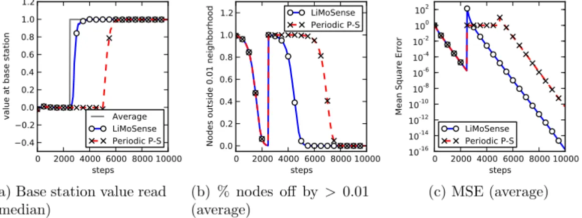
3.2 Response to a step function At step 2500, 10 random

reads increase by 10. We see that LiMoSense immediately re-acts, quickly propagating the new values. In contrast, Periodic Push-Sum starts its new convergence only after its restart. . . 32

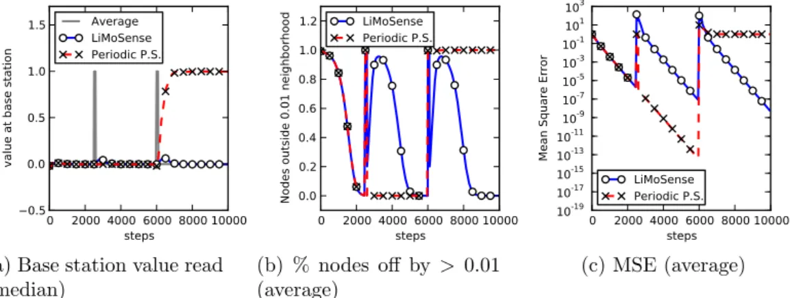
3.3 Response to impulse At steps 2500 and 6000, 10

ran-dom values increase by 10 for 100 steps. Both impulses cause temporary disturbances in the output of LiMoSense. Periodic Push-Sum is oblivious to the first impulse, since it does not react to changes. The restart of Push-Sum occurs during the second impulse, causing it to converge to the value measured then. . . 33

3.4 Failure robustness In a disc graph topology, the radio range of 10 nodes decays in step 3000, resulting in about 7 lost links in the system. Then, in step 5000, a node crashes. Each failure causes a temporary disturbance in the output of LiMoSense. Periodic Push-Sum is oblivious to the link failure. It recovers from the node failure only after the next restart. . 34

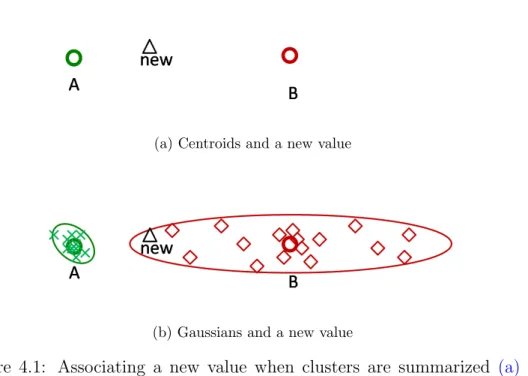
4.1 Associating a new value when clusters are summarized (a) as centroids and (b) as Gaussians. . . 50

4.2 Gaussian Mixture clustering example. The three Gaussians in Figure 4.2a were used to generate the data set in Figure 4.2b. The GM algorithm produced the estimation in Figure 4.2c. . 54

LIST OF FIGURES v

4.3 Effect of the separation of erroneous samples on the calcu-lation of the average: A 1,000 values are sampled from two Gaussian distributions (a). As the erroneous samples’ distri-bution moves away from the good one, the regular aggregation error grows linearly (b). However, once the distance is large enough, our protocol can remove the erroneous samples, which results in an accurate estimation of the mean. . . 55

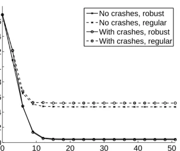
4.4 The effect of crashes on convergence speed and on the accuracy of the mean. . . 56

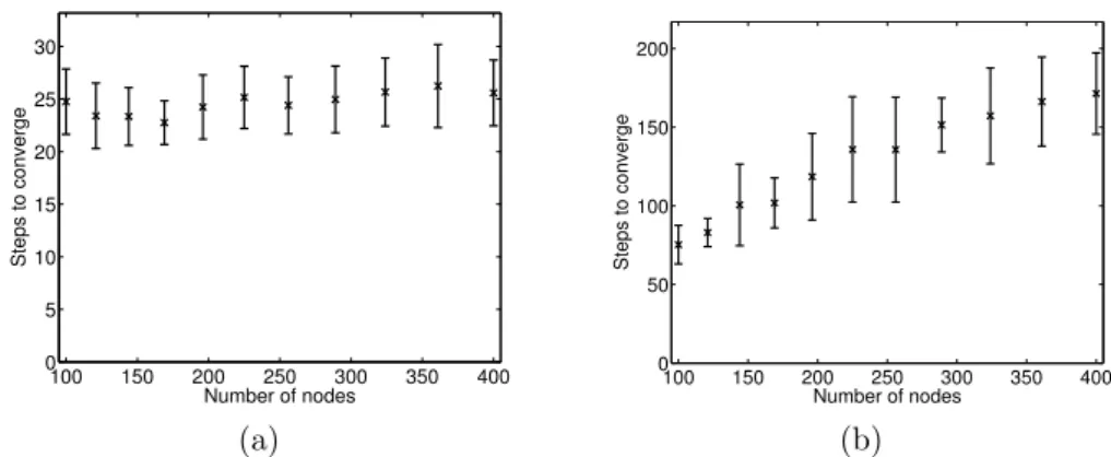
4.5 Convergence time of the distributed clustering algorithm as a function of the number of nodes (a) in a fully connected topology and (b) in a grid topology. . . 57

4.6 The angles of the vectors va and ve. . . 64

4.7 The possible constructions of two vectors va and vb and their

sum vc, s.t. their angles with the X axis are smaller than π/2

and va’s angle is larger than vb’s angle. . . 65

6.1 Simulation of the average duration of read operations shown with one concurrent writer accessing the KVS replicas at vary-ing network latencies. The mean network latency of the reader is 100 ms; only when the writer has a much smaller latency does the read operations take longer than the expected min-imum of 400 ms. . . 86

6.2 Simulation of the average duration of read operations as a function of the data size. For small values, the network latency dominates; for large value, the duration converges to the time for transferring the data. . . 87

6.3 Simulation of the average duration of write operations as a function of the number of concurrent writers. The single-writer approach with serialized operations is shown for com-parison. . . 88

6.4 Simulation of the maximal space usage depending on the num-ber of concurrent writers. The upper bound is the numnum-ber of writers plus two according to Theorem 5. . . 89

6.5 The median duration of read operations and get operations as the data size grows. The box plots also show the 30th _and the 70th _{percentile. . . . . 90} 6.6 The median duration of write operations andput operations

as the data size grows. The box plots also show the 30th _and the 70th _{percentile. . . . . 91}

LIST OF FIGURES vi

6.7 Comparison of the duration of read and writeoperations for the real system (solid lines) and the simulated system (dotted lines). The graph shows a histogram of the operation dura-tions for 1000 read operations (centered at about 1200 ms) and 1000 write operations (centered at about 1800 ms). . . . 92

7.1 Schematic structure of ACID-RAIN. Transaction Managers (TMs) 1, . . . , m access multiple objects per transaction. Ob-jects are managed (cached) by Object Managers (OMs) 1, . . . , n.

OMi(1) is falsely suspected to have failed, and therefore re-placed byOMi(2), causing them to concurrently serve the same objects. The OMs are backed by reliable logs 1, . . . , n, to which they store tentative transaction operations for serialization, as well as (later) certification results. . . 94

7.2 An example flow of the simplified algorithm. A front end runs a transaction that reads object x and writes object y. The client ends the transaction, and the TM certifies it with both relevant OMs, both going through the appropriate logs before returning their local results. The TM then sends the commit result to the client. Later, it marks the transaction in the logs (via the OMs) as committed, and then as ready to GC. . . . 101

7.3 Running with 500,000 objects, we increase the rate of incom-ing transactions, each touchincom-ing a random set of 10 objects. Increasing the number of shards (2, 4, 8, and 16) improves latency as it decreases the average queue length at the logs. . 112

7.4 For an increasing number of shards, we run multiple simu-lations to find the maximal TPUT the system can handle. We observe linear scaling for ACID-RAIN, whereas 2PC and global log reach a bound. . . 113

7.5 System behavior under a uniformly random workload. With poor prediction quality and a small number of objects the sys-tem observes high collision rates, and hence high abort rates.

. . . 115

7.6 System behavior under a hot-zone workload, where a small subset of the objects are accessed with increasing probability. With poor prediction quality we observe high collision rates, and hence high abort rates. . . 115

7.7 System behavior under a Pareto workload. With poor pre-diction quality, as the Pareto parameter increases, we observe high collision rates, and hence high abort rates. . . 116

LIST OF FIGURES vii

7.8 Commit ratio for an increasing number of objects and predic-tors with different slack values, predicting the correct access sets, twice and four times the required objects. Even with potentially high collision rates (few objects), commit ratios mostly remain high. Only for small numbers of objects, and with high slack, does the commit rate fall significantly. . . 116

7.9 Effect of an OM crash and replacement. A moving average of the normalized commit rate is shown as a function of time. The OM of one out of 5 shards crashes at time 20, and is replaced (restoring from the log) at time 70. The average commit rate (over a sliding window) drops after the crash and rises once the replacement OM is in place. . . 117

Abstract

Fast advancements in the production and construction of computer systems have led to the proliferation of highly distributed systems, at a scale that was unimaginable not many years ago. We address here two types of such systems — sensor networks and cloud storage. We construct scalable and robust distributed algorithms for these environments, prove their correctness, and analyze their behavior through simulation.

To perform monitoring of large environments, we can expect to see in years to come sensor networks with thousands of light-weight nodes mon-itoring conditions like seismic activity, humidity or temperature. Each of these nodes is comprised of a sensor, a wireless communication module to connect with close-by nodes, a processing unit and some storage. The nature of these widely-spread networks prohibits a centralized solution in which the raw monitored data is accumulated at a single location. Fortunately, often the raw data is not necessary. Rather, an aggregate that can be computed inside the network.

In the first part of this work, we address two aggregation challenges in the field of sensor networks. First, we present LiMoSense, a fault-tolerant live monitoring algorithm for dynamic sensor networks. This is the first asynchronous robust average aggregation algorithm that performs live moni-toring, i.e., it constantly obtains a timely and accurate picture of dynamically changing data. Second, we address the distributed clustering problem, where the computed aggregate is a clustering of the sensor data, i.e., the goal is to partition these values into multiple clusters, and describe each cluster con-cisely. We present a generic algorithm that solves the distributed clustering problem and may be implemented in various topologies, using different clus-tering types.

In the second part of this work, we address two challenges relating to consistency in large scale cloud storage systems. Advances in datacenter technologies are leading users, both consumers and large companies, to store large volumes of data in managed services, where storage is offered as a ser-vice — cloud storage. The users of such systems have increasing expectations

of both efficiency and reliability, leading to various challenges in implement-ing these data stores.

First, we observe that a single storage provider, large as it may be, might fail, either losing data or just being temporarily unavailable. We provide a storage algorithm that achieves reliable storage using multiple real-world production storage services. A key-value store (KVS) offers functions for storing and retrieving values associated with unique keys. KVSs have be-come the most popular way to access Internet-scale “cloud” storage sys-tems. We present an efficient wait-free algorithm that emulates multi-reader multi-writer storage from a set of potentially faulty KVS replicas in an asyn-chronous environment.

Second, we introduce ACID-RAIN: ACID1 _{transactions in a Resilient}

Archive with Independent Nodes. ACID-RAIN is a novel architecture for ef-ficiently implementing transactions in a distributed data store. ACID-RAIN uses logs in a novel way, limiting reliability to a single tier of the system: a large and scalable set of independent nodes form an outer layer that caches the data, backed by a set of independent reliable log services. If concur-rent transactions conflict with one another, one or more of them must abort. ACID-RAIN avoids such conflicts by using prediction to order transactions before they take actions that would lead to an abort.

1_{“ACID transactions”, stands for Atomic, Consistent, Isolated and Durable}

transac-tions. These are commonly known in the distributed systems literature as atomic trans-actions with persistent storage.

Chapter 1

Introduction

The field of distributed computing has been dealing for a long while with challenges of designing robust and scalable algorithms for different purposes, from data acquisition, through processing, to storage. Recently, advance-ments in the production and construction of large scale networked systems has made such algorithms a practical necessity. The design of a distributed algorithm has to follow the following principles.

Robustness A system with thousands of nodes naturally suffers from occa-sional node failures, and consequently new node additions. Similarly, message loss and link failure are unavoidable in large systems, and the system must be resilient to all of these.

Asynchrony Synchronous algorithms make assumptions on the maximal delay in the system. This allows a node to deduce, by waiting this de-lay, that a message it has sent was received, or that if it does not receive a message, that message was never sent, or was lost. Using a conserva-tive assumption (large delay) causes the system to progress slowly, as nodes have to wait long to make these deduction. However, choosing a shorter delay is not an option — in a large system occasional occur-rences of long delays are the norm. A single node may suffer from a temporal malfunction slowing it down considerably, and messages may be delayed in a multi-hop network. A system should therefore avoid these assumptions, and use an asynchronous algorithm that makes no assumptions on message delay.

Scalability To be truly scalable, a system must refrain from depending on any single element in its critical path, since this element will become a bottleneck.

This dissertation describes four scalable algorithms that follow these prin-ciples. They are all asynchronous, allow for node and link failure, and depend on no single element for operation.

1.0.0..1 Aggregation in sensor networks In Part I we address two aggregation challenges in the field of sensor networks. Sensor networks are ad-hoc networks of light-weight nodes monitoring environmental conditions, each communicating via radio with close-by nodes. We briefly introduce aggregation in sensor networks in Chapter 2.

In Chapter3, we present LiMoSense, a fault-tolerant live monitoring al-gorithm for dynamic sensor networks. This is the first asynchronous robust average aggregation algorithm that performs live monitoring, i.e., it con-stantly obtains a timely and accurate average of dynamically changing data. However, more elaborate data summaries are sometimes required. For example, outliers caused by erroneous samples may divert the average, or the data may be partitioned into several clusters with different averages. In Chapter4we address the distributed clustering problem, where the computed aggregate is a clustering of the sensor data, i.e., the goal is to partition the values into multiple clusters, and describe each cluster concisely. We present a generic algorithm that solves the distributed clustering problem and may be implemented in various topologies, using different clustering types. As an example, we implement Gaussian mixture clustering and evaluate its accuracy and convergence speed through simulation.

1.0.0..2 Consistency in Cloud Storage In PartII, we present two al-gorithms that deal with distributed cloud storage. Cloud storage allows many users to concurrently access replicated data stored on multiple machines re-siding in datacenters. We provide the relevant background in Chapter 5.

Cloud storage providers typically offer several storage interfaces, each implementing different interfaces. However, practically all providers offer a key-value store (KVS), with functions for storing and retrieving values asso-ciated with unique keys. Cloud storage providers promise high availability, but even the largest of them sometimes fail, either losing data or just being temporarily unavailable.

In Chapter6we present a storage algorithm that provides reliable storage using multiple real-world production storage services. We present an efficient wait-free algorithm that provides multi-reader multi-writer storage from a set of potentially faulty KVS replicas in an asynchronous environment.

In cloud-scale data centers, it is common to shard data across many nodes, each maintaining a small subset of the data. Although ACID transactions are

desirable, architects of such systems often tradeoff efficiency for consistency, and do not support them. In Chapter 7 we present a novel architecture for support of low-latency high-throughput ACID transactions in a Resilient Archive with Independent Nodes (ACID-RAIN). ACID-RAIN uses logs in a novel way, limiting the requirement for reliability to a single scalable tier: A set of independent highly-available logs is accessed by large set of independent fault-prone nodes that caches the sharded data. This structure allows for rapid data access through the cache, and simple and fast restoration in case of node failure. ACID-RAIN dramatically reduces concurrency conflicts by using prediction to order transactions before they take actions that would lead to an abort. We compare ACID-RAIN with contemporary architectures for the support of ACID transactions, and demonstrate effective contention handling and linear scalability, whereas other approaches reach a bottleneck.

Part I

Aggregation in Sensor

Networks

Chapter 2

Background

To perform monitoring of large environments, we can expect to see in years to come sensor networks with thousands of light-weight nodes monitoring conditions like seismic activity, humidity or temperature [10, 105]. Each of these nodes is comprised of a sensor, a wireless communication module to connect with close-by nodes, a processing unit and some storage. The nature of these widely spread networks prohibits a centralized approach in which the raw monitored data is accumulated at a single location. Specifically, all sensors cannot directly communicate with a central unit.

Fortunately, often the raw data itself is not the goal. Rather, anaggregate

that can be computedinside the network, such as the sum or average of sensor reads, is of interest. For example, when measuring rainfall, one is interested only in the total amount of rain, and not in the individual reads at each of the sensors. Similarly, one may be interested in the average humidity or temperature rather than minor local irregularities.

Several works have dealt with the single-shot version of this problem [72,

21, 87, 83]. In the single-shot case, each sensor takes a single sample, and then the nodes communicate and learn the average of these read-values. How-ever, to perform live monitoring, we need to constantly obtain a timely and accurate picture of the ever-changing data. Running multiple iterations of a single-shot algorithm is either inefficient (starting iterations with high fre-quency) or inaccurate (starting them with a low frequency, or not allowing the runs to converge). In Chapter 3we tackle the problem of live monitoring in a dynamic sensor network. This problem is particularly challenging due to the dynamic nature of sensor networks, where nodes may fail and may be added on the fly (churn), and the network topology may change due to battery decay or weather change.

While average aggregation is useful in many scenarios, there are applica-tions that call for a more elaborate summarization of the sensors’ readings. In

the distributed clustering problem, numerous interconnected nodes compute a clustering of their data, i.e., partition these values into multiple clusters, and describe each cluster concisely.

We present in Chapter 4 a generic algorithm that solves the distributed clustering problem and may be used in any connected topology, using differ-ent clustering types. For example, the generic algorithm can be instantiated to cluster values according to distance, targeting the same problem as the famous k-means clustering algorithm. Since the distance criterion is often not sufficient to provide good clustering results, we present an instantiation of the generic algorithm that describes the values as a Gaussian Mixture (a set of weighted normal distributions), and uses machine learning tools for clustering decisions. Simulations show the robustness, speed and scalability of this algorithm. We prove that any implementation of the generic algo-rithm converges over any connected topology, clustering criterion and cluster representation, in fully asynchronous settings.

Chapter 3

LiMoSense

The subject of environmental monitoring is gaining increasing interest in recent years. Live monitoring is necessary for research, and it is critical for protecting the environment by quickly discovering fire outbreaks in distant areas, cutting off electricity in the event of an earthquake, etc. In order to perform these tasks, it is necessary to perform constant measurements in wide areas, and collect this data quickly.

However, most previous solutions have focused on a static (single-shot) version of the problem, where the average of a single input-set is calcu-lated [72, 21, 87, 83]. Though it is in principle possible to perform live monitoring using multiple iterations of such algorithms, this approach is not adequate, due to the inherent tradeoff it induces between accuracy and speed of detection. For further details on previous work, see Section 3.1. In this chapter we tackle the problem of live monitoring in a dynamic sensor network. This problem is particularly challenging due to the dynamic nature of sensor networks, where nodes may fail and may be added on the fly (churn), and the network topology may change due to battery decay or weather change. The formal model and problem definition appear in Section 3.2.

In Section 3.3 we present our new LiveMonitoring for Sensor networks algorithm, LiMoSense. Our algorithm computes the average over a dynami-cally changing collection of sensor reads. The algorithm has each node calcu-late an estimate of the average, which continuously converges to the current average. The space complexity at each node is linear in the number of its neighbors, and message complexity is that of the sensed values plus a con-stant. At its core, LiMoSense employs gossip-based aggregation [72,87], with a new approach to accommodate data changes while the aggregation is on-going. This is tricky, because when a sensor read value changes, its old value should be removed from the system after it has propagated to other nodes. LiMoSense further employs a new technique to accommodate message loss,

failures, and dynamic network behavior in asynchronous settings. This is again difficult, since a node cannot know whether a previous message it had sent over a faulty link has arrived or not.

In Section 3.4, we prove the correctness of the algorithm, showing that once the network stabilizes, in the sense that no more value or topology changes occur, LiMoSense eventually converges to the correct average, de-spite message loss. Since the algorithm cannot tell if and when the network has stabilized, it constantly converges to the current average.

To demonstrate the effectiveness of LiMoSense in various dynamic sce-narios, we present in Section3.5 results of extensive simulations, showing its quick reaction to dynamic data read changes and fault tolerance. In order to preserve energy, communication rates may be decreased, and nodes may switch to sleep mode for limited periods. These issues are outside the scope of this work.

In summary, this chapter makes the following contributions:

1. It presents LiMoSense, a live monitoring algorithm for highly dynamic and error-prone environments.

2. It proves correctness of the algorithm, namely robustness and eventual convergence.

3. It shows by simulation that LiMoSense converges exponentially fast in well connected topologies, and demonstrates its efficiency and fault-tolerance in dynamic scenarios.

A preliminary version of the work presented in this chapter appears in the proceedings of the 7th International Symposium on Algorithms for Sen-sor Systems, Wireless Ad Hoc Networks and Autonomous Mobile Entities (ALGOSENSOR’11) [48].

3.1

Related Work

To gather information in a sensor network, one typically relies on in-network

aggregation of sensor reads. The vast majority of the literature on ag-gregation has focused on obtaining a single summary of sensed data, as-suming these reads do not change while the aggregation protocol is run-ning [83, 72, 21, 87].

For obtaining a single aggregate, two main approaches were employed. The first is hierarchical gathering to a single base station [83]. The hierar-chical method incurs considerable resource waste for tree maintenance, and results in aggregation errors in dynamic environments, as shown in [64].

The second approach is gossip-based aggregation at all nodes. To avoid counting the same data multiple times, Nath et al. [88] employ order and duplicate insensitive (ODI) functions to aggregate inputs in the face of mes-sage loss and a dynamic topology. However, these functions do not support dynamic inputs or node failures. Moreover, due to the nature of the ODI functions used, the algorithms’ accuracy is inherently limited – they do not converge to an accurate value [50].

An alternative approach to gossip-based aggregation is presented by Kempe et al. [72]. They introduce Push-Sum, an average aggregation algorithm, and bound its convergence rate, showing that it converges exponentially fast in fully connected networks where nodes operate in lock-step. Fangani and Zampieri [49] analyze the exact convergence rate for a fully connected net-work, and Boyd et al. [22] analyze this algorithm in an arbitrary topology. Jelasity et al. [67] periodically restart the push-sum algorithm to handle dynamic settings, trading off accuracy and bandwidth. Although these algo-rithms do not deal with dynamic inputs and topology as we do, we borrow some techniques from them. In particular, our algorithm is inspired by the Push-Sum construct, and operates in a similar manner in static settings. The aforementioned analyses therefore apply to our algorithm if and when the system stabilizes.

We are aware of two approaches to aggregate dynamic inputs. The first, by Birk et al. [18], is limited to unrealistic settings, namely a static topology with reliable communication links, failure freedom, and synchronous oper-ation. The second approach, called flow updates [69, 68, 5] also solves ag-gregation in dynamic settings, overcoming message loss, dynamic topology and churn, albeit in synchronous settings only, running in rounds. Though the technique is illustrated to work in one simulation with dynamic inputs, the correctness proof and analysis [5] cover static inputs only, and the paper does not prove converge to the correct average in the face of message loss. Fi-nally, Flow-Update requires maintaining the aggregate of the messages sent on a link, resulting in an unbounded variable size, a challenge LiMoSense overcomes.

Note that aggregation in sensor networks is distinct from other aggre-gation problems, such as stream aggreaggre-gation, where the data in a sliding window is summarized. In the latter, a single system component has the entire data, and the distributed aspects do not exist.

3.2

Model and Problem Definition

3.2.1

Model

The system is comprised of a dynamic set of nodes (sensors), partially con-nected by dynamic undirected communication links. Two nodes concon-nected by a link are called neighbors, and they can send messages to each other. These messages either arrive at some later time, or are lost. Messages that are not lost on each link arrive in FIFO order. Links do not generate or duplicate messages.

The system is asynchronous and progresses in steps, where in each step an event happens and the appropriate node is notified, or a node acts spon-taneously. Spontaneous steps occur infinitely often. In a step, a node may change its internal state and send messages to its neighbors.

Nodes can be dynamically added to the system, and may fail or be re-moved from the system (churn). The set of nodes at timetis denotedNt_and

their number nt. The system state at time t consists of the internal states of all nodes in Nt_{, and the links among them. When a node is added (init}

event), it is notified, and its internal state becomes a part of the system state. When it is removed (remove event), it is not allowed to perform any action, and its internal state is removed from the system state.

Each sensor has a time varyingdata read in_R. A node’s initial data read is provided as a parameter when it is notified of its init event. This value may later change (changeevent) and the node is notified with the newly read value. For a node i in Nt_{, we denote}1 _{by r}t

i, the latest data read provided

by an init orchange event at that node before timet.

Communication links may be added or removed from the system. A node is notified of link addition (addNeighborevent) and removal (removeNeighbor event), given the identity of the link that was added or removed. We call these topology events2_{. For convenience of presentation, we assume that}

ini-tially, nodes have no links, and they are notified of their neighbors by a series of addNeighbor events. We say that a link (i, j) is up at step t if by step

t, both nodesi and j had received an appropriate addNeighbornotification and no later removeNeighbor notification. Note that a link (i, j) may be

half-up in the sense that the node i was notified of its addition but node j

was not, or if node j had failed.

A node may send messages on a link only if the last message it had

1_{For any variable, the node it belongs to is written in subscript and, when relevant,}

the time is written in superscript.

2_{There is a rich literature dealing with the means of detecting failures, usually with}

received regarding the state of the link is addNeighbor. If this is the case, the node may also receive a message on the link (receiveevent).

3.2.1..3 Global Stabilization Time We defineglobal stabilization time, GST, to be the first time from which onward the following properties hold: (1) The system isstatic, i.e., there are nochange,init,remove,addNeighbor orremoveNeighbor events. (2) If the latest topology event a nodei∈ NGST

has received for another node j is addNeighbor, then node j is alive, and the latest topology event j has received for iis alsoaddNeighbor(i.e., there are no half-up links). (3) The network is connected. (4) If a link is up after GST, and infinitely many messages are sent on it, then infinitely many of them arrive.

3.2.2

The Live Average Monitoring Problem

We define theread averageof the system at timetasRt=∆ _|N1t_| P

i∈Ntrt_i.Note

that the read average does not change after GST. Our goal is to have all nodes estimate the read average after GST. More formally, an algorithm solves the

Live Average Monitoring Problem if it gets time-varying data reads as its inputs, and has nodes continuously output their estimates of the average, such that at every node in NGST_{, the output estimate converges to the read}

average after GST.

3.2.2..4 Metrics We evaluate live average monitoring algorithms using the following metrics: (1)Mean square error,MSE, which is the mean of the squares of the distances between the node estimates and the read average; and (2) ε-inaccuracy, which is the percentage of nodes whose estimate is off by more than ε.

3.3

The LiMoSense Algorithm

In Section 3.3.1 we describe a simplified version of the algorithm for dy-namic inputs but static topology and no failures. This simplified version demonstrates our novel approach for handling dynamic inputs. However, this simplified version is unable to accommodate topology changes, churn, and message loss. To overcome these, we present in Section 3.3.2 a robust algorithm, in which each node maintains for each of its links a summary of the data communicated over that link thereby enabling it to recover after these changes. These summaries, however, are aggregates of all exchanges on the links, and their size grows unboundedly. In Section3.3.3, we describe

Algorithm 1: Failure-Free Dynamic Algorithm 1 state 2 (est_i, w_i)∈_R2 3 prevReadi∈R 4 oniniti(initVal) 5 (est_i, w_i)←(initVal,1) 6 prevReadi←initVal 7 onreceivei((vin, win)) fromj 8 (est_i, w_i)←(est_i, w_i)⊕(vin, win) 9 periodicallysendi()

10 Choose a neighborjuniformly at random. 11 w_i←w_i/2 12 send ((est_i, w_i)) toj 13 onchange_i(newRead) 14 est_i←est_i+_w1 i ·(newRead−prevReadi) 15 prevReadi←newRead

the complete LiMoSense algorithm, which also implements a clearing mech-anism that results in bounded sizes of all its variables and messages, without resorting to atomicity or synchrony assumptions.

3.3.1

Failure-Free Dynamic Algorithm

We begin by describing a version of the algorithm that handles dynamically changing inputs, but assumes no message loss or link or node failures. The pseudocode is shown in Algorithm 1.

The base of the algorithm operates like Push-Sum [72, 21]: Each node maintains a weighted estimate of the read average (a pair containing the esti-mate and a weight), which is updated as a result of the node’s communication with its neighbors. As the algorithm progresses, the estimate converges to the read average.

In order to accommodate dynamic reads, a node whose read value changes must notify the other nodes. It not only needs to introduce the new value, but also needs to undo the effect of its previous read value, which by now has partially propagated through the network.

The algorithm often requires nodes to merge two weighted values into one. They do so using the weighted value sum operation, which we define below and concisely denote by ⊕. Subtraction operations will be used later, they are denoted by and are also defined below. The ⊕ and operations are undefined when the sum (resp. difference) between the weights of the operands is zero. We note that the ⊕ operation is commutative and both

operations are associative. (va, wa)⊕(vb, wb) ∆ = (vawa+vbwb wa+wb , wa+wb) . (3.1) (va, wa) (vb, wb) ∆ = (va, wa)⊕(vb,−wb). (3.2)

The state of a node (lines 2–3) consists of a weighted value, (est_i, w_i), where est_i is an output variable holding the node’s estimate of the read average, and the value prevRead_i of the latest data read. We assume at this stage that each node knows its set of neighbors. We shall remove this assumption later, in the robust LiMoSense algorithm.

Node iinitializes its state on its init event. The data read is initialized to the given value initVal, and the estimate is (initVal,1) (lines 5–6).

The algorithm is implemented with the functions receive and change, which are called in response to events, and the functionsend, which is called periodically.

Periodically, a node i shares its estimate with a neighbor j chosen uni-formly at random (line 10). It transfers half of its estimate to node j by halving the weight w_i of its locally stored estimate and sending the same weighted value to that neighbor (lines 11-12). When the neighbor receives the message, it merges the accepted weighted value with its own (line 8). Nodes keep their weights larger than some small arbitrary size q, by per-forming asendonly if the node’s weight is larger than 2q. A small value ofq

therefore increases the weight sending frequency among nodes, but it does not affect the accuracy of estimation.

Correctness of the algorithm in static settings follows from two key obser-vations. First, safety of the algorithm is preserved, because the system-wide weighted average over all weighted-value estimate pairs at all nodes and all communication links is always the correct read average; this invariant is pre-served by send and receive operations. Thus, no information is ever “lost”. Second, the algorithm’s convergence follows from the fact that when a node merges its estimate with that received from a neighbor, the result is closer to the read average.

We proceed to discuss the dynamic operation of the algorithm. When a node’s data read changes, the read average changes, and so the estimate should change as well. Let us denote the previous read of node i by r_it−1

and the new read at step t by rt

i. In essence, the new read, rti, should be

added to the system-wide estimate with weight 1, while the old read, r_it−1, ought to be deducted from it, also with weight 1. But since the old value has been distributed to an unknown set of nodes, we cannot simply “recall” it. Instead, we make the appropriate adjustment locally, allowing the natural flow of the algorithm to propagate it.

We now explain how we compute the local adjustment. The system-wide estimate should shift by the difference between the read values, factored by the relative influence of a single sensor, i.e., 1/n. So an increase of x

increases the system-wide estimate by x/n. However, when a node’s read value changes, its estimate has an arbitrary weight ofw, so we need to factor the change of its value by 1/w to obtain the required system-wide shift. Therefore, in response to a change event at time t, if the node’s estimate before the change was estt_i−1 and its weight was wt_i−1, then the estimate is updated to (lines 14-15)

estt_i =estt_i−1 + (r_it−rt_i−1)/w_it−1 .

Note that the value of nt _{does not appear in the equation, as it is unknown}

to any of the nodes.

3.3.2

Adding Robustness

Overcoming failures is challenging in an asynchronous system, where a node cannot determine whether a message it had sent was successfully received. In order to overcome message loss and link and node failure, each node main-tains a summary of its conversations with each of its neighbors. Each node i

maintains the aggregates (as weighted sums) of the messages received from and sent to nodej in the variablesreceivedTotal_i(j) andsentTotal_i(j), respec-tively. Nodes interact by sending and receiving these summaries, rather than weighted values as in the failure-free algorithm. The data in each message subsumes all previous value exchanges on the same link. Thus, if a message is lost, the lost data is recovered once an ensuing message arrives. When a link fails, the nodes at both of its ends use the summaries to retroactively cancel the effect of all the messages ever transferred over it. A node failure is treated as the failure of all its links. The resulting algorithm, whose pseu-docode is given in Algorithm 2, is robust to message loss, link failure, and churn.

To send, node i adds to sentTotal_i(j) the weighted value it wants to send, and sends sentTotal_i(j) to j (lines 18–20). When receiving this mes-sage, node j calculates the newly received weighted value by subtracting its

receivedTotal_i(j) variable from the newly received aggregate (line 22). After acting on the received message (line 23), node j replaces its receivedTotal

variable with the new weighted value (line 24). Thus, if a message is lost, the next received message compensates for the loss and brings the receiving neighbor to the same state it would have reached had it received the lost messages as well. Whenever the most recent message on a link (i, j) is cor-rectly received and there are no messages in transit, the value of sentTotalj_i

Algorithm 2: Robust Dynamic Algorithm with Unbounded State

1 state

2 (est_i, w_i)∈_R2

3 prevReadi∈R

4 neighborsi⊂N,initially∅

5 sentTotal_i:N→R2,initially∀j:sentTotali(j) = (0,0)

6 receivedTotali:N→R2,initially∀j:receivedTotali(j) = (0,0)

7 (unrecvVali,unrecvWeighti)∈R2,initially(0,0)

8 oniniti(initVal)

9 (esti, wi)←(initVal,1)

10 prevReadi←initVal

11 periodicallysendi()

12 Choose a neighborjuniformly at random. 13 ifw_i>= 2q then

14 wtoUnsend←max(unrecvWeighti, wi−q)

15 (est_i, w_i)←(est_i, w_i) (unrecvVal_i, wtoUnsend)

16 unrecvWeighti←unrecvWeighti−wtoUnsend

17 ifw_i>= 2qthen

18 sentTotal_i(j)←sentTotal_i(j)⊕(est_i, w_i/2) 19 (est_i, w_i)←(est_i, w_i/2)

20 sendsentTotal_i(j) toj

21 onreceivei(vin, win) fromj

22 diff←(vin, win) receivedTotali(j)

23 (est_i, w_i)←(est_i, w_i)⊕diff 24 receivedTotali(j)←(vin, win)

25 onchangei(rnew)

26 esti←esti+w1_i ·(rnew−prevReadi)

27 prevReadi←rnew

28 onaddNeighbor_i(j)

29 neighborsi←neighborsi∪ {j}

30 onremoveNeighbori(j)

31 (est_i, w_i)←(est_i, w_i)⊕sentTotali(j)

32 (unrecvVal,unrecvWeight)←(unrecvVal,unrecvWeight)⊕receivedTotal_i(j) 33 neighborsi←neighborsi\ {j}

34 sentTotal_i(j)←(0,0) 35 receivedTotali(j)←(0,0)

is identical to the value of receivedTotali_j. In order to overcome message loss, a node i sends its summary to its neighbor j even if its current weight is smaller than 2q, and the message carries no new information.

Upon notification of topology events, nodes act as follows. When noti-fied of an addNeighbor event, a node simply adds the new neighbor to its

neighbors list (line 29). When notified of a removeNeighbor event, a node reacts by nullifying the effect of this link, clearing the state variables, re-moving the neighbor from its neighbors list, and discarding its link records (lines 31–35). The effects of sent and received messages are summarized in the respectivesentTotal andreceivedTotalvariables. When a nodeidiscovers that link (i, j) failed, it adds the outgoing link summarysentTotalj_i to its es-timate, thus cancelling the effect of ever having sent anything on the link. In

order to prevent its estimate weight from becoming negative, receivedTotalj_i

is not immediately subtracted from the estimate. Instead, the node adds the incoming link summary receivedTotalj_i to a buffer, the weighted value (unrecvVal,unrecvWeight) and lazily subtracts it from its estimate, preserv-ing the estimate weight positive (lines 13–16). The node thus cancels the effect of everything it has received from that neighbor.

After a node joins the system or leaves it, its neighbors are notified of the appropriate topology events, adding links to the new node, or removing links to the failed one. Thus, when a node fails, any part of its read value that had propagated through the system is annulled, and it no longer contributes to the system-wide estimate.

3.3.3

LiMoSense

The summary approach of Algorithm 2 causes summary sizes, namely the weights of receivedTotal_i(j) and sentTotal_i(j), to increase unboundedly as the algorithm progresses. To avoid that, we devise a channel reset mecha-nism that prevents this without resorting to synchronization assumptions. Instead of storing the aggregates of all received and sent weights, we store only their difference, which can be bounded, and we store the received and sent aggregates only for limited epochs, thereby bounding them as well.

The result is the full LiMoSense algorithm, shown as Algorithms 3–4, where the state information of Algorithm2is replaced with a more elaborate scheme. Messages are aggregated in epochs, and the aggregate is reset on epoch change. Epochs are defined per node, per link, and per direction, and are identified by binary serial numbers, so each node maintains an incoming and an outgoing serial number per link. Node i maintains for its link with nodejthe serial numbersinSN_i(j) andoutSN_i(j) for the incoming and outgo-ing weights, respectively. Epochs on different directed links are independent of each other. Neighboring nodes reset their aggregates for their connect-ing directed link and proceed to the next epoch after reachconnect-ing consensus on the aggregate values sent in the current epoch. This approach is similar to the classical stop-and-wait message exchange protocol [100]. However, here the receiving end of the link initiates the transition to the next epoch, after receiving multiple messages. Intuitively, the stop-and-wait is performed for the ACKs, each of which acknowledges a set of weight transfers.

For a link (i, j), nodeimaintains insent_i(j) andreceived_i(j) the aggregate sent and received values in the current epoch (rather than the entire history as in the failure-free algorithm). In addition, it maintains intotalDiff_i(j) the difference between the sent and received aggregates over the entire history.

Algorithm 3: LiMoSense – part 1

1 state

2 (est_i, w_i)∈_R2

3 prevReadi∈R

4 neighborsi⊂N,initially∅

5 totalDiff_i:N→R2,initially∀j:totalDiffi(j) = (0,0)

6 (unrecvVali,unrecvWeighti)∈R2,initially(0,0)

7 sent_i:N→R2,initially∀j:sent_i(j) = (0,0)

8 outSN_i:N→ {0,1},initially∀j:outSNi(j) = (0,0) (Serial number of outgoing messages)

9 receivedi:N→R2,initially∀j:receivedi(j) = (0,0)

10 inSN_i:N→ {0,1},initially∀j:inSNi(j) = 0 (Expected serial number of incoming messages)

11 clearedi:N→R2,initially∀j:clearedi(j) = (0,0) (Weight received with previous serial number)

12 oniniti(initVal)

13 (est_i, w_i)←(initVal,1) 14 prevReadi←initVal

15 periodicallysendi()

16 Choose a neighborjuniformly at random. 17 ifw_i>= 2q then

18 wtoUnsend←max(unrecvWeighti, wi−q)

19 (est_i, w_i)←(est_i, w_i) (unrecvVal_i, wtoUnsend)

20 unrecvWeight_i←unrecvWeight_i−wtoUnsend

21 ifw_i>= 2qandweight of totalDiffi(j)>−2·boundandweight of senti(j)<2·bound then

22 sent_i(j)←sent_i(j)⊕(est_i, w_i/2) (sentTotal_i(j)←sentTotal_i(j) + (est_i, w_i/2)) 23 totalDiff_i(j)←totalDiff_i(j) (est_i, w_i/2)

24 (est_i, w_i)←(est_i, w_i/2)

25 send (sent_i(j),outSN_i(j),inSN_i(j)−1 mod 2,cleared_i(j)) toj (Ack cleared vals and serial of previous epoch)

26 onreceivei((vin, win),msgSN,clearSN,clearVal) fromj

27 ifclearSN=outSNi(j)then (Relevant clear)

28 outSNi(j)←outSNi(j) + 1 mod 2

29 sent_i(j)←sent_i(j) clearVal (sentClearedi(j)←sentClearedi(j) +clearVal)

30 ifmsgSN=inSNi(j)then (Relevant message)

31 diff←(vin, win) receivedi(j)

32 (est_i, w_i)←(est_i, w_i)⊕diff 33 totalDiff_i(j)←totalDiff_i(j)⊕diff

34 receivedi(j)←(vin, win) (receivedTotali(j)←receivedTotali(j) +diff)

35 if (weight of receivedi(j))>bound then (Reset the channel)

36 inSN_i(j)←inSN_i(j) + 1 mod 2 37 cleared_i(j)←received_i(j)

(receivedCleared_i(j)←receivedCleared_i(j) +received_i(j)) 38 receivedi(j)←(0,0)

that the weight in received_i(j) reaches a certain threshold (line 35). Node j

then (1) increments modulo 2 the serial number on that link, (2) adds the aggregate received values in the completed epoch to itstotalDiff_i(j) summary of the link, and (3) clears the aggregate by storing received_i(j) in cleared_i(j) and setting received_i(j) to zero (lines 36–38). Node j will not accept future messages for the previous serial number — it will simply ignore them. On its next send toi(in the inverse direction), nodej’s message will updateiabout

Algorithm 4: LiMoSense – part 2

39 onchangei(rnew)

40 esti←esti+w1_i ·(rnew−prevReadi)

41 prevReadi←rnew 42 onaddNeighbor_i(j) 43 neighborsi←neighborsi∪ {j} 44 inSNi(j)←0 45 outSNi(j)←0 46 onremoveNeighbori(j)

47 ifWeight of totalDiffi(j)<0 then

48 (est_i, w_i)←(est_i, w_i) totalDiff_i(j)

49 else

50 (unrecvVal_i,unrecvWeight_i)←(unrecvVal_i,unrecvWeight_i)⊕totalDiff_i(j) 51 neighborsi←neighborsi\ {j}

52 totalDiffi(j)←(0,0) (receivedClearedi(j)←(0,0),sentClearedi(j)←(0,0))

53 sent_i(j)←(0,0) 54 received_i(j)←(0,0) 55 cleared_i(j)←(0,0)

the epoch reset by sending the index and final aggregate of the completed epoch (line 25).

When notified of the channel reset, the sender resets the aggregate for that channel, and increases modulo 2 the serial number as well. Note that i

may have sent messages with the old serial number after the receiver reset the link, but these messages are ignored by j. To prevent this weight from being lost, node i does not reset its aggregate to zero, but rather to the aggregate of messages sent with the old serial number but not cleared (line 29).

Upon notification of topology events, nodes act as follows. When notified of an addNeighborevent, a node adds the new neighbor to itsneighbors list and resets the epoch serial numbers for the link (lines43–45). When notified of a removeNeighborevent, a node removes the neighbor from its neighbors

list and discards its link records. Additionally, it subtracts totalDiff from its estimate, thus cancelling the effect of ever having communicated over the link. Unlike Algorithm2, we cannot separate here the sent from the received weights. To prevent the estimate weight from being negative, we check if the weight in totalDiff is positive. If it is, we add to an aggregate buffer (unrecvVal,unrecvWeight), which is later subtracted in stages fromtotalDiff

(on send events), as before.

We follow in comments the behavior of four virtual variables, the to-tal sent and received aggregates in sentTotal_i(j) and receivedTotal_i(j), re-spectively, and the aggregates of everything that was ever cleared from

sent_i(j) and received_i(j) in sentCleared_i(j) and receivedCleared_i(j), respec-tively. These virtual variables all grow unboundedly as the algorithm pro-gresses and we will use them for proving correctness in Section 3.4.

3.4

Correctness

In this section, we show that the LiMoSense algorithm (Algorithms 3–4) adapts to network topology as well as value changes and converges to the correct average. We start in Section3.4.1 by proving that when there are no half-up links, a combination of the system’s variables equals the read sum. Then, in Section 3.4.2, we prove that after GST the estimates at all nodes eventually converge to the average of the latest read values.

3.4.1

Invariant

We denote by (Rt, nt) the read sum at timet, as shown in Equation3.3. (Rt, nt) =

n

M

i=1

(rt_i,1) (3.3)

We denote by (Et, n) the weighted sum over all nodes at time t of their (1) weighted values, (2) outgoing link summaries in their sent variables, (3) the inverse of their incoming summaries in their received variables, and (4) the latestcleared received aggregate, if their neighbor has not yet received the reset message. The sum is shown in Equation 3.4

(Et, nt) = n M i=1      

(estt_i, wt_i) (unrecvValt_i,unrecvWeightt_i)⊕

⊕ M j∈neighborsti sentt_i(j) receivedt_i(j) M j∈neighborst_is.t. inSNt_i(j)6= outSNt_j(i) clearedt_i(j)       (3.4)

We show that if there are no half-up links in the system (each link is known to be up or down by both its nodes), then Rt =Et.

Lemma 1. For any timet, if for any nodes iandj, eitherj ∈neighborst_i∧i∈

neighborst_j or j 6∈neighborst_i∧i6∈neighborst_j, then Rt_=Et_.

We begin by analyzing the effect of communication steps, then of dynamic steps, and then conclude by proving the statement.

Static Behavior

First, we consider send and receive events. Note that message loss is not an event and does not affect the state of the system. In particular, it does not affect the correctness of this lemma or the following ones.

Lemma 2 (Static operations). If step t is either send or receive at some node i, then Rt_−Et_=Rt−1_−Et−1 _.

Proof. First, consider a send step. If the weight in i is below the threshold of 2q, no variables are changed (lines17and21), so the lemma trivially holds. If the weight is above the threshold, then a certain weight is subtracted from the pairs (unrecvValt_i−1,unrecvWeightt_i−1) and (est_it−1, wt_i−1) (lines 18– 20). Since the two pairs appear with opposite signs in Equation 3.4, the value of

E is unchanged. If the weight in i is still above the threshold of 2q, then the weighted value (estt_i−1,1₂w_it−1) is subtracted from the weighted value of node i, and added to sentj_i, again leaving (Et_{, n) according to Equation 3.4}

unchanged.

Next consider a receive step. Lines 27–29 handle the outgoing link to

j. If the message’s clearSN is the same as the current outSN_i(j) (line 27), it causes a reset. Node i reacts by resetting sent_i(j) and incrementing

outSN_i(j). IncrementingoutSN_i(j) makes it equal to its counterpartinSN_j(i), removing the negativecleared_j(i) element from the sum in Equation3.4. De-creasing sent_i(j) by the same value, leaves Et in Equation 3.4 unchanged.

Next, if the incoming message carries the appropriate serial number, the incoming value (deducting the previously received value from the incoming aggregate) is added to the weighted value of node j, and the same weighted value is added to receivedi_j. Since the latter is subtracted in Equation 3.4, this leaves (Et_{, n) unchanged.}

Finally, if the weight in the incoming message is too high, the receiver ini-tiates a channel reset. Note that the incoming message serial number equals

outSN_j(i). The node increments inSN_i(j), causing cleared_i(j) to be counted in the sum, since after the change it becomes different thanoutSN_j(i). Then it stores the value ofreceived_i(j) incleared_i(j), and nullifiesreceived_i(j), both with negative sign in Equation 3.4, leaving (Et_{, n) unchanged.}

None of these events changes the read sum, therefore, since neither the read sum nor (Et_{, n) change, R}t_−Et_=Rt−1_−Et−1

Dynamic Values

When the value read by node ichanges from rt_i−1 tort

i, the node updates its

estimate in a manner that changes (E , n) correctly, as shown in the following lemma.

Lemma 3 (Read value change). If step tischangeat node i, thenRt_−Et₌

Proof. After the change of the read value, the new read average is Rt =

Rt−1 ₊ rit−r

t−1

i

nt−1 , and the weighted value3

estt_i−1+rti−r t−1 i wi , wi replaces the weighted value of node i. We show that the new (E , n) changes just like the read sum: (Et, nt) = (Et−1, nt−1) estt_i−1, wt_i−1⊕ ⊕ estt_i−1+r t i −r t−1 i wt_i−1 , w t−1 i = = (Et−1+r t i −r t−1 i nt−1 , n t−1_{) ,}

leaving the difference between R and E unchanged. Dynamic Topology

When a link is added, the node adding it starts to keep track of the messages passed on the link. When a link is removed, the node retroactively cancels the messages that passed through this link, as if it never existed. In both cases, both Et and Rt are unchanged, as we now show.

Lemma 4 (Dynamic Topology). If step t is addNeighbor at node i, then

Rt_−Et _{= R}t−1_−Et−1_{, and if the link between nodes i and j fails and its} nodes receive removeNeighbor at times ti and tj (respectively), with ti < tj,

then

(Eti_{, n}ti_)−(Eti−1_{, n}ti−1_{) = (E}tj−1_{, n}tj−1_)−(Etj_{, n}tj_{) .}

Proof. The addNeighborfunction does not affect the read sum orEt, so the claim holds. We proceed to handle link failure. When the failure is discovered attibyi, the weighted valuetotalDiffit−1(j) is subtracted fromestior added to

(unrecvVal_i,unrecvWeight_i) at nodei, and the variablessent_i(j), received_i(j) and cleared_i(j) are nullified. The same happens in j at tj.

We note that totalDiff_i(j) does not directly appear in Equation 3.4. We decompose totalDiff_i(j) to the difference between the virtual variables

receivedTotal_i(j) and sentTotal_i(j), defined above.

totalDiff_i(j) =receivedTotal_i(j) sentTotal_i(j).

We also note that summing virtual variablessentCleared_i(j) andreceivedCleared_i(j), together with the real variables sent_i(j) and received_i(j) (respectively) re-sults in sentTotal_i(j) and receivedTotal_i(j), respectively. Therefore, when

subtracting totalDiff_i(j) in i’s side, we subtract

totalDiff_i(j) =receivedTotal_i(j) sentTotal_i(j) = =receivedCleared_i(j)⊕received_i(j)

sentCleared_i(j) sent_i(j) .

Now, the received_i(j) and sent_i(j) cancel each other on i’s side, as they are subtracted and added (respectively) directly (lines 53–54) when clearing

totalDiff_i(j) (line 52).

On the other hand, receivedCleared_i(j) and sentCleared_i(j) must be can-celed by an inverse change on j’s side. Note that if inSN_i(j) = outSN_j(i), we have receivedCleared_i(j) =sentCleared_j(i), and cleared_i(j) is not counted in Equation 3.4, whereas ifinSN_i(j)6=outSN_j(i) thencleared_i(j) is counted, and we have receivedCleared_i(j) + cleared_i(j) = sentCleared_j(i). In both cases, the change is canceled, i.e., inverse weighted values are subtracted from/added to est and (unrecvVal,unrecvWeight) (respectively) at ti and tj,

and the equation in the lemma holds. Dynamic Node Set

When a node is added, its state is added to the system. When it is removed, its state is removed.

Lemma 5 (Dynamic Node Set). If stept isinitor remove, then Rt_−Et₌

Rt−1−Et−1

Proof. An addition of a node i with initial estimate r_it results in (Rt, nt) = (Rt−1_{, n}t−1_)⊕(rt

i,1) and (Et, nt) = (Et

−1_{, n}t−1_)⊕(rt

i,1), so their difference

is unchanged at step t.

We model the failure of a node ias the failure of all its links, followed by its removal from the system. The failure of the links leaves i with its most recent read value and a weight of one, (rt_i−1,1), and all other state variables empty (totalDiff_i(j), sent_i(j), etc.), with (Et, n) unchanged.

Removing the node thus results in (Rt_{, n}t_{) = (R}t−1_{, n}t−1_{) (r}t−1

i ,1) and

(Et_{, n}t_{) = (E}t−1_{, n}t−1_{) (r}t−1

i ,1), so their difference is unchanged at step t.

We are now ready to prove Lemma1.

Proof. Initially, att= 0, the claim holds, since for any nodei, the component of the read sum is identical to that of Et_{: (r}t

i,1) = (estti,1).

According to Lemmas2–5, the difference betweenRtandEtchanges only due to link failure events. Since there are no half-up links, then if a node i

detected the failure of its link with j before t, then j has also detected the failure of the link beforet. Lemma4shows that the resulting operations byi

and j compensate each other, resulting in the required equality att.

3.4.2

Convergence

We show that after GST the estimate at all nodes converges to the read average. Since after GST messages are not lost, we can simplify our proof by abstracting away the fact that messages contain aggregated values; instead, we consider each message to deliver only the delta from the previous one, as translated in the code to the diff variable upon receipt (line 31).

First, we prove in Section 3.4.2.a that connected nodes send each other values infinitely often. Then, in Section3.4.2.b, we define the tracking of the propagation of the weighted value from a node i at timet at any time later time. We proceed to show in Section3.4.2.cthat there exists a timet0 aftert

such that the ratio of the weight propagated to any node j from any nodei, relative to the total weight at j, is bounded from below. In Section 3.4.2.d

we construct a series of such times, where in each timetxthe values fromtx−1

have propagated and match this bound. This allows us to prove convergence, as required.

3.4.2.a Fair Scheduling

We begin by proving the following lemma.

Lemma 6. every node sends weight to each of its neighbors infinitely often. Proof. We prove by contradiction. Assume that a node i never sends a message to its neighbor j. Since neighbors are chosen infinitely often (we assume a fair scheduler and neighbors are chosen uniformly at random), this means the condition of line 21evaluates to false.

The last part of the condition may evaluate to false only if weight was sent to j but not received. Once this weight is received, node j changes epochs (line 36–38), which will reset sent_i(j) once the next message arrives from j toi, and the condition will evaluate to true.

Therefore, either the first or the second part of the condition do not hold. Assume first that the first part does not hold, i.e., the weight in i is always smaller than 2q. This means that none of i’s neighbors ever sends it weight (from some time). Otherwise, eventually unrecvWeight_i would drop to zero, and subsequently est_i would rise above zero. Assume that none of

i’s neighbors ever sends it weight also due to their weights being smaller than 2q, and continue similarly, i.e., all nodes in the system hold a weight

smaller than 2q. Since the entire weight in the est variables is at least n

(possibly more, if nodes have non-zerounrecvWeight variables)), at least one node must hold a weight larger than one, i.e., larger than 2q, and we reach a contradiction.

Maintaining our initial assumption, we conclude that there exists some node i that never sends weight to a neighbor j since the second part of the condition holds, i.e., it already sent to j much more than it got back. Once a message fromisuccessfully reachesj, the value ofj’stotalDiff_j(i) is correctly updated to −totalDiff_i(j), so it is positive. Therefore the second part of the condition is true inj. However, ifj sends weight toi, the value oftotalDiff_i(j) eventually becomes positive, contradicting our assumption, and we conclude that j stops sending weight at some point, since its weight never rises above 2q. For that to happen,j must not receive weight from any of its neighbors. So each of j’s neighbors either has a weight less than 2q, or has already sent to j more than it got back. If all of j’s neighbors (including i) have sent it more than they got back, than j’s weight would be more than 2q, which we already ruled out. Therefore at least one neighbor k received from j more than it sent, but it does not send weight to j because its own (k’s) weight is too small. Now, the same logic that held for j holds for k, and we continue this, forming a chain of nodes. Each node in the chain holds a weight smaller than 2q. At the end of such a chain (and there is an end, since the number of nodes is finite) there is a node z that does not send weight to any of its neighbors, but has received from each of them more weight than it has sent. The weight at node z is therefore larger than one, and itstotalDiff for all its neighbors is positive, So the condition in line 21 holds, and it should have sent weights to its neighbors, leading to a contradiction.

After GST, no links failures are detected. Since weights are sent infinitely often between neighbors by Lemma 6, we conclude that there exists a time GST ≥GST after which the unrecvWeight variables at all nodes are zero: Definition 1 (GST). The time GST is a time after which for all i∈ NGST

and for all t >GST: unrecvWeightt_i = 0.

3.4.2.b Propagation Tracking

We explain how to track the propagation of the weighted value from a nodei

as of some time t >GST. The definition recursively defines two components maintained at each node k: Theprop component, (estt

i, wt

0

k,prop), which is the

propagation of i’s weighted value at t to k at t0, and the agg component, (estt_k,0_agg, w_k,t0_agg), which is the aggregation from all nodes but i. The prop

component is called thecomponent of estt

i at nodek at timet