Recognition of human interactions using limb-level feature points

Rochester Institute of Technology

RIT Scholar Works

Theses Thesis/Dissertation Collections

8-1-2009

Recognition of human interactions using limb-level

feature points

Michael David Dudley

Recognition of Human Interactions

Using Limb-Level Feature Points

by

Michael David Dudley

A Thesis Submitted in Partial Fulfillment of the Requirements for the Degree of Master of Science in Computer Engineering

Supervised by

Dr. Andreas Savakis

Department of Computer Engineering Kate Gleason College of Engineering

Rochester Institute of Technology Rochester, New York

August 2009

Approved by:

Dr. Andreas Savakis, Professor and Department Head

Primary Advisor – RIT Department of Computer Engineering

Dr. Juan Cockburn, Associate Professor

Thesis Release Permission Form

Rochester Institute of Technology

Kate Gleason College of Engineering

Title: Recognition of Human Interactions Using Limb-Level Feature Points

I, Michael David Dudley, hereby grant permission to the Wallace Memorial Library to reproduce my thesis in whole or part.

Acknowledgements

I would like to thank my advisor, Dr. Andreas Savakis, for his continued support and guidance throughout the entire thesis process, and my committee members Dr. Juan Cockburn and Dr. Muhammad Shaaban for their analysis and critique.

Abstract

Human activity recognition is an emerging area of research in computer vision with

applications in video surveillance, human-computer interaction, robotics, and video

annotation. Despite a number of recent advances, there are still many opportunities for

new developments, especially in the area of person-person and person-object interaction.

Many proposed algorithms focus on recognizing solely single person, person-person or

person-object activities. An algorithm which can recognize all three types would be a

significant step toward the real-world application of this technology.

This thesis investigates the design and implementation of such an algorithm. It

utilizes background subtraction to extract the subjects in the scene, and pixel clustering to

segment their image into body parts. A location-based feature identification algorithm

extracts feature points from these segments and feeds them to a classifier which identifies

videos as activities. Together these techniques comprise an algorithm that can recognize

single person, person-person and person-object interactions. This algorithm’s

performance was evaluated based on interactions in a new video dataset, demonstrating

the effectiveness of using limb-level feature points as a method of identifying human

Table of Contents

Recognition of Human Interactions ... 1

Thesis Release Permission Form ... 2

Acknowledgements ... 3

Abstract ... 4

Table of Contents ... 5

List of Illustrations ... 6

List of Tables ... 8

Chapter 1: Introduction ... 9

Chapter 2: Background ... 11

2.1 Supporting work... 13

Chapter 3: Methodology ... 17

3.1 Initialization ... 22

3.2 Background Subtraction... 25

3.3 Locating Subjects ... 26

3.4 Pixel clustering... 29

3.5 Feature point extraction ... 34

3.6 Activity classification ... 41

3.7 Video dataset ... 42

3.8 Implementation ... 46

Chapter 4: Results and Analysis ... 47

4.1 Overall Performance ... 48

4.2 Background Subtraction... 52

4.3 Pixel clustering... 55

4.4 Feature point extraction ... 61

4.5 Comparison to Other Work ... 68

4.6 Real-Time Considerations ... 70

Chapter 5: Conclusions ... 72

5.1 Future Work ... 73

List of Illustrations

Figure 1: The algorithm’s processing stages ... 17

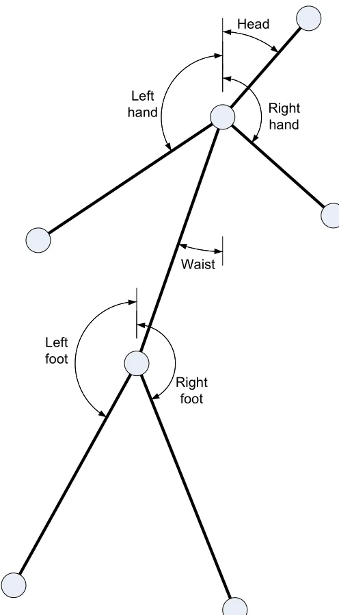
Figure 2: Single person body model with distance features labeled ... 19

Figure 3: Single person body model with angle features labeled ... 20

Figure 4: Person-object activity angle and distance features ... 21

Figure 5: Person-person activity distance feature ... 22

Figure 6: Background frame and frame 36 from subject 8's Standing video ... 23

Figure 7: Example 27 point Sukharev grid over HSV colorspace, from 3 views ... 24

Figure 8: Sample frame after background subtraction (Subject 8, Standing, frame 36) .. 25

Figure 9: Example frame for column density histogram (Subject 15, Approaching, frame 49) ... 26

Figure 10: Column density histogram for example frame shown in Figure 9 ... 27

Figure 11: Bounding box, left side, midline and right side (Subject 8, Standing, frame 36) ... 28

Figure 12: Example frame after pixel clustering (Subject 8, Standing, frame 36) ... 29

Figure 13: Example frame after merging pixel clusters into blobs (Subject 8, Standing, frame 36) ... 32

Figure 14: Example frame after skin labeling (Subject 8, Standing, frame 36) ... 33

Figure 15: Example frame after limb labeling (Subject 8, Standing, frame 36) ... 33

Figure 16: Example frame after feature extraction (Subject 8, Standing, frame 36) ... 34

Figure 17: Hierarchical body model for assigning blobs to limbs ... 35

Figure 18: Frame 36 of Subject 8's Standing video, with his hands in his pockets ... 44

Figure 19: Frame 63 of Subject 10's Jumping video, with his arms raised above his head ... 44

Figure 20: The static background scene ... 46

Figure 21: Example of noise around foreground edges (Subject 4, Jumping, frame 50) . 52 Figure 22: Example of disconnected feet (Subject 3, Jumping, frame 30) ... 53

Figure 23: Example of very poor background subtraction (Subject 10, Jumping, frame 63) ... 54

Figure 24: Example of shadow effects from ball on table (Subject 7, Picking Up, frame 15) ... 54

Figure 25: Example of oversegmentation in the legs (Subject 9, Waving Two, frame 40) ... 55

Figure 32: Example of good object segmentation during occlusion (Subject 7, Picking Up, frame 15) ... 60 Figure 33: Example of object not being found (Subject 2, Setting Down, frame 20) ... 60 Figure 34: Example of good feature identification in frontal view (Subject 11, Standing,

frame 61) ... 61 Figure 35: Example of good feature identification in side view (Subject 11, Walking,

frame 56) ... 62 Figure 36: Example of bad chest feature point extraction (Subject 9, Running, frame 32)

... 62 Figure 37: Example of bad chest feature point extraction (Subject 1, Waving Two, frame

26) ... 63 Figure 38: Example of good hand feature point extraction (Subject 1, Waving Two,

frames 2, 9, 14, 20) ... 64 Figure 39: Example of bad hand feature point extraction (Subject 3, Setting Down, frame

35) ... 65 Figure 40: Example of bad waist feature point extraction (Subject 12, Jumping, frame 25)

... 66 Figure 41: Example of bad feet feature point extraction (Subject 8, Running, frame 34) 66 Figure 42: Feature vector length distribution for vectors identified as single person

activities ... 67 Figure 43: Feature vector length distribution for vectors identified as person-person

activities ... 67 Figure 44: Feature vector length distribution for vectors identified as person-object

List of Tables

Table 1: Symbols used in Expectation Maximization equations ... 30

Table 2: List of features used ... 38

Table 3: Activities by activity type ... 42

Table 4: Activity types and descriptions ... 43

Table 5: Volunteers for the video database varied in height, ethnicity, gender, and clothing style ... 45

Table 6: Activity abbreviations used in classification tables ... 49

Table 7: Color codes used in classification tables ... 49

Table 8: Classifications for dataset videos, run over entire dataset ... 49

Table 9: Number of videos correctly and incorrectly classified, grouped by activity type ... 49

Table 10: Frame classifications for each activity, all dataset videos included ... 50

Table 11: Classifications for dataset videos, with poorly segmented videos excluded .... 50

Table 12: Number of videos correctly and incorrectly classified, grouped by activity type, with poorly segmented videos excluded ... 51

Chapter 1: Introduction

Automatic recognition of human activities in video is an increasingly active field of

computer vision research, spurred by significant demand in the military, security and

commercial sectors. Applications for this technology vary widely, ranging from

automated surveillance to home video gaming systems, presenting researchers with a

heterogeneous and sometimes conflicting set of requirements. As such many different

algorithms have been proposed and analyzed.

Many of these algorithms focus on identifying activities performed by a single

person in a scene. When multiple people are present, some algorithms examine the

movement of them in the scene, but not what each individual is doing. An algorithm

which can analyze several subjects in a scene, recognizing person and

person-object interactions in addition to single person activities would be a step closer to

advanced real-world applications of this technology. Current algorithms and techniques

are discussed in Chapter 2.

The objective of this thesis is to investigate the design of an algorithm using

limb-level features for identifying single-person activities, activities involving two people, and

activities between a person and an object. The methodology behind the algorithm’s

There were very few datasets available that were appropriate for objectively

measuring this algorithm’s performance. Existing datasets do not include the desired

activities or were recorded in such a way that they are unusable for this thesis. A new

dataset was created for this and future research. It consisted of fourteen volunteers

performing twelve activities in an indoor setting. More information on the dataset is

Chapter 2: Background

Activity recognition algorithms can be classified based on the type of activity they

recognize and the level of detail at which they operate [1]. There are algorithms which

can identify single-person activities [2], [3], multiple-person interactions [4], [5], [6], [7],

and person-object interactions [8], [7], [9]. Some infer a person’s actions by examining

their silhouette [2], [10], [11], [12], whereas others are able to distinguish between

actions based on individually-identified limbs [6]. A subclass of activity recognition,

gesture recognition, operates at a finer level of detail to recognize complex finger and

hand motions such as those used in sign language [13], [14].

There are many challenges that make human activity recognition difficult.

Depending on the environment, an algorithm may need to contend with changing lighting

conditions and dynamic shadows during segmentation. Movement unrelated to the

subject should not distract the recognition algorithm. Very often an algorithm must

perform temporal segmentation, i.e., determine when an activity begins and ends in a

continuous video stream [15], [16].

When identifying features of interest, occlusion is a major problem. Even in

single-person activity recognition with no obstructing foreground elements, the hand of a

computer analysis of human movement. The outlier cases of people using alternate

modes of transportation (e.g., inline skates or scooters), children, and people with

disabilities further complicate the matter. The heterogeneity of subjects is a significant

obstacle to deploying activity recognition algorithms in real-world applications.

Algorithms that identify human activities typically require several layers of

processing. They must segment the scene’s subjects from the background, identify

features of interest, and classify the activities being performed. The processing

techniques applied at each level are largely dependent on the types of activities being

classified and the target environment. For example, using background subtraction for

segmentation would not work well in an outdoor environment with swaying trees.

However it could perform very well indoors where the background is static.

Sometimes researchers ignore real-world issues such as real-time performance

and scalability when developing new algorithms. Certain algorithms can be trained to

recognize a set of core activities [2], [5]. This makes the algorithms application specific,

but it makes testing significantly easier. Algorithms using context-free grammars to

describe activities that are more easily extended to include new activities have been

explored recently [6].

An activity recognition algorithm could easily take several minutes to process a

The fact remains that automatic human activity recognition is a broad and

complex area of research. The wide range of approaches researchers take on the problem

is indicative of this. Any new research helps to advance the state-of-the-art by identifying

techniques to pursue and techniques to avoid.

2.1

Supporting work

There has been a large amount of research performed on single-person activity

recognition, but comparatively little on activity recognition in scenes with multiple

interacting persons, especially at the limb level of detail [17]. Yet it is often the case that

there are multiple persons in a surveillance camera’s field of view. Enabling existing

algorithms to recognize the activities of multiple non-interacting persons is relatively

simple, as it only requires a new tracking mechanism that can identify multiple targets

simultaneously. Identifying direct (e.g., shaking hands) and indirect (e.g., approaching

and departing) interactions, however, requires more infrastructure. New segmentation

algorithms and more detailed activity descriptions all must be developed for a system to

effectively recognize interactions.

There are several common techniques for segmenting persons from the

background in a video. Background subtraction is typically used in scenes with static

backgrounds due to its simplicity and low computational complexity. Motion-based

motion energy of a scene. This can potentially lead to over-segmentation due to small

fluctuations in limb velocities, but overall it seems to work very well. In [15] Rui and

Anandan use optical flow to detect temporal discontinuities as activity boundaries. A

much simpler technique is to label periods of time based on the dominant action, as in

[2]. This method places more emphasis on the subject’s pose rather than his movement,

and assumes that a recognizable activity is being performed during a particular time

frame. Though it is relatively imprecise for rapidly changing activities, it does provide a

general sense of what has occurred.

Occlusion can be handled several ways. In [20] Khan and Shah classify pixels in

each frame by determining which pixel cluster they belong to from a previous frame.

When pixels are occluded their cluster remains in memory, so that when they reappear

they are still assigned to the appropriate cluster. They also provide a method for detecting

when a new person has entered the scene. Other probabilistic approaches use an

appearance model to distinguish between multiple persons in a scene [21].

An increasing amount of research is being performed in using multiple cameras

for activity recognition. The availability of multiple viewpoints of a scene makes it much

easier to develop three dimensional models of the subject in the video. As a result, some

view-invariant algorithms have been developed [3]. The downside to volumetric

Activity recognition is still an emerging field and nearly all research has been

targeted at recognizing the actions of adults. The KidsRoom [22], an interactive

story-telling environment, was one application of coarse activity recognition with children.

Though it recognized some simple actions, such as crouching and making a “Y” with

their arms, it did not address the issue of tracking adults and children in the same scene.

This is a potential issue when working on identifying interaction activities.

J. K. Aggarwal at the University of Texas at Austin has performed a significant

amount of research in the field of activity recognition. He and his colleagues have

published papers on human segmentation, motion analysis, activity recognition [23] and

activity semantics, among other areas.

In [23] Park and Aggarwal describe an algorithm for the tracking and

segmentation of multiple persons in a scene. The algorithm is divided into several layers.

Background subtraction is applied followed by pixel-color classification. Blobs are then

formed, tracked, and eventually assigned to body parts. One key aspect of Park and

Aggarwal’s classification algorithm is its use of skin detection to help identify body parts.

It is a simple but effective method of increasing the algorithm’s accuracy.

Park and Aggarwal claim a 97% pixel classification accuracy, which is

comparable to other algorithms, but their work is not designed for real-time applications.

The pixel classification uses an iterative approach and takes a considerable amount of

event hierarchies [7]. Semantic descriptions are much closer to natural language

descriptions of activities and can provide more information to the user about what

occurred in a scene. Grammars provide an efficient, scalable method of creating these

descriptions through the application of a set of recursive rules. The development of

optimal grammars for activity recognition is an ongoing research effort.

Boeheim and Savakis developed a real-time single-person activity recognition

algorithm using feature point detection [2]. They used background subtraction to obtain a

thresholded silhouette of the person and skeletonized it. Using masks they identified

feature points, such as the head, hands, and feet, and constructed a six segment model of

the person. Finally they fed the locations of the feature points to an artificial neural

network for classification.

A logical extension to Boeheim’s algorithm would be to enable multiple-person

and person-object activity recognition, such that the system could identify activities from

any of the three activity types. The body model used in Boeheim’s work is easily

extendible to person-person and person-object activities. Park and Aggarwal [23]

achieved good segmentation performance with their background subtraction and pixel

clustering algorithms, so incorporating these into Boeheim’s algorithm could yield

improved classification accuracy. These techniques together are also potentially viable

Chapter 3: Methodology

The first steps in designing any computer algorithm are to identify the algorithm’s

primary task and to use functional decomposition to break it down into smaller tasks. An

algorithm for identifying the activities of humans in a scene must, at the highest level,

locate features of interest and use that information to classify the activities. Locating the

features of interest is the primary task the algorithm must perform, a task which can be

broken down into identifying the foreground, distinguishing between individuals in the

scene, segmenting them into body parts, and analyzing the segmented parts for the

feature coordinates.

Figure 1: The algorithm’s processing stages

can be passed between cores to maximize parallelism and overall throughput. The

following sections describe the algorithm in detail.

It is critical to consider the target environment when choosing techniques that

accomplish these tasks. This research was targeted at indoor environments, e.g. a room

with constant lighting, a static background and relatively little clutter. An assumption of a

fixed camera with frontal and side views of the subjects also greatly simplified the

algorithm’s design.

The representation of the subjects in a scene not only affects algorithm design but

is also a critical factor in determining the algorithm’s classification accuracy. A good

model will capture all of the relevant information in a scene; here that consists of the

subjects’ poses and movements. Simple five or six segment body models have been

shown to work well for representing most human activities [12]. A six-segment body

model was used, as in Boeheim’s work. It encodes the relative positions and movement

of the limbs and torso, the critical information for the activities being identified.

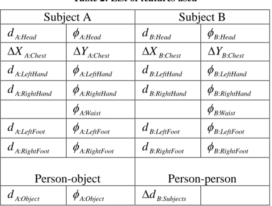
The feature vector derived from this model included the location of the head,

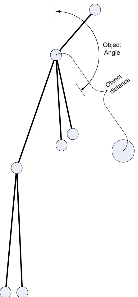
hands and waist relative to the chest, the location of the feet relative to the waist, the

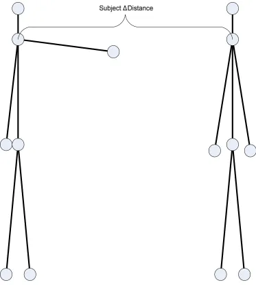
movement of the chest, the distance between the chest and the object (for person-object

activities), and the distance between subjects (for person-person activities). These

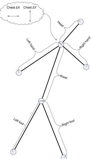
Left hand

Head

Right hand

Waist

Right foot Left

foot

Figure 5: Person-person activity distance feature

Prior to the main loop, the algorithm must initialize several models and starting

Figure 6: Background frame and frame 36 from subject 8's Standing video

The background model is generated by measuring the color of each pixel in an

empty scene, in the same manner as Ryoo and Aggarwal [7]. An example of an empty

scene is shown in Figure 6. A number of frames are examined and the mean and variance

of each pixel is calculated. Twenty frames generally provide enough information for

calculating these values. The Hue-Saturation-Value (HSV) was used to represent the

background because it maps naturally to human perception of color and performs better

for segmentation in later steps.

The skin and object models are simply parameters for classifying skin and objects

by color. The skin model was determined by manually labeling skin within the dataset

and determining the average HSV values. The object model parameters were obtained in

the same manner. These models are extremely simplistic but simple to implement and

surprisingly effective.

their values need to be modified whenever the algorithm is used on new video or in a new

environment.

The pixel clustering’s starting vectors must also be initialized before the

algorithm begins processing frames of video. Park and Aggarwal [23] used random initial

vectors for the Expectation Maximization algorithm, but this makes consistent

performance for testing difficult due to the fact that algorithm results are not repeatable.

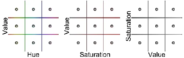
A Sukharev grid was used to determine the initial color vectors [24], depicted in Figure 7.

That is, a cubic grid of points evenly distributed throughout the HSV color space were

used as the vectors initially fed into the pixel clustering algorithm. This reduces the

possibility that a particular color is missed when the colors vectors converge.

Figure 7: Example 27 point Sukharev grid over HSV colorspace, from 3 views

When the number of vectors being initialized is not a perfect cube, the points are

initialized along the Hue axis first, as this is the most important color channel for

segmenting the human subjects. The second axis was Saturation, and then Value. The

segmenting a single subject, assuming two colors for the hair, skin, shirt, pants, shoes and

object regions.

3.2

Background Subtraction

Figure 8: Sample frame after background subtraction (Subject 8, Standing, frame 36)

After initialization, the algorithm enters the main loop. The first step after obtaining a

new frame from the input device is to extract the foreground, as shown in Figure 8. This

is accomplished by determining the Mahalanobis distance between the pixels in the

current frame and the background model [23].

(

)

(

)

= −

x S x

d T 1 (1)

The distance d is computed from the input pixel vector x, the pixel mean µ, and

the pixel covariance matrix S. If the distance is above a predetermined threshold the pixel

The next step after obtaining the foreground mask is to locate the individual

subjects in the scene, since the algorithm supports more than one subject.

3.3

Locating Subjects

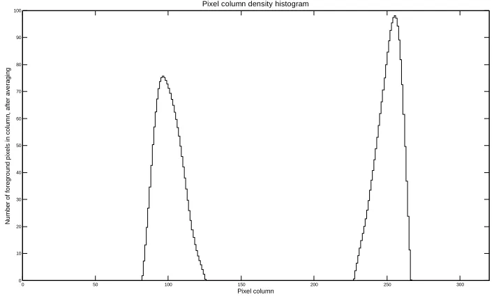
Locating the subjects in the scene is simply a matter of generating a histogram of column

densities in the mask and then finding the peaks [23]. The mask pixels in each column of

the image are summed, and the resulting vector is averaged. The averaging window was

chosen to be the estimated width of subjects in the scene, in order to produce a histogram

with a smooth derivative. Figure 9 and Figure 10 show what the histogram looks like for

a given foreground.

0 50 100 150 200 250 300 0 10 20 30 40 50 60 70 80 90 100 Pixel column N u m b e r o f fo re g ro u n d p ix e ls i n c o lu m n , a ft e r a v e ra g in g

Pixel column density histogram

Figure 10: Column density histogram for example frame shown in Figure 9

The peaks are thresholded to remove any noise, and the result is used to calculate

the left and right sides of the subjects’ bodies as well as their midlines. The algorithm

simply looks for where the peaks begin and end, and then chooses the maximum of the

peak as the midline.

Notice that the maxima are not centered within the peaks. This is beneficial for

calculating the subjects’ midline. Looking at the right subject in Figure 9 we see that her

foot is sticking out, skewing the centroid of her bounding box to the left. However with

the column density histogram we see that the maximum is located properly above her

midline.

The top and bottom of the subject were located in a similar manner to the left and

The divisions between the head and torso and then between the torso and legs are

based strictly on the height of the silhouette. In [23] Park and Aggarwal determined that a

human’s head is 16% of their height, and that their legs are 55% percent, providing

simple ways for estimating the neck and waist location. These bounds do move when the

subject puts their hands above their head, but the different is only a few pixels, so it does

not present a problem for the algorithm.

Figure 11: Bounding box, left side, midline and right side (Subject 8, Standing, frame 36)

The end result of the bounds calculation is shown in Figure 11. The far left and

far right bounds extend past the body to ensure that no part of the body is cut off during

segmentation. This is particularly important when the arms are extended outwards and

they are not clear in the column density histograms. In these cases the extra width ensures

3.4

Pixel clustering

Figure 12: Example frame after pixel clustering (Subject 8, Standing, frame 36)

At this point the algorithm processes each subject individually. The pixel clustering

portion of the algorithm groups foreground pixels into blobs based on color, with the goal

of segmenting the subject’s image into individual body parts, such as the head or hands.

Figure 12 shows a frame of video after pixel clustering.

In order to cluster pixels by color the algorithm must have a set of colors where it

will assign the pixels. Given that the primary colors in the foreground image are that of

the skin and clothing of the subjects, it is not possible to know beforehand what these

colors will be. The colors must be determined through an assumption. If we assume that

each color in the image has a probability distribution, we can determine the likelihood

that a pixel’s color belongs to ones of those distributions.

( )

∑

( )

( )

p ω ω (2)

( )

( )

(

)

(

)

1 2 1 2 ,..., 1 , 2 exp

2 v v r C

v

p r r

T r r

d

r  =

  



 − Σ −

− × Σ = − −

− µ µ

π

ω (3)

In Equation 3 p

( )

calculated from a simple d-dimensional Gaussian distribution. In Equation 2 p

( )

represents the overall color distribution of pixel v; it describes how likely the pixel v

belongs to any one of the color classes.

Expectation Maximization alternates between an Expectation step and a

Maximization step. Essentially the Expectation step calculates the probabilities of each

color class given the pixels in the image, and the Maximization step updates the colors to

maximize these probabilities. Eventually the color classes converge to values that

maximize the Prior probabilities.

Table 1: Symbols used in Expectation Maximization equations

Symbol Description

v Vector (representing 3 channel pixel)

0

C Number of color classes

( )

Pω Prior probability of the rth color classωr

r

Σ Covariance matrix of the rth color classω_r

r

µ Mean of the rth color classω_r

( )

p Probability of pixel v being the color it is given a set of color distributions

( )

(

)

(

(

)

( )

)

( )

∑

← _c

j k j j i i i i k k i P v p P v p v P 1 ˆ ˆ , ˆ ˆ , ˆ , ˆ ω θ ω ω θ ω θ ω (4)

The maximization step consists of updating parameters Pˆ

( )

i

Σˆ . These

are updated individually for each color classes i=1 C.. ₀. The new prior probability

( )

Pˆ ω for color class ωi is the average probability calculated in Equation 4 for all pixels

k

v . The new mean µˆ is the average color of all the pixels in the image weighted by the _i

normalized probabilities Pˆ

(

)

i

Σˆ is calculated in the same

manner as the mean.

( )

∑

(

)

i P v

n P 1 ˆ , ˆ 1

ˆ _{ω ω θ (5)}

(

)

(

)

∑

∑

k i k n

k i k k i v P v v P 1 1 ˆ , ˆ ˆ , ˆ ˆ θ ω θ ω µ (6)

(

)

(

)(

)

(

)

∑

∑

k i k n k T i k i k k i

i _{P v}

v v v P 1 1 ˆ , ˆ ˆ ˆ ˆ , ˆ ˆ θ ω µ µ θ ω (7)

A maximum a posteriori classifier is used to assign the pixels to each color class.

The class of each pixel is the class which maximizesP

( )

( )

(

)

L =argmax log ω , 1≤ ≤

ω (8)

Once the pixels have been assigned a known color, they are grouped by their

connectivity to neighboring pixels of the same color, forming blobs. Characteristics about

these blobs are calculated, including blob areas and blob neighbors. This information is

used to merge blobs together to form larger blobs, reducing noise and better representing

the underlying object. The algorithm loops through the list of blobs and finds blobs which

are smaller than a given threshold, measured as the area of the blob in pixels. The small

blobs are merged into the neighboring blob with the most shared perimeter. After

merging the blobs, a frame looks like Figure 13. After this merging is complete the

resulting blobs are characterized once again for use in later stages of the algorithm.

Figure 13: Example frame after merging pixel clusters into blobs (Subject 8, Standing, frame 36)

The blobs’ colors are analyzed and labeled as skin or non-skin. Figure 14 shows

Figure 14: Example frame after skin labeling (Subject 8, Standing, frame 36)

The area between the subject’s waist and knees is masked to reduce confusion

between the legs and the object in person-object activities. This does not impact the

feature extraction stage of the algorithm because it does not used any pixel information

from this region.

3.5

Feature point extraction

The features used to classify the activity being performed are extracted after blobs have

been formed. Figure 16 shows features marked with black dots with white outlines. The

right hand feature is missing.

Figure 16: Example frame after feature extraction (Subject 8, Standing, frame 36)

These features include the location of the head, the hands, the waist, and the feet.

These are all calculated in polar coordinates relative to the chest, the most stable feature

point. Distances are normalized by the distance between the chest and waist. The change

in location of the chest is also used. In person-person activities the change in distance

between the two subjects is used. In person-object activities the location of the object

relative to the chest is used.

of pixel rows. The torso region includes all blobs between the 16% and the 45% rows

from the top, while the leg region contains all the remaining blobs at the bottom of the

subject.

Figure 17: Hierarchical body model for assigning blobs to limbs

The torso region is then segmented into chest and arm regions, depending on

whether the blobs are labeled as skin or not.

At this point there is enough information to locate the chest feature. The torso

blobs are morphologically closed to remove holes and the largest blob is selected as the

chest. The centroid of this blob is used as the chest feature coordinates. The chest tends to

be the most stable feature point because it relies only on the existence of blobs in the

center of the subject’s silhouette. For this reason it was chosen as the root feature point

relative to the other feature points are calculated relative to.

skin blobs in the same area are called hair, and skin blobs outside of that area are arm

blobs. The centroid of all the face blobs is used as the face feature coordinates.

The legs are also segmenting into either hands or legs, again based on whether

they are skin or not. This makes it possible to identify the hands. The most difficult part

of locating the hands is determining how to classify the arm blobs as a left arm or right

arm. To do this, the algorithm first determines if the arm blobs are to the left side of the

body, to the right side, or over the middle of the body. The centroid of all the center arm

blobs is calculated, and assigned to the arm depending on which side of the subject’s

midline it is.

Next the left and right arms are examined individually. The arm blobs are

morphologically opened and closed to remove noise and false skin classification. The

largest blob is selected as the best arm or hand candidate, and its location is compared to

the location of the chest. If it is above the chest, the top-left or -right extreme is used. If it

is below, the bottom-left or -right is used. The extrema are calculated simply by

examining the outer column or row of pixels and then selecting the pixel at one end or the

other. For example the bottom-left extrema is found by selecting the left-most pixel in the

bottom row. This relatively simple calculation locates the hand quite well in both frontal

and side views of the subject.

The feet location algorithm is relatively simple. Blobs that were previously

grouped into the leg region are assigned to either the left or right groups. This is not the

subject’s left or right, but the side of the person from the camera’s view that the leg is on.

The blobs to the left of the legs centroid are considered to be part of the left leg, whereas

those to the right are considered part of the right leg. The leg is then morphologically

closed, and the bottom-left and left-bottom extrema are calculated (bottom-right and

right-bottom for the right leg). The extreme that is farthest from the centroid of the legs is

used as the foot location.

The object is located using center of the bounding box for the largest blob labeled

as the object. This is better than using the centroid because when the subject is holding

the object, his or her hand occludes a portion of the object, which distorts the centroid.

After all the feature points have been extracted in Euclidean pixel coordinates,

they are converted to polar coordinates. This representation better models the relation of

the features to each other. The head, waist and hands are all converted to be relative to

the chest. The feet are relative to the waist. All distances are normalized by the distance

between the chest and the waist, since it’s the most distance between the two most stable

feature points.

Table 2: List of features used

Subject A Subject B

Head A

d _: φ_A:Head d_B:Head φ_B:Head

Chest A X :

∆ ∆YA:Chest ∆XB:Chest ∆YB:Chest

LeftHand A

d : φA:LeftHand dB:LeftHand φB:LeftHand

RightHand A

d _: φ_A:RightHand d_B:RightHand φ_B:RightHand

Waist A:

φ φB:Waist

LeftFoot A

d _: φ_A:LeftFoot d_B:LeftFoot φ_B:LeftFoot

RightFoot A

d _: φ_A:RightFoot d_B:RightFoot φ_B:RightFoot

Person-object Person-person

Object A

d : φA:Object ∆dB:Subjects

Additional normalization is performed on the data in order to equalize the weights

of the various features during classification. The goal is for each feature’s expected value

to fall between 0 and 100. The maximum and minimum values for each feature are

measured over the entire dataset and then the features are normalized over those ranges.

Lastly, the angles features were weighted by a factor of 2 and the chest movement by a

factor of 1.5, as this tended to generate better classification results.

The atan2 function common in many mathematical libraries was used for some

calculations. It is defined as:

(

) (

)

X X

Waist Waist Chest Waist Chest

d = − + − (10)

      − − = Y Y X X Waist Chest Waist Chest Waist arctan φ (11)

(

)

1

− −

=

∆ _{X X}

Waist

Chest Chest Chest d

X (12)

(

)

1

− −

=

∆ _{Y Y}

Waist

Chest Chest Chest d

Y (13)

(

) (

)

1 Y Y X X Waist

Head Chest Head Chest Head

d

d = − + − (14)

      − − = Y Y X X Head Head Chest Head Chest arctan φ (15)

(

) (

)

1 Y Y X X Waist

LeftHand Chest LeftHand Chest LeftHand d

d = − + − (16)

(

)

LeftHand =arctan2 Chest −LeftHand ,Chest −LeftHand

φ (17)

(

) (

)

1 Y Y X X Waist

RightHand Chest RightHand Chest RightHand d

d = − + − (18)

(

)

RightHand =arctan2 Chest −RightHand ,Chest −RightHand

φ (19)

(

) (

)

1 Y Y X X Waist

LeftFoot Waist LeftFoot Waist LeftFoot d

d = − + − (20)

(

)

LeftFoot =arctan2 Waist −LeftFoot ,Waist −LeftFoot

φ (21)

(

) (

)

1

− +

1

− − =

∆d_Object d_Object d_Object

(

)

Object =arctan2 Chest −Object ,Chest −Object φ

1

− − =

∆φ_Object φ_Object φ_Object (25)

(

)

Waist

Subjects ChestA ChestB d

d = 1 −

1

− −

=

∆d_Subjects d_Subjects d_Subjects

(26)

Once all of the features have been extracted for a video, the change in distance

between the subjects and the motion of the subjects are calculated. The chest motion is

tracked frame to frame. This is important for distinguishing between the very similar

Standing and Jumping activities. The distance between the subjects is based on the

distance between their chest feature coordinates.

Features which disappear and reappear greatly reduce the number of features that

the algorithm can use during the classification stage. A simple feature history was

implemented to reduce the effects of this. If a feature is missing, the algorithm will search

up to 5 previous frames for the last known feature value. Since the activities studied here

are relatively slow moving, this is a good approximation of where the features are when

they are momentarily lost.

Overall the feature extraction algorithm is mostly location based. Skin and object

3.6

Activity classification

Once the feature vector has been extracted the algorithm uses a k-Nearest Neighbor

classifier to determine the activity. The activity classifier loads all of the extracted feature

data and each feature vector is labeled as a single person activity, person-person activity

or person-object activity. This determination is made by examining the available features

within each feature vector. A vector is labeled as a person-object vector if the object

location feature is not zero. The same applies for person-person activities, when the

second person feature vector is not zero. All other frames are put in the single person

activity group. Separating the feature vectors in this manner increases the activity

classifier’s accuracy by preventing it from attempting to match incompatible feature

vectors.

Each frame was classified by a plurality vote of the nearest k=3 neighboring

feature vectors in the dataset. Each frame of video for a particular activity counts as a

vote for that activity, and the video is labeled as the activity with the plurality of votes.

Several criteria were used to determine the confidence of each frame vote. The

first criterion was the number of features that could be compared between feature vectors.

If the two feature vectors did not share at least 10 features, the vote was thrown out. A

value of 10 was chosen since in most cases the algorithm is expected to extract the head,

chest, waist, and feet, a total of 10 features.

KNN is when there are no good matching frame candidates, in which case the frame

would be labeled as unclassifiable.

Another factor used to determine confidence was the distance between the nearest

neighbor and the second nearest neighbor. When this difference was above a certain

threshold then there was a high probability that the nearest neighbor was the correct

choice, so the frame was not classified by plurality vote, but by the nearest neighbor.

3.7

Video dataset

The video database consists of fourteen individuals performing twelve activities. A child

was also recorded performing the activities as a fifteenth subject for future work, and was

not included in this thesis’ analysis.

The database consists of three types of activities: single person, person-person and

person-object. In [25] Gavrila identified three sets of generic action verbs appropriate for

testing human activity recognition algorithms, divided into single-person actions,

interactions with objects, and interactions between two persons.

Twelve single person, person-person and person-object activities were identified

as simple, representative examples of common actions, as outlined in Table 3. Starred

activities indicate activities analyzed by Boeheim and Savakis. Table 4 contains detailed

Table 4: Activity types and descriptions

Activity Type Description

Standing Single person One subject stands facing the camera.

Jumping Single person One subject jumps in place facing the camera.

Walking Single person One subject walks across the camera’s field of view.

Running Single person One subject runs across the camera’s field of view.

Waving One Single person One subject stands facing the camera and waves one

hand.

Waving Two Single person One subject stands facing the camera and waves both

hands.

Pointing Person-person Two subjects face each other across the camera’s field

of view, and one subject points at another. Shaking Hands Person-person Two subjects stand facing each other across the

camera’s field of view and shake hands.

Approaching Person-person Two subjects walk toward each other across the

camera’s field of view.

Departing Person-person Two subjects walk away from each other across the

camera’s field of view.

Picking Up Person-object One standing subject picks up a designated object

from a table.

Setting Down Person-object One standing subject sets a designated object down on

a table.

The subjects were all given identical instructions on the activities to perform. In

general most subjects performed the activities in roughly the same manner, with varying

levels of enthusiasm, but there were some marked variations. Subject 8 performed the

Standing activity with his hands in his pockets, as shown in Figure 18, while all the

Figure 18: Frame 36 of Subject 8's Standing video, with his hands in his pockets

Most subjects also performed the Jumping activity with their arms at their sides.

When Subject 10 performed the Jumping activity he raised his arms above his head, as

shown in Figure 19.

Figure 19: Frame 63 of Subject 10's Jumping video, with his arms raised above his head

are provided in Table 5. The videos were filmed in a laboratory environment, with

constant lighting conditions and a static background. Background videos were obtained

immediately prior to each activity to enable later background subtraction. Each activity

was trimmed to start immediately before the subject began an activity, and stop

immediately after. The videos were resized to 320x240 pixels and stored in

uncompressed 24-bit RGB format. The total duration of the videos was 12020 frames

(401 seconds), excluding background sample frames.

Table 5: Volunteers for the video database varied in height, ethnicity, gender, and clothing style

1 2 3 4 5 6 7

Figure 20: The static background scene

Ten subjects varying in gender, skin color, and height perform the interactions in

front of a stationary camera. They are instructed to perform each activity based on a

simple predetermined description and possibly a demonstration. A red ball and table is

used in the person-object interactions.

3.8

Implementation

The algorithm was implemented using MATLAB. MATLAB provides an

extensive library of math and image processing functions, reducing the amount of

programming and debugging necessary for prototyping a complex algorithm. After the

algorithm was implemented, the algorithm was analyzed and problem areas were

Chapter 4: Results and Analysis

Algorithm verification was generally performed through visual inspection. The behaviors

of the background subtraction, pixel clustering and feature extraction stages were easily

determined by examining the resulting output. Problems such as high background noise,

oversegmentation, or improperly located feature points are difficult to quantify

automatically without ground truth images, which are in turn very labor intensive to

generate. Visual inspection was a reliable, rapid alternative for ensuring that the

algorithm was operating as intended.

The algorithm as a whole was tested by running it on the entire video dataset to

extract the feature vectors, and then feeding the vectors to a classifier. The classifier used

a leave-one-out scheme where all of the videos for the subject present in the currently

analyzed video are excluded from the dataset. This more accurately represents the

algorithm’s performance since the classifier does not have any a priori knowledge of the

subject whose activities it is identifying.

The overall classification accuracy of the algorithm was calculated as the number

of videos correctly identified out of the total number of videos analyzed. The percentage

of correctly identified frames was also calculated. This value is a better indication of how

bad segmentation, classification was performed on the remaining dataset to see what its

hypothetical performance would be had all the videos been segmented properly.

Due to poor initial classification performance, a great deal of time was spent

investigating sources of error. Individual stages of the algorithm were analyzed in depth

to determine where the algorithm was failing. Some areas were determined to be

limitations of the proposed algorithm, whereas others are potentially correctable. The

following sections describe the results in more detail and enumerate the problems and

possible solutions with the proposed algorithm.

4.1

Overall Performance

The algorithm identified 120 videos out of 168 correctly, for an overall classification

accuracy of 71%. The algorithm’s overall classification performance is summarized in

Table 8 through Table 13. Table 8 and Table 10 depict the classification per video in the

dataset. Correct classifications are highlighted in green, whereas incorrect classifications

are highlighted in red. The incorrect classifications are marked with the activity that the

videos were mistaken for. The count column marked with a pound sign (#) indicates the

number of correctly identified videos for a particular activity (row) or subject (column).

The percentage column marked with a percentage symbol (%) indicates the percentage of

the number of frames out of the total number of frames for an activity that were not

classified. The Total column lists the total number of frames in the dataset for each

activity.

Table 6: Activity abbreviations used in classification tables

Single Person Person-person Person-object

Activity Abbr. Activity Abbr. Activity Abbr.

Standing S Pointing P Picking Up PU

Jumping J Shaking Hands SH Setting Down SD

Walking W Approaching A

Running R Departing D

Waving One W1

Waving Two W2

Table 7: Color codes used in classification tables

Classifications Classification percentages

Meaning Correct Incorrect 0-39% 40-59% 60-79% 80-100%

Color

Table 8: Classifications for dataset videos, run over entire dataset

Subject

Activity 1 2 3 4 5 6 7 8 9 10 11 12 13 14 # %

Standing J J J J J PU J 7 50

Jumping R 13 93

Walking PU A 12 86

Running W W W W 10 71

Waving One S PU S 11 79

Waving Two J W1 R 11 79

Pointing A SH SH A A 9 64

Shaking Hands PU D 12 86

Approaching SH SH SH P P D 8 57

Departing PU 13 93

Picking Up SD SD SD SD 10 71

Setting Down PU PU PU PU PU PU PU PU PU PU 4 29

# 5 10 10 10 9 8 11 9 11 4 9 5 9 10 120

% 42 83 83 83 75 67 92 75 92 33 75 42 75 83 71

Table 10: Frame classifications for each activity, all dataset videos included S ta n d in g J u m p in g Wa lk in g R u n n in g Wa v in g O n e Wa v in g T w o P o in ti n g S h a k in g H a n d s A p p ro a ch in g D ep a rt in g P ic k in g U p S et ti n g D o w n

% U

n cl a ss if ie d T o ta l fr a m es

Standing 412 399 1 0 21 38 0 2 0 24 38 6 36 193 1134

Jumping 139 726 40 14 28 42 0 0 0 1 10 1 64 133 1134

Walking 22 57 395 57 8 5 0 0 0 5 14 2 44 330 895

Running 12 27 104 228 9 18 0 0 0 13 6 2 35 228 647

Waving One 174 66 5 0 730 42 0 2 0 2 43 0 64 70 1134

Waving Two 27 55 6 3 121 728 0 9 0 0 19 11 64 155 1134

Pointing 0 0 0 0 0 0 509 224 213 69 0 0 45 119 1134

Shaking Hands 0 0 0 0 0 0 28 723 14 134 60 20 64 155 1134

Approaching 0 0 1 5 0 0 97 163 284 136 0 0 31 235 921

Departing 3 6 2 18 1 0 54 62 85 574 15 11 60 121 952

Picking Up 15 23 5 6 23 19 0 7 0 3 325 162 44 154 742

Setting Down 5 23 1 3 10 40 0 3 0 0 304 221 27 202 812

Overall frame classification accuracy: 60

In order to determine how well the overall algorithm performs in the absence of

extremely poor segmentation, subjects 1, 10, and 12 were excluded from the dataset and

the classification algorithm was run once more. With these subjects removed the

algorithm identified 112 out of 132 videos correctly, an accuracy of 85%. The single

person and person-person videos were classified with accuracies of 91% and 93%,

respectively, while the person-object activities were only identified 50% of the time.

Table 11: Classifications for dataset videos, with poorly segmented videos excluded

Subject

Activity 1 2 3 4 5 6 7 8 9 10 11 12 13 14 # %

Standing J J J J 7 64

Jumping 11 100

Walking 11 100

Running W W 9 82

Table 12: Number of videos correctly and incorrectly classified, grouped by activity type, with poorly segmented videos excluded

Activity type Correct Incorrect Total Accuracy

Single person 60 6 66 91%

Person-person 41 3 44 93%

Person-object 11 11 22 50%

Overall 112 20 132 85%

Table 13: Frame classifications per activity, with poorly segmented videos excluded

S ta n d in g J u m p in g Wa lk in g R u n n in g Wa v in g O n e Wa v in g T w o P o in ti n g S h a k in g H a n d s A p p ro a ch in g D ep a rt in g P ic k in g U p S et ti n g D o w n

% U

n cl a ss if ie d T o ta l fr a m es

Standing 434 288 3 0 24 34 0 1 0 16 1 0 44 193 994

Jumping 131 659 30 1 20 32 0 0 0 3 0 2 65 133 1011

Walking 31 31 369 48 5 6 0 0 0 5 0 0 45 330 825

Running 10 14 73 209 9 9 0 0 0 28 1 0 36 228 581

Waving One 83 12 0 0 750 31 0 0 0 0 0 0 79 70 946

Waving Two 13 11 2 0 122 667 0 5 0 0 1 2 68 155 978

Pointing 0 0 0 0 0 0 572 14 139 21 0 0 66 119 865

Shaking Hands 0 0 0 0 0 0 5 616 42 42 0 0 72 155 860

Approaching 0 0 1 0 0 0 73 56 312 71 0 0 42 235 748

Departing 4 4 4 11 0 0 60 11 103 444 0 0 58 121 762

Picking Up 5 14 0 0 4 17 0 0 0 0 217 165 38 154 576

Setting Down 2 11 3 0 9 42 0 0 0 0 207 182 28 202 658

Overall frame classification accuracy: 70

The activity classification matrix (Table 11) makes it clear that the algorithm also

had trouble with the Standing, Picking Up, and Setting Down activities. These activities

were all classified correctly less than 65% of the time.

For the Standing activity the primary cause behind this low figure was the fact

that the only feature that is very different from Jumping is the vertical chest movement.

very easily make the movement invisible. This is a limitation of pose-based algorithms

when dealing with activities which are primarily distinguished by motion.

The difference between the Picking Up and Setting down activities are also

limited, with the chief difference being in the object features (angle and distance between

chest and object). However there was a much larger problem which lead to the failure to

identify these activities. The object classification portion of the code was unable to

reliably locate and track the object, so there was a significant loss of input data.

The overall performance of the algorithm is determined by the performance of

each of its parts. The following sections describe the results from each stage of the

algorithm in detail, with good and bad output from each.

4.2

Background Subtraction

The background subtraction stage performed sufficiently well. As with any basic

background subtraction algorithm, noise in the image presented difficulties. Although

morphological filtering eliminated this problem almost entirely, the edges around the

persons were not perfect. Figure 21 shows an example of the noise around the foreground

There was also the problem of the gray baseboard and marker tray present in the

dataset videos. The gray is a very neutral color and tends to blend into the foreground in

HSV space. Subject 3’s feet are disconnected in the frame of video in Figure 22.

Figure 22: Example of disconnected feet (Subject 3, Jumping, frame 30)

The end result is that most subjects’ feet are not connected to their main body

silhouettes. The rest of the algorithm was designed with this in mind—the body’s

foreground need not be entirely connected for the algorithm to work.

From the activity classification matrix it is clear that the algorithm performed

especially poorly on subjects 1, 10, and 12. Examination of the processed videos revealed

that these subjects were poorly segmented. In the case of subject 10 this was due to bad

Figure 23: Example of very poor background subtraction (Subject 10, Jumping, frame 63)

Unfortunately this is an inherent limitation to background subtraction. The

activity recognition algorithm cannot compensate for the loss of this much of the

silhouette.

Shadows also caused some issues during background subtraction. The shadow

detection code performed well enough to remove them in most cases, but it was not able

to remove all of them. The shadow from the ball on the table is quite clear in Figure 24.

Generally the shadows were not big enough to significantly impact the algorithm’s

4.3

Pixel clustering

In many situations the pixel clustering algorithm made grouped the foreground pixels as

desired. However there were some situations in which it performed very poorly. The

problems stem from either oversegmentation, as in Figure 25, or undersegmentation, as in

Figure 26.

Figure 26: Example of oversegmentation, clustered pixels on left and merged blobs on right (Subject 14, Walking, frame 45)

Ultimately these oversegmented blobs are simply grouped into larger segments

representing the torso or legs. However oversegmentation makes this grouping more

difficult and resource intensive.

In other situations the subjects’ images were undersegmented. At times the

Figure 27: Example of undersegmentation in the legs (Subject 5, Picking Up, frame 24)

The skin detection algorithm worked surprisingly well given its simplicity. Using

only some simple color bounds the algorithm was able to identify skin in most situations.

In situations where the skin algorithm failed, it failed rather spectacularly. In some

situations chest was identified as skin, causing the arms and possibly the head to be

grouped together into a single large skin blob. The algorithm was designed with clothed

subjects in mind, so this completely confused it. In other situations no skin was found at

all. Poor skin identification is the primary cause of bad segmentation in subjects 1 and

Figure 29: Example of good (blue) and bad (red) skin identification (Subject 10, Pointing, frame 31)

clustering, where the skin pixels are not clustered with the non-skin pixels. This is simply

shifting the skin/non-skin confusion from the pixel clustering to the skin identification

algorithm. It would be possible for the skin identification algorithm to label and remove a

significant portion of the subject’s silhouette, reducing the effectiveness of the pixel

clustering algorithm. The clustering is essentially divided between the skin identification

code and the explicit pixel clustering code. The decision was made to let the pixel

clustering algorithm do its work, and let the skin identification