1
Numerical optimization and experimental validation for a
1tidal turbine blade with leading-edge tubercles
23
Weichao Shi*1, Mehmet Atlar1, Rosemary Norman1, Batuhan Aktas1, Serkan Turkmen1
4 5
1 School of Marine Science and Technology, Newcastle University, UK
6 7 8
Corresponding Author:
9
Weichao Shi, [email protected]
10
School of Marine Science and Technology
11
Armstrong Building, Newcastle University
12
United Kingdom, NE1 7RU
13
Tel: 0044 (0)191 222 6726
14
Fax: 0044 (0)191 222 5491
2
Abstract: Recently the leading-edge tubercles on the pectoral fins of humpback whales have 17
attracted the attention of researchers who wish to exploit this feature in the design of turbine 18
blades to improve the blade performance. The main objective of this paper is therefore to make 19
a further investigation into this biomimetic design inspiration through a fundamental research 20
study involving a hydrofoil section, which represents a straightened tidal turbine blade, with 21
and without the leading-edge tubercles, using computational and experimental methods. 22
Firstly a computational study was conducted to optimise the design of the leading-edge 23
tubercles by using commercial CFD code, ANSYS-CFX. Based on this study the optimum 24
tubercle configuration for a tidal turbine blade with S814 foil cross-section was obtained and 25
investigated further. A 3D hydrofoil model, which represented a “straightened” tidal turbine 26
blade, was manufcatured and tested in the Emerson Cavitation Tunnel of Newcastle University 27
to investigate the effect of various tubercle options on the lift and drag characteristics of the 28
hydrofoil. The experiments involved taking force measurements using a 3-component balance 29
device and flow visualistion using a Particle Image Velocimetry (PIV) system. These tests 30
revealed that the leading-edge tubercles may have significant benefits on the hydrodynamic 31
performance of the hydrofoil in terms of an improved lift-to-drag ratio performance as well as 32
reducing the tip vortex which is main cause of the undesirable end-effect of 3D foils. The study 33
explores further potential benefits of the application of leading-edge tubercles on tidal turbine 34
blades. 35
Keywords: Tidal turbine, Leading-edge tubercle, Foil tests, Computational Fluid Dynamics 36
3
1
Introduction
38
The humpback whale is a species of giant marine mammal, ranging from 12~16m long. In spite 39
of its large size this creature is unique in its ability to do athletic manoeuvres, especially in 40
catching its prey, compared to other similarly sized marine mamals. Humpback whales utilize 41
their unusually long pectoral fins to perform tight turns to drive a school of fish into a small 42
circular zone so that they can swallow their prey all together. Close observation of their long 43
fins indicates that the leading edges of these fins are not smooth, having some tubercles which 44
are round shape protuberances [1, 2]. Wind tunnel tests showed that placing leading-edge 45
tubercles on foils could improve the foil performance in terms of delayed stall and higher lift-46
to-drag ratio [3-8]. 47
A number of numerical and experimental investigations has been conducted to understand the 48
tubercle concept [8-12]. Some of these investigations indicated that the effects caused by the 49
tubercles on the performance of a 2 dimensional (2D) foil and 3 dimensional (3D) foil are quite 50
different [3, 5, 6, 9, 11, 13-15]. Studies on the 2D foils were more focused on the optimisation 51
of the sinusoidal shape tubercle profiles defined by different parameters. Optimised tubercle 52
profiles on these 2D sections could improve the lift coefficient curves further by maintaining 53
the lift after the stall point. However this was at the cost of a reduction in the maximum lift 54
coefficients since the drag coefficients were increased by these tubercles, at the same time. On 55
the other hand, different performance characteristics have been reported based on the 56
investigations with the leading-edge tubercles on 3D foils which are usually tip tapered like 57
rudders, stabilizer fins, wings, flippers etc. The investigations with the 3D foils also claim the 58
improvement of the lift coefficient curves by maintaining the lift beyond the stall point which 59
is similar to the effect of tubercles on 2D foils. However, in addition to this, the performance 60
regarding to the lift-to-drag ratio can be enhanced [6-8, 11, 16, 17]. 61
Encouraged by the previous investigations into tubercle performance, especially for the 3D foil 62
applications, an attempt was made recently to apply the tubercle concept to tidal turbine blades 63
and scaled turbine models with different tubercle designs were tested in a towing tank [18]. 64
Some performance improvement was demonstrated in this application even though the power 65
coefficients achieved were not comparable to state-of-the-art levels due to various design and 66
other issues developed during the tests. The blade with only a 1/3 of the span covered with 67
tubercles displayed the best performance amongst the different ranges of the tubercle 68
extensions over the blade span. Based on the results of this recent research it was thought that, 69
there was a scope for further research and development in this field to improve the performance 70
of a tidal turbine and demonstrate it in a validated manner. 71
The main objective of this study is therefore to make a further contribution to the understanding 72
of the tubercle concept in the design of tidal turbine blades by using computational and 73
experimental approaches. Within this framework, a fundamental investigation using a single 74
2D and 3D blade configuration is presented in this study. This is intended to achieve some 75
basic understandings of the leading-edge tubercles on a straightened turbine blade prior to 76
applying them to the real blades of a whole tidal turbine. 77
In the remainder of this paper, an optimization study is presented in Section 2 to optimise the 78
main parameters of the leading-edge tubercles for a single blade with S814 cross-section profile 79
4
fitted with different sizes of tubercles was analysed to lead on to the design of a 3D foil with 81
tubercles. Then a straightened 3D foil based on a tidal turbine blade with the same chord length 82
distribution but with a constant pitch angle was designed by using the optimised tubercles and 83
a physical model based on this design was tested in a cavitation tunnel as presented and 84
discussed in Section 3 of the paper. Finally main conclusions obtained from the study are 85
presented in Section 4. 86
2
Tubercle Design and Optimization
87
2.1 Description of Tubercle Design 88
The design study was based on a previous UK National research programme (EPSRC-RNET), 89
in which a tidal turbine was designed based on the S814 profile cross-section from the NREL 90
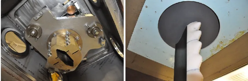
series, as shown in Figure 1 from Wang et al [19] who conducted an experimental investigation 91
into the efficiency, slipstream wash, cavitation and noise characteristics of this turbine. The 92
scaled turbine model is shown in Figure 2 as mounted on the open water dynamometer of the 93
Emerson Cavitation Tunnel of Newcastle Universiy. A representative and straightened version 94
of this turbine blade, which is based on the S814 profile cross-section, was considered as the 95
reference foil in this study to apply the tubercle concept. 96
The investigation into the optimisation of the tubercle profiles was initiated by systematically 97
changing the Height (H) and the Wavelength (W) of these protrusions based on the sinusoidal 98
form of their shapes. Two sets of tubercle designs were simulated with two different heights 99
which were assumed 5% and 10% of the foil chord length (C) and combined with ten 100
wavelength arrangements varying from 0.1C to 1C in 0.1C increments. The definitions of these 101
parameters are shown in Figure 3. 102
2.2 Numerical Method and Validation 103
Before investigating the effect of the designed tubercles on the foil performance, the foil test 104
data available from Ohio State University was used to validate the CFD model [20, 21]. 105
According to the previous 2D foil studies [5, 6, 8, 11], the tubercles were found to be beneficial 106
when the foil was under stall or near stall conditions. However the simulation of a foil 107
performance under stall conditions was a challenging case in CFD simulations [22, 23]. 108
Therefore the establishment of a reliable CFD model, in terms of the turbulence modelling, 109
effective mesh generation, etc., would be critical for the simulations as discussed in the next. 110
2.2.1 Turbulence Model 111
For the optimisation study presented here, a more computationally economical time 112
independent steady state RANS model was preferred. Industrially acknowledged and 113
recommended K-epsilon and Shear Stress Transport (SST) turbulence models were 114
investigated in the study [23]. 115
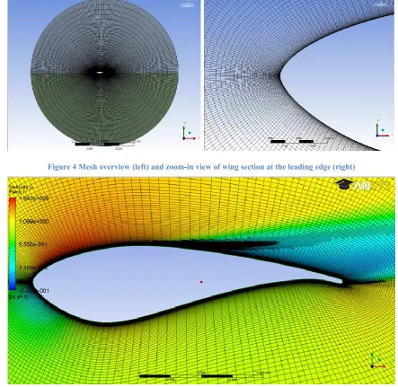
2.2.2 Mesh Generation 116
Mesh quality for curved surfaces is another critical issue for CFD simulations. As a first attempt 117
5
MESHING module [23]. The value of the non-dimensional wall parameter, y+, was kept as 1 119
to ensure the required mesh quality within the boundary layer [22] and the growth ratio was 120
limited to 1.08. The outer boundary was set at about 10 chord lengths away from the foil. 121
Meanwhile newly developed Solution Adaptive Mesh technology was also used to adapt the 122
mesh automatically based on the flow gradient [23]. This enabled more effective mesh 123
distribution depending on the requirements. 124
Figure 4 shows the whole mesh and the details of the grid near the foil section before the 125
solution adaptive mesh was processed. However after the process of solution mesh adaption, 126
the number of elements became around 2.5 million or more which depended on the calculation 127
cases. The mesh would be further refined automatically during the simulation itself, as shown 128
in Figure 5. 129
2.2.3 Validation of CFD 130
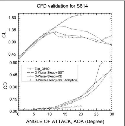
Figure 6 shows the comparison of the CFD predictions for the experimental lift and drag 131
coefficients of the Ohio State University foil. The CFD simulations were conducted using both 132
K-epsilon and SST turbulence models by maintaining the chord length based Reynolds number 133
at 106. As shown in Figure 6, both CFD simulations with the two different turbulence models 134
displayed very good agreement with the experiments up to a 10 deg of angle of attack (AOA) 135
where the stall occurred. After the stall, the CFD predictions overestimated the lift coefficient 136
especially using the K-epsilon turbulence model. However, when the CFD simulation with the 137
SST turbulence model was combined with the solution adaptive mesh technique [22] the 138
prediction was greatly improved, as shown in Figure 6. Similar comparisons are also shown 139
for the drag coefficients. As shown in Figure 6, the predictions with the SST turbulence model 140
combined with the solution adaptive technique show close agreement with the experimental 141
data. Finally, the comparisons of the CFD predictions with the experimentally measured 142
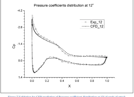
pressure distribution around the foil in stall condition are shown in Figure 7 and Figure 8 and 143
again display very good correlations. Therefore the SST turbulence model with the solution 144
adaptive mesh was adopted for the analysis of the flow. 145
2.3 Optimization Result and Analysis 146
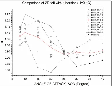
Using the validated CFD model, the lift coefficients of the foil with the S814 profile cross-147
section and sinusoidal tubercles of differing parameters were simulated. As shown in Figure 9 148
and Figure 10, the tubercles on 2D foils maintained higher lift coefficients in the post-stall 149
region (20o~40o) while they also reduced the maximum lift coefficient. Increasing the tubercle 150
wavelengths brought the lift coefficients of the foil with the leading-edge tubercles closer to 151
the lift coefficients of the reference or “baseline” foil with the smooth leading edge i.e. without 152
tubercles. However reducing the wavelengths increased the lift at higher angles of attacks while 153
reducing the maximum value of the lift. By taking into account these trends, the foil having a 154
sinusoidal form of tubercle with the height and wavelength of H=0.1C and W=0.5C, 155
respectively, was considered to be a good compromise from the performance point of view and 156
was chosen for further analysis as a 3D foil. 157
Post analysis of the CFD simulation results of the cases, “Baseline” and the optimised “H-0.1, 158
W-0.5”, under 15o are shown in Figure 11. The velocity iso-surfaces for the case where the 159
velocity is equal to 50% of the incoming velocity, reveal the flow separation patterns and were 160
6
around the foil was favourably affected by the presence of the tubercles as the flow appeared 162
to be more attached to the foil surface following the crest of the tubercles whereas the baseline 163
foil without tubercles displayed separated flow after the leading edge. 164
3
Foil Design and Test
165Having conducted the CFD analysis on the 2D foil and validated the results, the next task was 166
the design of a representative 3D foil with tubercles, based on an existing tidal turbine blade, 167
and to conduct dedicated experiments to investigate the effect of tubercles on the hydrodynamic 168
characteristics of this foil. 169
3.1 Foil Design and Manufacture 170
As reported in the open literature [6, 11] by previous researchers the effect of tubercles on the 171
hydrodynamic performance of 2D and 3D foils was different and further evidence supporting 172
this claim would be welcome as one of the natural outcomes of the present study. Therefore a 173
3D foil representing a turbine blade was designed and model tested in this section. 174
As stated in Section 2.1, the representative 3D foil was based on the blade of the tidal turbine 175
designed by Wang et al [19]. However, while the foil had the same chord length distribution 176
as the subject tidal turbine blade it had a constant pitch. Based on the limitations imposed by 177
the testing section of the ECT, the span of the test foil was specified as 560mm. Considering 178
the operating range of the tip speed ratios (TSRs), the range of the angles of attack (AOA) to 179
be applied on the foil during the tests was specified to be 0o to 40o while the inflow velocities 180
were selected as 2, 3 and 4m/s. Over this inflow velocity range, the reference Reynolds number 181
(Re), which was described based on the chord length (150mm) of the foil at 0.7 radius, was 182
varied from 0.3x10⁶ to 0.6x10⁶. This was similar to the Re range for the turbine model that was 183
used by Wang et al [19]. 184
According to the optimisation task with the 2D foil presented in Section 2.3, the foil with the 185
tubercles would display relatively the best performance when the height (H) and wavelength 186
(W) of the tubercles were 0.1C and 0.5C, respectively. Hence approximately 8 sinusoidal 187
tubercles with successive crests and troughs were evenly distributed along the leading edge. 188
Based on the above arrangement, the 3D foil was manufactured in two separate parts and then 189
assembled. The first part was the interchangeable (or removable) leading-edge part of the foil 190
while the second part was the remainder (i.e. main body) of the foil that also supported the 191
whole foil structure. The interchangeable leading-edge was printed using a 3D printer in four 192
segmented pieces from a liquid resin material, Stratasys Vero White Plus RGD835. 193
The interchangeable and segmented manufacture of the leading-edge profiles provided very 194
useful flexibility for testing the different leading-edge arrangements as well as overcomed the 195
size limitation of the 3D printer. The main body of the foil was milled by CNC machine from 196
a carbon fibre reinforced plastic (CFRP) to ensure that the structure would be strong enough 197
and the deformation minimal. All the models with various combinations of the leading edge 198
7
The main foil with five different leading-edge combinations, one of which was the smooth 200
leading edge, was tested and corresponding hydrodynamic performances were compared to 201
explore the effect of the four different tubercle arrangements on the foil performance. In order 202
to classify the different leading-edge tubercle combinations, the reference foil with the smooth 203
leading-edge section was represented by legend “0000” while the foil with the leading-edge 204
tubercles covering the whole span was represented by “1111”. Other leading-edge 205
combinations with partial tubercle applications were represented using legend “0001”, “0011” 206
and “0111” for the1/4, 1/2 and 3/4 coverage of the foil span by the tubercles from tip to root, 207
respectively. 208
3.2 Experimental Setup 209
The experiments were conducted in the Emerson Cavitation Tunnel (ECT) at Newcastle 210
University. The tunnel is a medium size propeller cavitation tunnel with a measuring section 211
of 1219mm×806mm (width × height), as shown in Figure 13. The speed of the tunnel inflow 212
varies between 0.5 to 8 m/s. Full details of the ECT and its further specifications can be found 213
in reference [24]. 214
The lift and drag performance of the test foil was the primary interest during the experiments 215
as in many foil investigations. During the tests, the forces (X, Y) acting on the foil, which was 216
suspended vertically from the upper lid in the mid-plane of the tunnel measuring section, were 217
measured using a 3-component balance device. This device was a Cussons R102 balance which 218
was specially designed and manufactured for the ECT to be mounted on the top lid of the tunnel 219
using a height and angle adjustment mechanism. The test foil was mounted to the bottom plate 220
of the 3-component balance to transfer the forces to the 3 load cells and a circular plate was 221
fitted at the root of the blade to prevent the tunnel inflow entering into the cavity, where the 222
balance was housed, as shown in Figure 14. 223
The measured lift and drag forces were represented by the following non-dimensional 224
coefficients: 225
𝐶𝐿 = 1𝐿𝑖𝑓𝑡 2 𝜌𝑉2𝐴
Equation (1)
𝐶𝐷 =1𝐷𝑟𝑎𝑔 2 𝜌𝑉2𝐴
Equation (2)
Where Lift is the measured lift of the foil which is perpendicular to the incoming flow; Drag is 226
the measured drag of the foil which is aligned with the incoming flow; 𝜌 is the density of the 227
tunnel water, which was measured as 1004 kg/m3 using a density meter; V is the tunnel inflow 228
velocity; A is the reference area of the foil which is assumed to be equal to the foil projected 229
area, 0.0924 m2. 230
All the measured data were gathered by a National Instruments data acquisition system and 231
8
acquired at a 1 kHz sample rate and averaged to calculate the mean value. During the 233
experiments, each test run was repeated three times for uncertainty analysis. The average 234
results were then plotted and compared. The maximum values of CL and CD were 2.3% and 235
3.1%, respectively, with mean values of standard deviation of 1.1% and 1.0%, respectively. 236
One example of the uncertainty analysis is presented in Figure 15. 237
In order to measure and analyse the flow field around the foil, a 2D particle image velocimetry 238
(PIV) system was used, while some still photo images were also taken. The detailed technical 239
specification of the PIV system used, which was a Dantec Dynamics Ltd product, is shown in 240
Table 2. During the use of this system, the flow field was illuminated by the planar laser light 241
sheet which was perpendicular to the hydrofoil and highly seeded flow field images were 242
captured by the double framing high-speed CCD camera at a frequency of 500Hz and 0.0004s 243
time interval. Throughout the measurements, 100 double frame image pairs needed to be 244
captured, analysed and averaged to achieve a time-averaged velocity distribution. The adaptive 245
PIV analysis was used for the 2D images from each camera with a grid size of 16x16 pixels. 246
Afterwards, the results of these 100 velocity samples were averaged to achieve the final results. 247
3.3 Force Measurement Results and Analysis 248
3.3.1 Reynolds Number Effect 249
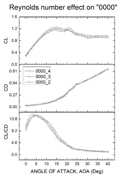
First of all, based on the above test set-up, the reference foil “0000” was tested at 2, 3 and 4m/s 250
tunnel velocity to demonstrate the effect of Reynolds number (Re). Because of the practical 251
limitations of the testing facility, a typical full-scale Re range for a tidal turbine, which often 252
ranges from 10x106 to 30x106 based on the chord length at 0.7 radius, could not easily be met 253
within the model scale test. In the current tests, the Re range was varied from 0.3x10⁶ to 0.6x10⁶ 254
where the Re was described based on the reference chord length of 150mm at 0.7 radius. It is 255
important that the Reynolds number effect has to be checked prior to any flow tests and certain 256
precautions must be taken to improve the circumstances for very low Re cases. 257
Figure 16 shows the measured lift, drag and lift-to-drag ratio of the reference foil (i.e. Foil 258
0000) which are represented in terms of the associated coefficients as described in Section 3.2. 259
In this figure the last character with an underscore bar in the legend used refers to the tunnel 260
incoming velocity (e.g. 0000_2, where the tunnel velocity is 2 m/s). As shown in Figure 16, 261
within the range of the Reynolds numbers tested, the slope and maximum value of lift 262
coefficients decrease gradually with increasing Re. On the other hand, the drag coefficients are 263
nearly identical for different values of Reynolds number. Thus, the lift-to-drag ratios of the 264
reference foil with the smooth leading-edge are reduced with increasing Reynolds number. 265
The tests conducted for the reference foil (Foil “0000”) were repeated for Foil “1111” which 266
had full leading-edge tubercles and the results are presented in Figure 17. As shown in Figure 267
17, unlike in the reference foil case, the lift coefficient of the foil with the leading-edge 268
tubercles increases with the Reynolds number, particularly after a 14o angle of attack (AOA) 269
for 2m/s and 3m/s flow speed. A large gap can be seen between the lift coefficients for 2m/s 270
and 3m/s. There seemed to be a trend suggesting that the lift-to-drag ratio can be enhanced with 271
increasing Reynolds number and hence the foil with the leading-edge tubercles may have a 272
9
3.3.2 Performance Comparison between the Foils with and without Tubercles 274
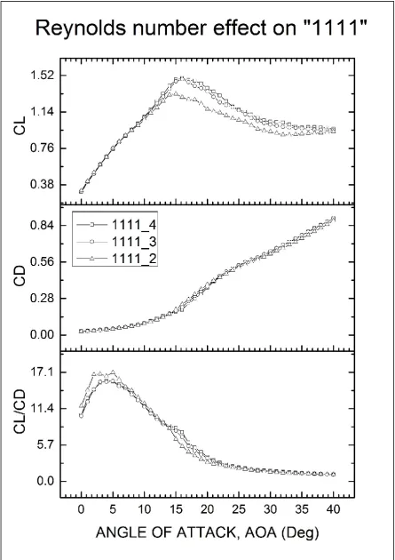
Figure 18 shows the comparison of the lift and drag performances for the reference foil (Foil 275
“0000”) and its counterpart (Foil “1111”) with a full set of leading-edge tubercles, at a 4m/s 276
inflow velocity which corresponds to the highest Reynolds number that was achieved. Figure 277
18 clearly shows the beneficial effect of the tubercles on the lift coefficient and hence on the 278
lift-to-drag ratios. It is interesting to note in Figure 18 that the lift coefficients of both foils are 279
almost identical up to an angle of attack (AOA) of 9-10o after which Foil “1111” can maintain 280
a linear growth until 16o AOA while Foil “0000” cannot. This results in a 32% increase of the 281
lift-to-drag ratio for the foil with leading-edge tubercles compared to the reference foil, as 282
shown in Figure 19. Meanwhile the peak lift-to-drag ratio of Foil “1111” also shows a 5.8% 283
higher value at 4o AOA. From Figure 19, it is clear that the enhancement caused by the leading-284
edge tubercles can be observed over the majority of the range of AOAs tested. 285
3.3.3 Performance Tests with Different Tubercle Coverage Arrangements 286
Although the beneficial effect of leading-edge tubercles covering the whole span of the foil has 287
been confirmed in the previous section, it has been reported in other research that this effect 288
may vary depending on the position and extent of the tubercles’ coverage relative to the foil 289
span [18]. Therefore 3 different tubercle coverage arrangements, which were described in 290
Section 3.1 as Foil “0001”, “0011”, “0111”, were tested to identify the optimum arrangement. 291
Five sets of tests, which also included the reference foil (“0000”) and the foil with full coverage 292
of tubercles (“1111”), were conducted at 3m/s and the results were compared, as shown in 293
Figure 20 to Figure 22. From the plots of the lift coefficients, it can be seen that the peak lift 294
coefficient tends to increase with the extent of the tubercles. As shown in Figure 20, Foil 295
“1111”, demonstrates the highest lift with a value of 1.48 at 16o AOA. Nevertheless this 296
arrangement also displays the highest drag. Based on the comparisons of the lift-to-drag ratios 297
of the tested arrangements, it appears that Foil “0001”, which had 1/4 of its leading-edge 298
covered with tubercles, displayed an overall better performance. This can be clearly seen in 299
Figure 21 and Figure 22 where Foil “0001” shows a positive impact from 0o to 26o AOA with 300
more than 10% enhancement in the maximum lift-to-drag ratio at 5o AOA, compared to the 301
reference (Foil “0000”). Even though Foil “1111” displayed the highest growth rate at 16o AOA, 302
Foil “0001” may offer more potential in improving the performance of a tidal turbine operating 303
over a wider range of tip speed ratios. 304
3.4 Flow Visualization Results and Analysis 305
3.4.1 Mapping the Flow Separation Region 306
Flow visualization tests with Foil “0000” and Foil “1111” were performed at a 3 m/s tunnel 307
inflow speed and at AOAs of 16o and 24o. For these conditions, the flow fields across three 308
selected sections along the foil span were visualised using the PIV device. The locations of the 309
selected sections are shown in Figure 23 for Foil “1111” and these positions were repeated for 310
Foil “0000”. For each test condition, 100 pairs of PIV images were analysed and averaged to 311
achieve the time-averaged data. The images of the flow fields and associated velocity vectors 312
at the three selected sections are shown in Table 3 and Table 4 for the AOA of 16o and 24o, 313
10
Firstly, concentrating on the 16o AOA results in Table 3, as shown in the first column (Section1) 315
the flow separation observed at the back of Foil “1111” is much stronger than the separation 316
observed at the back of Foil “0000”. As the visualisation sections are getting closer to the foil 317
tip the flow separation gradually vanishes as shown in the flow field results for “Section2” and 318
“Section3”. This can be related to the strong rolling up effect of the tip vortex forming from 319
the pressure side to the suction side of the foil which would reduce the flow separation. In fact, 320
hardly any flow separation could be observed from the results of “Section2” and “Section3” 321
with Foil “0000”. 322
On the other hand, as shown in Table 4, the results of the flow visualisations at 24o AOA 323
indicate severe flow separation for both foils. However the separation experienced by Foil 324
“1111” was even more severe than that experienced by Foil “0000”. 325
3.4.2 Development of Tip Vortex Cavitation 326
Perhaps the most striking difference between the flow pattern around Foil “0000” and Foil 327
“1111”, was the development of a very strong tip vortex cavitation generated by Foil “0000” 328
as opposed to almost no such cavitation generated by Foil “1111” due to the effect of the 329
leading-edge tubercles. This can be clearly seen in the results given in Table 3 for the test 330
condition with a 3m/s incoming velocity and 16o AOA. A close-upof this cavitating vortex, 331
which emanated from the tip of the reference foil with about a 10mm diameter, is shown in 332
Figure 24. 333
Using a typical cavitating Rankine vortex expression, the relationship between the diameter of 334
the cavitating tip vortex, 𝑎𝑐, and its circulation, Γ, can be given by Equation 3 [25].
335
𝑝∞− 𝑝𝑣 =
0.5𝜌Γ2 4𝜋2𝑎
𝑐 2
Equation (3)
where, 𝑝∞is the pressure in far field and 𝑝𝑣 is the saturated vapour pressure of the water. 336
According to Equation 3, the larger the diameter is, the stronger the vorticity. Since both foils 337
were tested under the same conditions, the larger tip vortex cavitation experienced by the 338
reference foil would be responsible for the stronger “end effect” and hence greater loss of lift. 339
whereas its counterpart (Foil “1111”) with the leading-edge tubercles would maintain the 2D 340
flow by lowering the end effect and therefore experience more favourable lift characteristics 341
for the same condition. 342
3.4.3 Concluding Remarks on the Effect of Leading-Edge Tubercles 343
Based on the observations and analyses so far, by combining our understandings from the flow 344
analysis with regard to the effect of different grades of flow separation and that of tip cavitation 345
generation with and without leading-edge tubercles, we can conclude that the leading-edge 346
tubercles can effectively weaken the 3 dimensional effect of the hydrofoil. 347
This hypothesis has been firstly supported by the evidence of much weaker separations 348
observed on the back of the reference foil with the smooth leading edge compared to the much 349
11
the measuring sections are very close to the tip, the 3D effect generates the rolling up flow 351
which can reduce the flow separation close to the tip region. Therefore the more severe the 352
flow separation at the tip region is, the weaker the 3D effect is. 353
On the other hand the hypothesis was also complemented by the evidence of suppressed tip 354
vortex cavitation and hence much reduced vortex strength resulting from the leading-edge 355
tubercles. This also supported that the 3D effect was weakened by the leading-edge tubercles. 356
4
Conclusions
357This paper reports research into the design, optimization and validation of a tidal turbine blade 358
to exploit the potential benefits of biomimetics in the form of leading-edge tubercles. Based on 359
the research so far, the following conclusions can be drawn: 360
1. As demonstrated in the optimisation study based on the 2D foil, while the application 361
of leading-edge tubercles could maintain high lift coefficients under post-stall 362
conditions, it could also lower the magnitude of the maximum lift. Based on the 363
optimisation study, a sinusoidal form of leading-edge tubercle profile with 0.1C height 364
and 0.5C wavelength appeared to be a good compromise for an optimum design and 365
this was applied on a 3D foil which was model tested to validate its performance. 366
2. Comparative model tests of the 3D foil with a smooth leading edge (no tubercles) and 367
with the leading tubercles, which covered the whole span of the foil, confirmed the 368
significant benefits of the tubercles on the lift and lift-to-drag ratio of the foil despite a 369
slight increase in the drag characteristics. A maximum improvement of 32% in CL/CD 370
can be gained in the post stall region at a 16o of angle of attack due to the linear increase 371
of the lift coefficient maintained with the increase of the angle of attack. 372
3. By optimising the application length of the leading-edge tubercles along the foil span, 373
it was found that the maximum lift coefficient was reduced with the reduced tubercle 374
application length. However, due to the enhanced lift coefficients before the stall and 375
compromised increase in the drag coefficient, the foil with the shortest tubercle 376
application length, which was equal to a 1/4 of the span, at the tip region displayed the 377
best overall performance amongst the different combinations tested. This was based on 378
the increased lift-to-drag coefficient ratio over the wider range of angles of attack and 379
more than 10% increase in the peak lift-to-drag ratio. 380
4. The flow visualisations of the 3D foil with and without the leading-edge tubercles 381
indicated that the strong tip vortex caused by the well-known end effect can be reduced 382
dramatically by the application of the tubercles which maintain the 2 dimensional 383
characteristics of the flow around the 3D foil. 384
Based on this research, the biomimetic exploitation of tubercles on tidal turbine blades has been 385
shown to be promising. However further fundamental research investigating the tubercle 386
12
Acknowledgments
388
This research is funded by the School of Marine Science and Technology, Newcastle 389
University and China Scholarship Council. Hence the financial support obtained from both 390
establishments is gratefully acknowledged. The Authors would like to thank all the team 391
members in the Emerson Cavitation Tunnel for the help in testing and sharing their knowledge. 392
Reference
393[1] F.E. Fish, P.W. Weber, M.M. Murray, L.E. Howle, The tubercles on humpback whales'
394
flippers: application of bio-inspired technology, Integrative and comparative biology, 51 (2011)
395
203-213.
396
[2] Frank E. Fish, J.M. Battle, Hydrodynamic design of the humpback whale flipper, Journal of
397
Morphology, (1996).
398
[3] K. L. Hansen, R. M. Kelso, B.B. Dally, The effect of leading edge tubercle geometry on the
399
performance of different airfoils, (2009).
400
[4] H.S. Yoon, P.A. Hung, J.H. Jung, M.C. Kim, Effect of the wavy leading edge on hydrodynamic
401
characteristics for flow around low aspect ratio wing, Computers & Fluids, 49 (2011) 276-289.
402
[5] H. Johari, C. Henoch, D. Custodio, A. Levshin, Effects of leading-edge protuberances on
403
airfoil performance, Aiaa J, 45 (2007) 2634-2642.
404
[6] D.S. Miklosovic, M.M. Murray, L.E. Howle, Experimental evaluation of sinusoidal leading
405
edges, J Aircraft, 44 (2007) 1404-1408.
406
[7] M.J. Stanway, Hydrodynamic effects of leading-edge tubercles on control surfaces and in
407
flapping foil propulsion, in, Massachusetts Institute of Technology, 2008.
408
[8] P.W. Weber, L.E. Howle, M.M. Murray, Lift, drag, and cavitation onset on rudders with
409
leading-edge tubercles, Mar Technol Sname N, 47 (2010) 27-36.
410
[9] A. Corsini, G. Delibra, A.G. Sheard, On the role of leading-edge bumps in the control of stall
411
onset in axial fan blades, J Fluid Eng-T Asme, 135 (2013) 081104-081104.
412
[10] T. Swanson, K.M. Isaac, Biologically Inspired Wing Leading Edge for Enhanced Wind
413
Turbine and Aircraft Performance, in, AIAA, 2011.
414
[11] E. van Nierop, S. Alben, M. Brenner, How bumps on whale flippers delay stall: An
415
aerodynamic model, Physical Review Letters, 100 (2008).
416
[12] L. Bellequant, L.E. Howle, Whalepower wenvor blade, (2009).
417
[13] K.L. Hansen, R.M. Kelso, B.B. Dally, Performance variations of leading-edge tubercles for
418
distinct airfoil profiles, Aiaa J, 49 (2011) 185-194.
13
[14] D.C.a.L.M. Mark W. Lohry, Characterization and Design of Tubercle Leading-Edge Wings,
420
in: Seventh International Conference on Computational Fluid Dynamics (ICCFD7), Big Island,
421
Hawaii, 2012.
422
[15] J.H. Chen, S.S. Li, V.T. Nguyen, The effect of leading edge protuberances on the
423
performance of small aspect ratio foils.
424
[16] G. Sisinni, D. Pietrogiacomi, G.P. Romano, Biomimetic wings, Advances in Science and
425
Technology, 84 (2012) 72-77.
426
[17] D.S. Miklosovic, M.M. Murray, L.E. Howle, F.E. Fish, Leading-edge tubercles delay stall on
427
humpback whale (Megaptera novaeangliae) flippers, Phys Fluids, 16 (2004) L39-L42.
428
[18] T. Gruber, M.M. Murray, D.W. Fredriksson, Effect of humpback whale inspired tubercles
429
on marine tidal turbine blades, in: ASME 2011 International Mechanical Engineering Congress
430
and Exposition, American Society of Mechanical Engineers, 2011, pp. 851-857.
431
[19] D. Wang, M. Atlar, R. Sampson, An experimental investigation on cavitation, noise, and
432
slipstream characteristics of ocean stream turbines, Proceedings of the Institution of
433
Mechanical Engineers, Part A: Journal of Power and Energy, 221 (2007) 219-231.
434
[20] D.M. Somers, Design and experimental results for the S814 airfoil, in, National Renewable
435
Energy Laboratory, NREL/SR-440-6919 • UC Category: 1213 • DE97000104, 1997.
436
[21] J. Janiszewska, R.R. Ramsay, M. Hoffmann, G. Gregorek, Effects of grit roughness and
437
pitch oscillations on the S814 airfoil, in, National Renewable Energy Lab., Golden, CO (United
438
States), 1996.
439
[22] F. Menter, M. Kuntz, R. Langtry, Ten years of industrial experience with the SST
440
turbulence model, Turbulence, heat and mass transfer, 4 (2003) 625-632.
441
[23] ANSYS, Release 14.5 Documentation, Inc ANSYS, (2013).
442
[24] M. Atlar, Recent upgrading of marine testing facilities at Newcastle University, in:
443
AMT’11, the second international conference on advanced model measurement technology
444
for the EU maritime industry, 2011, pp. 4-6.
445
[25] J.B.W. McCormick, On Cavitation Produced by a Vortex Trailing From a Lifting Surface,
446
Journal of Fluids Engineering, 84 (1962) 369-378.
14 449
Figure 1 Cross-section profile of S814 [19] 450
[image:14.595.87.498.70.518.2]451
Figure 2 Scaled tidal turbine model mounted on the dynamometer of Emerson Cavitation Tunnel [19] 452
[image:14.595.117.482.523.724.2]453
15 455
Figure 4 Mesh overview (left) and zoom-in view of wing section at the leading edge (right) 456
457
Figure 5 Refined mesh by the “solution adaptive mesh” method
16 459
17 461
Figure 7 Validation for CFD prediction of Pressure coefficient distribution at 12o of angle of attack
462
[image:17.595.77.514.353.695.2]463
Figure 8 Validation for CFD prediction of Pressure coefficient distribution at 15o of angle of attack
18 465
Figure 9 Comparison of 2D foil lift coefficients with different tubercle profiles by varying the wavelength (W) 466
at constant tubercle height (H=0.05C) 467
468
Figure 10 Comparison of 2D foil lift coefficients with different tubercle profiles by varying the wavelength (W) 469
[image:18.595.102.495.408.707.2]19 471
[image:19.595.68.529.90.229.2]472
Figure 11 Comparison of flow separation at 15o angle of attack (Velocity isosurface at 50% of incoming velocity
473
coloured by pressure distribution) 474
[image:19.595.69.528.261.450.2]475
Figure 12 Tested 3D hydrofoil models with interchangeable leading-edge parts 476
[image:19.595.64.502.339.713.2]477
20
[image:20.595.82.511.72.212.2]479
Figure 14 Setup of 3-component balance (Cussons R102) on the Emerson Cavitation Tunnel upper lid (Left) and 480
setup of tested foil mounted on the 3-component balance (right) 481
482
[image:20.595.89.510.258.588.2]21 484
22 486
[image:22.595.75.521.88.719.2]487
23 489
Figure 18 Comparison of experimental data for Foil "0000" and Foil “1111” at 4m/s
24 491
Figure 19 Growth ratio of CL/CDfor Foil “1111” (with leading-edge tubercles) relative to Foil “0000” (with smooth
492
25 494
26 496
Figure 21 Comparison of experimental data for foil with minimum leading-edge tubercle coverage (“0001”) and for
497
the reference foil (“0000”) at 3m/s.
27 499
Figure 22 Comparison of relative growth ratios for CL/CDfor Foil “1111” (with leading-edge tubercles applied on
500
whole span) and Foil “0001” (with mimimum leading-edge tubercles applied around the tip) 501
28 503
Figure 23 Sectional positions selected along Foil “1111” for flow visualization using PIV
504
505
Figure 24 Cavitating tip vortex observation on reference foil with smooth leading edge 506
[image:28.595.75.523.390.625.2]29
Table 1 Chord distribution of the reference foil 508
Span(mm) 0 70 140 210 280 350 420 490 560
Chord(mm) 225.1 210.08 195.06 180.04 165.02 150 134.98 119.96 104.94
509
Table 2 Specifications of Dantec Dynamics Stereo PIV (Particle Image Velocimetry) system 510
Laser NewWave Pegasus
Wavelength 527nm
Repetition rate per head 1-10K Hz; 2-20K Hz
Energy –Dual Cavity System 10 mJ @ 2000 Hz
Light sheet optics 80x70 high power Nd:YAG light sheet series
Synchronizer NI PCI-6601 timer board
Camera NanoSense MK III
Sensor size 1280x1024 pixels
Maximum capture frequency 1000Hz
Maximum images 3300
Seeding particles Talisman 30 white 110 plastic powder
[image:29.595.83.510.167.394.2]30
Table 3 Comparative experimental flow patterns at 3 selected sections for Foil “0000” and Foil “1111” observed at 512
16o of angle of attack
513
“0000”, foil with smooth leading edge
Section 1 Section 2 Section 3
“1111”, foil with leading-edge tubercles
Section 1 Section 2 Section 3
31
Table 4 Comparative experimental flow patterns at 3 selected sections for Foil “0000” and Foil “1111” observed at
515
24o of angle of attack
516
“0000”, foil with smooth leading edge
Section 1 Section 2 Section 3
“1111”, foil with leading-edge tubercles
Section 1 Section 2 Section 3
![Figure 2 Scaled tidal turbine model mounted on the dynamometer of Emerson Cavitation Tunnel [19]](https://thumb-us.123doks.com/thumbv2/123dok_us/1557951.108395/14.595.87.498.70.518/figure-scaled-turbine-mounted-dynamometer-emerson-cavitation-tunnel.webp)