Joint channel and phase noise estimation for mmWave full duplex communication systems

R E S E A R C H

Open Access

Joint channel and phase noise

estimation for mmWave full-duplex

communication systems

Abbas Koohian

, Hani Mehrpouyan

, Ali A. Nasir

and Salman Durrani

Abstract

Full-duplex (FD) communication at millimeter-wave (mmWave) frequencies suffers from a strong self-interference (SI) signal, which can only be partially canceled using conventional RF cancelation techniques. This is because current digital SI cancellation techniques, designed for microwave frequencies, ignore the rapid phase noise (PN) variation at mmWave frequencies, which can lead to large estimation errors. In this work, we consider a multiple-input

multiple-output mmWave FD communication system. We propose an extended Kalman filter-based estimation algorithm to track the rapid variation of PN at mmWave frequencies. We derive a lower bound for the estimation error of PN at mmWave and numerically show that the mean square error performance of the proposed estimator

approaches the lower bound. We also simulate the bit error rate performance of the proposed system and show the effectiveness of a digital canceler, which uses the proposed estimator to estimate the SI channel. The results show that for a 2×2 FD system with 64−QAM modulation and PN variance of 10−4, the residual SI power can be reduced to−25 dB and−40 dB, respectively, for signal-to-interference ratio of 0 and 15 dB.

Keywords: Full-duplex, Millimeter-wave, Joint channel and PN estimation, Residual self-interference power, Synchronization

1 Introduction

The next generation of wireless communication technolo-gies, known as 5G, are expected to offer multi-gigabit data rates to mobile users [1, 2]. This has prompted wireless service providers to seek higher bandwidth at less crowded millimeter-wave (mmWave) frequencies. The short wave lengths of mmWave frequencies also allow for practical implementations of base stations with large number of antennas known as massive multiple-input multiple-output (MIMO) system, which is another promising technology for 5G networks [3]. Given these capabilities offered by mmWave communication, these systems have become increasingly popular in academia and industry. While MIMO systems can fully benefit from the capabilities offered by communication at mmWave frequencies [3], due to large peak-to-average power ratio,

*Correspondence:[email protected]

1_{Research School of Electrical, Energy, and Materials Engineering, Australian} National University, Canberra, Australia

Full list of author information is available at the end of the article

orthogonal frequency division modulation (OFDM) is not popular for mmWave communication [4]. Since there is still an open debate about the modulation type at mmWave frequencies [5], we do not consider OFDM in this work.

Full-duplex (FD) communication has also emerged recently as a promising wireless technology, which allows for efficient use of bandwidth by enabling in-band trans-mission and reception [6–9]. The major obstacle in exploiting the full potential of FD communication is the self-interference (SI) signal, which is significantly stronger than the desired communication signal [10, 11]. The power of the SI signal can be reduced via two differ-ent suppression techniques: (i)passive suppression, where transmit and receive antennas are physically isolated to reduce the leakage of the transmit signal into the RF front end of the receiver chain, and (ii) active suppres-sion, where the SI signal is suppressed via subtracting the analog replica of SI signal from the received signal [6]. The experimental results at microwave frequencies show that the successive combination of passive and active

suppression can reduce the SI signal power to the receiver noise floor [12]. For this reason, in the majority of the radio architectures proposed for FD communication at microwave frequencies, the residual SI signal at baseband is treated as noise [6,13–15]. The cancelation techniques that treat the SI signal as noise suffer from two fundamen-tal problems: (i) they assume Gaussian distribution of the SI signal. However, as explained in [16,17], the SI signal has a strong line of sight (LoS) component, and hence, it is not Gaussian, and (ii) treating SI as noise requires sta-tistical knowledge of the SI channel, which might not be available.

Recently, SI channel measurements have been car-ried out for FD communication at mmWave frequencies [17,18]. The measurements indicate that, as opposed to the microwave frequency band, the SI channel at mmWave has a non-line-of-sight (NLoS) component, which cannot be canceled using passive and active suppression tech-niques. This partial suppression of the SI signal results in a large residual SI signal at baseband, which is still signif-icantly higher than the receiver noise floor [17]. Another challenge for mmWave FD communication systems is that the oscillator phase noise (PN) is large and rapidly chang-ing [19]. Thus, the majority of the existing techniques for residual SI signal cancelation at baseband, which assume a very steady oscillator PN [20–23] cannot be used for FD mmWave communication. We note that the impor-tant aspect of mmWave communication considered in this paper is the estimation of fast varying PN. This fast variation of PN is in the order of symbol time at mmWave [24].

In this work, we consider the problem of joint channel and PN estimation for a mmWave FD MIMO system com-munication system. The main contributions of this work are as follows:

1. We construct a state vector for the joint estimation of the channel and PN and propose an algorithm based on extended Kalman filtering technique to track the fast PN variation at mmWave band. 2. We derive the lower bound on the estimation error

of the proposed estimator and numerically show that the proposed estimator reaches the performance of the lower bound. We also show the effectiveness of a digital SI cancelation, which uses the proposed estimation technique to estimate the SI channel. 3. We present simulation results to show the mean

square error (MSE) and bit error rate (BER) performance of a mmWave FD MIMO system with different PN variances and signal-to-interference ratios (SIR). The results show that for a2×2FD

system with64−QAM modulation and PN variance

of10−4, the residual SI power can be reduced to−25

dB and−40dB, respectively, for

signal-to-interference ratio of 0 and 15 dB.

Notation: The following notation is used in this paper. Superscripts(·)†_and(·)T_{are the conjugate and the} trans-pose operators, respectively. Bold face small letters, e.g., xare used for vectors, bold face capital letters, e.g.,Xare used for matrices. ejθ is the multivariate complex expo-nential function.| · |is the absolute value operator, and∠x

is the phase of the complex variablex.is the Hadamard (element-wise) product.diag(x)creates a matrix with ele-ments of vector x on the main diagonal. trace(·) is the trace of a matrix, which sums up all the diagonal elements of a given matrix.x∈ A, meansxis an element of setA. 0N isN by 1 vector of all zeros, andIN isN byN iden-tity matrix. 1N×N isN × N matrix of all 1. E[·] is the expectation operator.{·}returns the real part of a com-plex quantity. Finally, in Table1, we present the important

Table 1Important symbols used in this paper

Symbol Description

y(n) The(Nr×1)vector of received symbols.

x₍n₎ The₍Nt×1)vector of transmitted symbols.

xSI_{(n) The(N}

t×1)vector of self-interfering (SI)

symbols.

w₍n₎ The₍Nr×1)Gaussian noise vector.

θ[m]

i (n) The time-varying phase noise ofith oscillator

andm∈ {t=transmit,r=receive, SI}.

H₍n₎ The₍Nr×Nt)communication channel.

HSI_{(n) The(N}

r×Nt)self-interference (SI) channel.

¯

H(n) The(Nr×2Nt)state transition matrix for

joint PN and channel estimation.

β(n₎ The₍2Nt×1)state vector for joint channel

symbols used in the mathematical representation of the system model. In general, ifxis used in the mathematical representation of the system model, thenx¯is used for the mathematical representation of the system model needed for joint channel and PN estimation, andxˆ is an estimate ofx.

2 System model

We consider the MIMO communication system between two mmWave FD nodes a and b, each with Nt trans-mit andNr receive antennas as illustrated in Fig.1. The considered communication system can be a model for backhaul communication for cellular systems [24]. In this work, we make the following assumptions:

1. The same number of transmit and receive antennas

for both nodes: We assume both nodes in the considered FD communication system have the same number of transmit and receive antennas.

2. Modeling of RF impairments: RF impairments due to

imperfect transmitter and receiver chain electronics have been shown to significantly degrade the performance of the analog cancelation techniques [25,26]. Since the focus of this work is residual SI cancelation, we only include PN in our model and assume that the other hardware impairments are dealt by a RF canceler. Such an assumption is also made in [20,21,27,28].

3. Assumptions on oscillators: We make two

assumptions about the oscillators. First, we assume that free-running oscillators are used. The

assumption of using free-running oscillators for mmWave communications has also been made in

[24,29]. Second, we assume each transmit and receive antenna is equipped with an independent oscillator.

4. Quasi-static flat-fading channel assumption: The SI

measurement results of [17] show that even with

omnidirectional dipole antennas, the delay spread of the channel does not exceed 800 ns. This delay is significantly smaller than the proposed symbol durations for 5G communication [30,31], which are in order ofμs. Hence, not only can the channel be assumed flat but it can also be assumed to remain constant over transmission of one block of data (quasi-static). Similarly, measurement results of the desired communication channel show that the channel delays are relatively small compared to the symbol durations [32].

5. Synchronized transmission and reception: Although

synchronizing transmission and reception of analog desired communication signal with the reception of analog SI signal is an important practical problem and requires its own detailed investigation, the synchronized FD communication assumption is widely used in the literature of channel and PN estimation for digital SI cancelation (DC) [20,21,33].

2.1 Mathematical representation of received vector In this subsection, we present a mathematical model for the received vector of a FD MIMO communication sys-tem at mmWave frequencies. The received vector at node

aand at time instantnisy(n)and is given by

y(n)=H(n)x(n)+HSI(n)xSI(n)+w(n), (1) where y(n) [y1(n),· · ·,yNr(n)]T, and yi(n) is the received symbol at the ith antenna. Fori ∈ {1,· · ·,Nr}

and k ∈ {1,· · ·,Nt}, the element in the ith row and

, wherehi,kis the communication chan-nel between the kth transmit antenna of nodeb to the

ith receive antenna of node a, form ∈ {r,t, SI},θ_j[m](n)

is the oscillator PN at thejth antenna andmdetermines the type of antenna such thatm = rindicates a receive antenna,m = tmeans a transmit antenna, andm = SI indicates an interfering antenna. Furthermore, PN varia-tion of a free-running oscillator follows a Wiener process [34], i.e.,

θ[m] j (n)=θ

[m]

j (n−1)+δ(n), (2)

whereδ(n)is Gaussian noise with mean 0 and variance

σ2

[m], i.e.,δ(n)∼N

0,σ_[2_m].

Similarly, the element in the ith row and kth col-umn of Nr × Nt SI channel matrix HSI(n) is given by nel between thekth transmit antenna and theith receive antenna of nodea.

In addition, the kth elements of Nt × 1 vectors x(n) and xSI(n) are given by xk(n) and xSI_k(n), respectively, which are the transmitted symbols from thekth transmit antenna of nodesbanda, respectively.

Finally,w(n)[w1(n),· · ·,wNr(n)]T, wherewi(n)is the complex Gaussian noise, i.e.,wi(n)∼CN(0,σ2).

2.2 Mathematical representation for joint channel and PN estimation

For received vector y(n) and noise vector w(n) in (1), a useful mathematical model for joint channel and PN estimation is of the form ([35], Ch. 13, pp.450, Eq. 13.66)

y(n)= ¯H(n)f(β(n))+w(n), (3) where H¯(n) is the state transition model matrix, f is a nonlinear function, and β(n) is the state vector to be estimated.

A fundamental step in the problem of joint channel and PN estimation is the construction of the state vec-tor and the state transition matrix based on the system model given by (1). The state vector and the state transi-tion matrix for the joint PN and channel estimatransi-tion in the presence of SI signal are given by (4) and (5), respectively.

– The state vector:

β(n)[β¯₁(n),· · ·,βN¯ _r(n)]T (4)

– The state transition matrix:

¯

The principle idea behind the design of the state vec-tor β(n) and the state transition matrixH¯(n) as given by (4) and (5), respectively, is the fact that the PN noise is the only random variable that varies from one symbol to another and needs to be tracked. On the other hand, because of the quasi-static nature of the communication and SI channels, they remain constant over transmission of a single data packet. Therefore, these channels need to be estimated only once at the beginning of data trans-mission. This initial channel estimation for the constant channels can be done using pilot transmission.

Furthermore, we note that at each receive antenna, there are 2Ntparameters that need to be estimated,Nt param-eters for the communication channel, andNtparameters for the SI channel. This explains the existence of index

¯

k∈ {1,· · ·, 2Nt}.

Finally, with the state vectorβ(n)and the state transi-tion matrixH¯(n) given by (4) and (5), the discrete-time received vector at time instant nand at the baseband of nodeais given by

y(n)= ¯H(n)ejβ(n)+w(n). (7)

3 Joint channel and PN estimation

In this section, we use the state vector (4) and the state transition matrix (5) and present a joint channel and PN estimator based on the concept of extended Kalman fil-tering (EKF) [35]. The observation vector of EKF is given byy(n)in (7), which is a nonlinear function of the states β(n). The EKF state equation is given by

β(n)=β(n−1)+u(n), (8)

QE receive, transmit, and SI antennas, respectively.

Rm,n=

The EKF state update equations are given by [35]

ˆ a real vector. This is because the state vector only contains the phases, which are real numbers. The complex channel coefficients are estimated using this estimated real vector and using the complex exponential function as given by (7). Since the states are all real, when updating the mean of the states in EKF, we can safely discard the imaginary part of the updated mean as in (11).

3.1 Symbol detection

The EKF Eq. (17) shows thatzirequires the knowledge of the constant channelshi,k,hSI_i,k and the transmitted sym-bols. Note thatxSI_k, the SI symbol is perfectly known at the receiver.

The knowledge of the constant channels can be obtained using pilot-based estimation during the initial half-duplex (HD) phase of the communication. In addi-tion, the transmitted symbols at timenare detected using the initial channel estimates and the estimates of the state vectorβat timen−1. This is because at timenof the EKF algorithm,β(n−1)has been successfully estimated. This procedure is shown in Fig.2.

3.2 Lower bound of estimation error

In this section, we derive a lower bound on the estimation error of the estimator proposed in the previous subsec-tion. We first note that the mean square error (MSE) for estimating the state vectorβ(n)is given by

MSE=trace

"

E#β(n)−β(ˆ n) βn−βˆn

T$%

(18)

With the above definition of the MSE vector, we present the following proposition.

proposition 1MSE of the EKF is lower bounded by trace(Q), i.e.,

MSE≥trace(Q), (19)

whereQis the state covariance matrix given by (9).

ProofSee Appendix5.

Remark 2We note that (19) shows that the lower bound on the estimation error increases as the sum of diagonal elements of the covariance matrix of the states increases. Furthermore, (9) indicates that the diagonal elements of the state covariance matrix are the function of PN vari-ance. Consequently, increasing the PN variance will result in worse estimation error. Since the residual SI cancelation is performed using the estimated SI channel, increasing the PN variance will result in worse SI cancelation perfor-mance. It is also worth to note that[34]shows that the PN variance is a monotonic increasing of function of carrier frequency. This means that the estimation error increases with increasing the carrier frequency and vice versa.

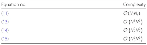
3.3 Complexity analysis of EKF

For the complexity analysis of the proposed joint chan-nel and PN estimation technique, we take the approach used by [36,37] and count the number of multiplications and additions used in each step of EKF algorithm. Table2

shows the complexity of each step of EKF algorithm using O−notation. The corresponding complexity calculations for this table can be found in Appendix5.

Table 2Complexity of each step of EKF algorithm

Equation no. Complexity

(11) O(NtNr)

(13) ON2

tN3r

(14) ON2_tN2

r

(15) ON3_tN3_r

Remark 3 According to Table (2), the EKF has a poly-nomial complexity as a function of number of transmit Nt and receive Nrantennas. We can justify the increased com-plexity as follows. In[20], the authors propose an algorithm for channel estimation with linear complexity. However, the algorithm in[20]assumes a constant PN for a block of data. This could be an acceptable scenario in microwave communication but does not suit mmWave communica-tion. Hence, the increased complexity of the proposed algo-rithm is justified because of fast variation of PN, i.e., PN variation over symbol time.

4 Simulation results

In this section, we present simulation results for MIMO FD systems at 60 GHz frequency, which corresponds to mmWave frequency band [3]. For each simulation run, we assume a communication packet is 40 symbol long, i.e.,

N = 40. This communication packet is transmitted after the training packet, which is 2Ntsymbols long, and is used for estimating the constant channels for EKF initialization as described in Section3.1. We then use 10,000 simulation runs to obtain the desired simulation results.

Moreover, we use the assumptions presented in Section2to generate the random noise and PN. As sum-marized in [38], there are many mmWave channel models available for mmWave systems. In this work, similar to a large number of existing works in [24, 29,39–41], we adopt a general Rician model. Note that the proposed estimator is independent of the adopted model. A per-formance comparison of the different mmWave channel models is outside the scope of this work.

We generate the random SI and communication channel (HSI/COM) using Rician distribution as follows:

HSI/COM =

&

K

K+1HLoS+

&

1

K+1HNLoS, (20) where K is the Rician distributionK-factor;HLoS is the

LoS component of the channel, and is generated assum-ing uniform distribution for angle of arrival, usassum-ing the approach presented in [24]; HNLoS is the NLoS

compo-nent of the channel; and for both SI and communication channel is generated assuming Rayleigh fading. Further-more, for both the SI and communication channel, we set theK-factor to 2 dB.

We note that the SI and communication channels have different power intensities, i.e., EHSIH†_SI

= EHCOMH†_COM

. Assuming that the LoS power of the residual SI (SI signal after the passive and analog cancela-tion) is the same as the LoS power of the communication signal, the signal to interference ratio (SIR) is given by:

SIR= σ

2 COM

σ2 SI

whereσ_COM2 andσ_SI2 are the variances of NLoS compo-nents of the communication and SI channels, respectively.

In addition, SNR is defined as

SNR E[Es]

σ2 , (22)

whereEsis the symbol energy,E[Es]=1, andσ2is the noise variance.

Finally, we use the MSE for the state vector at timeN=

40. This MSE is given by rewriting (18) in terms of the Euclidean norm of a vector, i.e.,|| · ||2,

E''''''β(N)−βˆ(N)'''''' 2

. (23)

In what follows, we first present the MSE results for different FD MIMO communication systems. We then investigate the residual SI power after digital cancelation and the bit error rate (BER) performance of these systems with the proposed PN estimation technique.

4.1 MSE performance

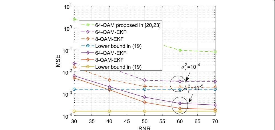
In this section, we investigate the MSE performance of the proposed PN estimation technique for a 2×2 FD MIMO system and assume that SIR=0 dB, i.e., the SI signal is as strong as the desired communication signal.

Figure 3 shows the MSE performance of the pro-posed system against the derived theoretical bound in Section 3.2 for different quadrature amplitude modula-tions (QAM) and different PN variances. Firstly, as dis-cussed in Remark 2, with increasing PN variance, the estimation performance degrades. Secondly, it can be observed from this figure that lower order modulations

have better performance compared to the higher order modulations. This is because as shown in Section3.1, the EKF algorithms require to detect the transmitted symbols. Hence, the MSE of EKF is affected by the detection error. Finally, Fig.3shows that at high SNRs, the MSE perfor-mance of the proposed estimator approaches the lower bound.

In Fig.3, we also plot the MSE result of the state-of-the-art pilot-based phase noise estimator in [20,23] for microwave frequency. As expected, this estimator does not perform well compared to our proposed estimator. This is because it assumes that the PN variations are small, which is not applicable for the case for mmWave fre-quency. Note that we only show the MSE result of the estimator in [20,23] for 64−QAM modulation since the MSE performance is invariant with respect to the modula-tion order (the estimator uses pilots and does not require detection).

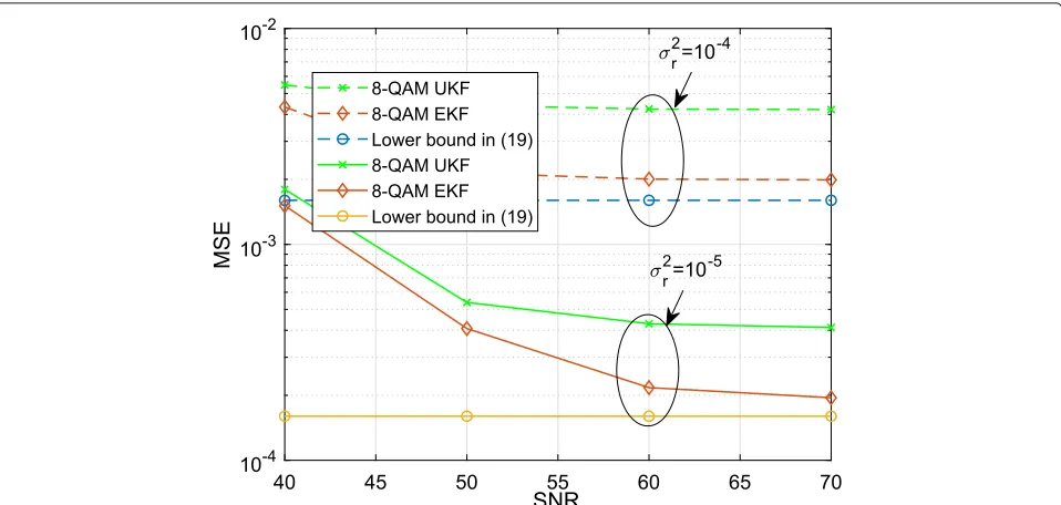
4.2 Comparison with unscented Kalman filter

We compare the performance of the proposed EKF esti-mator with unscented Kalman filter (UKF). UKF pro-vides an alternative for linearizing the observations. The detailed implementation of the UKF is provided in Appendix5. Figure4shows the performance of the EKF and UKF estimators for 8−QAM modulation, SIR=0 dB, and different PN variances. We can see that the MSE per-formance of the proposed EKF estimator is better than the UKF estimator. This is because (i) UKF estimator works with the sigma point approximation of the mean of the state process, while EKF tracks the PN based on the true

Fig. 3MSE performance for PN variancesσ2

Fig. 4MSE performance of the UKF and proposed EKF for PN variancesσ2

r =σt2=σSI2=10−4, 10−5and 8–QAM modulation for a 2×2 FD MIMO system with SIR=0 dB

mean of the linear state vector; (ii) while the MSE per-formances of both EKF and UKF are degraded because of the detection error, this error affects UKF algorithm more than EKF. This is because the sigma points calculation are affected more by the error due to the symbol detec-tion (Secdetec-tion3.1); and (iii) UKF is inherently more suitable for the systems which experience high nonlinearities, i.e., both the state and process models are nonlinear and noise is nonlinear too. In our case, only the process model in (7) is nonlinear.

4.3 Residual SI power

In this section, we numerically investigate the remaining SI power after digital cancelation for a 2×2 MIMO FD system with 64−QAM modulation, assuming the PN vari-ance for all the oscillators is 10−4. This residual power is given by

PSI=''''''

HSI(n)− ¯HSI(n)xSI(n)''_'''_'

2, (24)

where||·||2is the Euclidean norm of a vector, andH¯SI(n)is

an estimate of the SI channel using the proposed EKF esti-mator. Figure5shows the residual SI power for different SIR values, where a SIR value of 0 dB indicates that passive and analog cancelation stages have managed to reduce the SI power to the same level as the desired signal power.

The numerical result of Fig. 5 shows that the perfor-mance of digital canceler depends on the residual SI power after passive and analog cancelation stages. As the residual SI power after passive and analog cancelation decreases,

so does the residual SI power after the digital cancela-tion. The results show that the residual SI power can be reduced to −25 and −40 dB for SIR of 0 and 15 dB, respectively. This is important as it shows the effec-tiveness of digital SI cancelation after passive and analog cancelation.

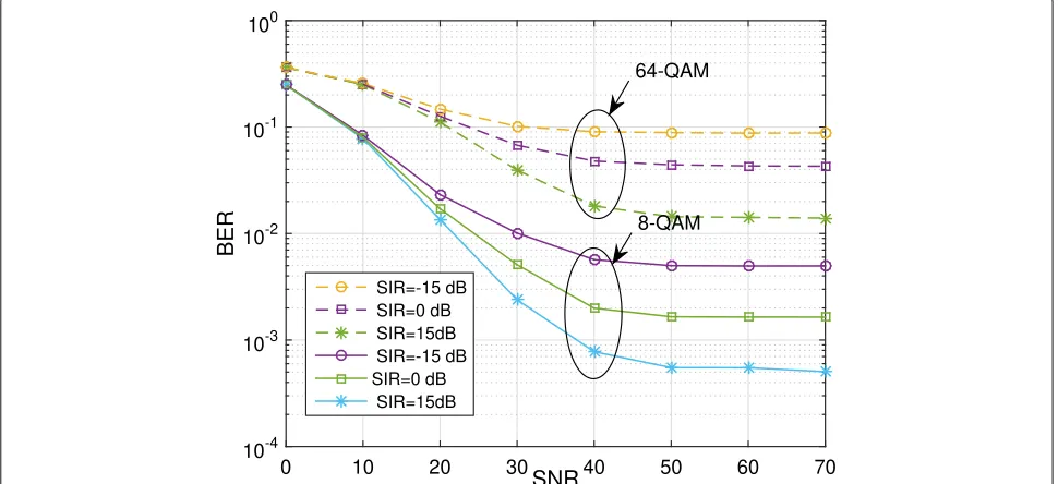
4.4 BER performance

Finally, in this section, we present the BER results of a 2 × 2 FD MIMO system with different QAM modula-tions, assuming that PN variance for all oscillators is 10−4. Figure6shows the BER performance of the system for dif-ferent values of SIR. The results are consistent with the results of the residual SI power in Fig. 5, i.e., the higher the SIR, the better the BER results. Furthermore, 8−QAM system performs better than the 64−QAM system, which is consistent with the results of Fig.6.

5 Conclusion

In this paper, we considered a MIMO FD system for mmWave communication and proposed a joint channel and PN estimation algorithm1_{. We also derived a lower}

Fig. 5The residual SI powerPSIafter digital cancelation

Endnote

1_{Indeed, the main focus of this work is to correctly}

estimate the channel and PN for effective SI cancela-tion. In case of inter-node interference [45], the proposed estimator would need to be modified. However, in the special case, if the inter-node interference can be treated as Gaussian, then the system model given by (1) can

capture the effect of the inter-node interference by includ-ing an additional Gaussian noise term due to inter-node interference.

A lower bound of the estimation error

In this section, we derive the lower bound of the estimation error. We start the proof by expanding

E#β(n)−βˆ(n) β(n)−βˆ(n)

Consequently, we can rewrite (25) as follows:

E#β(n)−βˆ(n) β(n)−βˆ(n)T

Furthermore, the properties oftraceallows us to write

trace and (18), we can establish the proof of the proposition.

B Complexity analysis of EKF

In this section, we provide the complexity analysis of the EKF algorithm by counting the number of multiplica-tions and addimultiplica-tions. However, before we proceed, it can easily be shown that every entry of product of a K ×L

matrix by aL×Mmatrix requiresLmultiplications and

L−1 additions, and hence, the whole matrix requiresKML

multiplications and KM(L− 1) additions, where KM is the size of the resulting matrix. Furthermore, it is known that matrix inversion has the same complexity in terms of additions and multiplication as the matrix multiplication, up to a multiplicative constantγ [42]. We can now pro-ceed with calculating the complexity of EKF algorithm in (30) to (32).

C Unscented Kalman filter (UKF)

the state vector (8), has a linear state process and addi-tive noise. This allows for the use of non-augmented state vectors for UKF [44]. For the state vectorβ(n)in (8), the given by (9). Subsequently, the mean of the sigma points, which is used as an approximate to the true mean of the probability distribution of states, is given by

¯

Similarly, the covariance of the state vector based on the sigma points approximation is given by

¯

Moreover, the sigma points for the observations, and the corresponding approximate mean of probability distribu-tion of observadistribu-tions are given by

Y(n|n−1)= ¯H(n)ejB(i,n|n−1), (38a) models are approximated by the sigma points using (33a)– (33c), and (38a), respectively, the updated meanβˆ(n)and variancePˆncan be calculated as follows:

ˆ

β(n)= ¯β(n)+K(y(n)− ¯y(n)), (39) ˆ

Pn= ¯Pn−KPy,yKT, (40)

Algorithm 1UKF for joint channel and PN estimation

1: Initialize:

5: Calculate the covariance matrix of the state vector using (37).

6: Calculate the sigma points for observations using (38a).

7: Calculate the mean of observation using (38b).

8: Update the meanβˆ(n)using (39).

Algorithm 1 summarizes the UKF joint channel and PN estimation algorithm.

Acknowledgements

The authors would like to thank Professor Taneli Rihhonen for his insightful comments on this work.

Funding

The work of Abbas Koohian was supported by an Australian Government Research Training Program (RTP) Scholarship. The work of Hani Mehrpouyan was partially funded by the NSF ERAS grant award number 1642865.

Authors’ contributions

All authors contributed equally to this work. The final manuscript has been read and approved by all authors for submission.

Competing interests

The authors declare that they have no competing interests.

Publisher’s Note

Springer Nature remains neutral with regard to jurisdictional claims in published maps and institutional affiliations.

Author details

1_{Research School of Electrical, Energy, and Materials Engineering, Australian} National University, Canberra, Australia.2_{Department of Electrical and} Computer Engineering, Boise State University, Boise, ID, USA.3_{Department of} Electrical Engineering, King Fahd University of Petroleum and Minerals, Dhahran, Saudi Arabia.

References

1. S. A. Busari, K. M. S. Huq, S. Mumtaz, L. Dai, J. Rodriguez, Millimeter-wave massive MIMO communication for future wireless systems: a survey. IEEE Commun. Surveys Tuts.20(2), 836–869 (2018)

2. R. W. Heath, N. Gonzalez-Prelcic, S. Rangan, W. Roh, A. M. Sayeed, An overview of signal processing techniques for millimeter wave MIMO systems. IEEE J. Sel. Topics Signal Process.10(3), 436–453 (2016) 3. T. S. Rappaport, S. Sun, R. Mayzus, H. Zhao, Y. Azar, K. Wang, G. N. Wong,

J. K. Schulz, M. Samimi, F. Gutierrez, Millimeter wave mobile

communications for 5G cellular: it will work! IEEE Access.1, 335–349 (2013) 4. S. Rajagopal, S. Abu-Surra, J. Zhang, inProc. IEEE SPAWC. Spectral mask

filling for PAPR reduction in large bandwidth mmWave systems, (2015), pp. 131–135

5. S. Buzzi, C. D’Andrea, T. Foggi, A. Ugolini, G. Colavolpe, Single-carrier modulation versus OFDM for millimeter-wave wireless MIMO. IEEE Trans. Commun.66(3), 1335–1348 (2018)

6. M. Duarte, C. Dick, A. Sabharwal, Experiment-driven characterization of full-duplex wireless systems. IEEE Trans. Wireless Commun.11(12), 4296–4307 (2012)

7. Z. Zhang, X. Chai, K. Long, A. V. Vasilakos, L. Hanzo, Full duplex techniques for 5G networks: self-interference cancellation, protocol design, and relay selection. IEEE Commun. Mag.53(5), 128–137 (2015)

8. H. Mehrpouyan, M. R. Khanzadi, M. Matthaiou, A. M. Sayeed, R. Schober, Y. Hua, Improving bandwidth efficiency in E-band communication systems. IEEE Commun. Mag.52(3), 121–128 (2014)

9. V. Syrjala, M. Valkama, L. Anttila, T. Riihonen, D. Korpi, Analysis of oscillator phase-noise effects on self-interference cancellation in full-duplex OFDM radio transceivers. IEEE Trans. Wirel. Commun.13(6), 2977–2990 (2014) 10. S. Hong, J. Brand, J. Choi, M. Jain, J. Mehlman, S. Katti, P. Levis, Applications

of self-interference cancellation in 5G and beyond. IEEE Commun. Mag. 52(2), 114–121 (2014)

11. A. Koohian, H. Mehrpouyan, M. Ahmadian, M. Azarbad, inProc. IEEE ICC. Bandwidth efficient channel estimation for full duplex communication systems, (2015), pp. 4710–4714

12. M. Duarte, A. Sabharwal, inProc. Asilomar Conf. on Signals, Syst. and Computers. Full-duplex wireless communications using off-the-shelf radios: feasibility and first results, (2010), pp. 1558–1562

13. M. Duarte, A. Sabharwal, V. Aggarwal, R. Jana, K. K. Ramakrishnan, C. W. Rice, N. K. Shankaranarayanan, Design and characterization of a full-duplex multiantenna system for WiFi networks. IEEE Trans. Veh. Technol.63(3), 1160–1177 (2014)

14. E. Everett, A. Sahai, A. Sabharwal, Passive self-interference suppression for full-duplex infrastructure nodes. IEEE Trans. Wirel. Commun.13(2), 680–694 (2014)

15. A. A. Nasir, S. Durrani, H. Mehrpouyan, S. D. Blostein, R. A. Kennedy, Timing and carrier synchronization in wireless communication systems: a survey and classification of research in the last 5 years. EURASIP J. Wirel. Commun. Netw.180(1) (2016). Available: https://doi.org/10.1186/s13638-016-0670-9

16. E. Ahmed, A. M. Eltawil, On phase noise suppression in full-duplex systems. IEEE Trans. Wirel. Commun.14(3), 1237–1251 (2015)

17. B. Lee, J. B. Lim, C. Lim, B. Kim, J. Y. Seol, inProc. IEEE Globecom Workshops. Reflected self-interference channel measurement for mmWave beamformed full-duplex system, (2015), pp. 1–6

18. A. Demir, T. Haque, E. Bala, P. Cabrol, inProc. WAMICON. Exploring the possibility of full-duplex operations in mmWave 5G systems, (2016), pp. 1–5

19. T. A. Thomas, M. Cudak, T. Kovarik, inProc. IEEE ICC. Blind phase noise mitigation for a 72 GHz millimeter wave system, (2015), pp. 1352–1357 20. A. Masmoudi, T. Le-Ngoc, A maximum-likelihood channel estimator for

self-interference cancelation in full-duplex systems. IEEE Trans. Veh. Technol.65(7), 5122–5132 (2016)

21. A. Masmoudi, T. Le-Ngoc, Channel estimation and self-interference cancelation in full-duplex communication systems. IEEE Trans. Veh. Technol.66(1), 321–334 (2017)

22. X. Xiong, X. Wang, T. Riihonen, X. You, Channel estimation for full-duplex relay systems with large-scale antenna arrays. IEEE Trans. Wireless Commun.15(10), 6925–6938 (2016)

23. R. Li, A. Masmoudi, T. Le-Ngoc, Self-interference cancellation with nonlinearity and phase-noise suppression in full-duplex systems. IEEE Trans. Veh. Technol.67(3), 2118–2129 (2018)

24. H. Mehrpouyan, A. A. Nasir, S. D. Blostein, T. Eriksson, G. K. Karagiannidis, T. Svensson, Joint estimation of channel and oscillator phase noise in MIMO systems. IEEE Trans. Signal Process.60(9), 4790–4807 (2012)

25. D. Korpi, L. Anttila, V. Syrjala, M. Valkama, Widely linear digital

self-interference cancellation in direct-conversion full-duplex transceiver. IEEE J. Sel. Areas Commun.32(9), 1674–1687 (2014)

26. D. Korpi, T. Riihonen, V. Syrjala, L. Anttila, M. Valkama, R. Wichman, Full-duplex transceiver system calculations: analysis of ADC and linearity challenges. IEEE Trans. Wirel. Commun.13(7), 3821–3836 (2014) 27. L. Samara, M. Mokhtar, O. Ozdemir, R. Hamila, T. Khattab, Residual

self-interference analysis for full-duplex OFDM transceivers under phase noise and I/Q imbalance. IEEE Commun. Lett.21(2), 314–317 (2017) 28. E. Ahmed, A. M. Eltawil, A. Sabharwal, Rate gain region and design

tradeoffs for full-duplex wireless communications. IEEE Trans. Wirel. Commun.12(7), 3556–3565 (2013)

29. A. A. Nasir, H. Mehrpouyan, R. Schober, Y. Hua, Phase noise in MIMO systems: Bayesian Cramer Rao bounds and soft-input estimation. IEEE Trans. Signal Process.61(10), 2675–2692 (2013)

30. K. I. Pedersen, G. Berardinelli, F. Frederiksen, P. Mogensen, A. Szufarska, A flexible 5G frame structure design for frequency-division duplex cases. IEEE Commun. Mag.54(3), 53–59 (2016)

31. S. Dutta, M. Mezzavilla, R. Ford, M. Zhang, S. Rangan, M. Zorzi, Frame structure design and analysis for millimeter wave cellular systems. IEEE Trans. Wirel. Commun.16(3), 1508–1522 (2017)

32. C. Gustafson, K. Haneda, S. Wyne, F. Tufvesson, On mm-wave multipath clustering and channel modeling. IEEE Trans. Antennas Propag.62(3), 1445–1455 (2014)

33. D. Kim, H. Ju, S. Park, D. Hong, Effects of channel estimation error on full-duplex two-way networks. IEEE Trans. Veh. Technol.62(9), 4666–4672 (2013)

34. M. R. Khanzadi, R. Krishnan, D. Kuylenstierna, T. Eriksson, inProc. IEEE Globecom Workshops. Oscillator phase noise and small-scale channel fading in higher frequency bands, (2014), pp. 410–415

35. S. M. Kay,Fundamentals of Statistical Signal Processing: Estimation Theory. (Prentice-Hall, Inc., Upper Saddle River, 1993)

36. A. A. Nasir, H. Mehrpouyan, S. D. Blostein, S. Durrani, R. A. Kennedy, Timing and carrier synchronization with channel estimation in multi-relay cooperative networks. IEEE Trans. Signal Process.60(2), 793–811 (2012) 37. A. Koohian, H. Mehrpouyan, A. A. Nasir, S. Durrani, S. D. Blostein,

Superimposed signaling inspired channel estimation in full-duplex systems. EURASIP J. Adv. Signal Process.8(2018). Available:https://doi. org/10.1186/s13634-018-0529-9

38. I. A. Hemadeh, K. Satyanarayana, M. El-Hajjar, L. Hanzo, Millimeter-wave communications: physical channel models, design considerations, antenna constructions, and link-budget. IEEE Commun. Surveys Tuts. 20(2), 870–913 (2018)

39. A. G. Siamarou, Digital transmission over millimeter-wave radio channels: a review [wireless corner]. IEEE Antennas Propag. Mag.51(6), 196–203 (2009)

40. J. Zhang, L. Dai, X. Zhang, E. Bjornson, Z. Wang, Achievable rate of rician large-scale MIMO channels with transceiver hardware impairments. IEEE Trans. Veh. Technol.65(10), 8800–8806 (2016)

41. T. S. Rappaport, G. R. MacCartney, S. Sun, H. Yan, S. Deng, Small-scale, local area, and transitional millimeter wave propagation for 5G

communications. IEEE Trans. Antennas Propag.65(12), 6474–6490 (2017) 42. S. Arora, B. Barak,Computational Complexity: A Modern Approach, 1st edn.

(Cambridge University Press, New York, 2009)

43. E. A. Wan, R. V. D. Merwe, inProc. IEEE Adaptive Systems for Signal Processing, Communications, and Control Symposium. The unscented Kalman filter for nonlinear estimation, (2000), pp. 153–158

44. Y. Wu, D. Hu, M. Wu, X. Hu, Unscented Kalman filtering for additive noise case: augmented versus nonaugmented. IEEE Signal Process. Lett.12(5), 357–360 (2005)