Comparing Poverty and Deprivation Dynamics: Issues of Reliability and Validity EPAG Working Paper 53, 2005

1

Comparing Poverty and Deprivation

Dynamics: Issues of Reliability and Validity

Christopher T. Whelan and Bertrand Maître

The European Panel Analysis Group (EPAG) is a consortium of European social and

economic researchers who have been collaborating since 1990 in the development

and analysis of household panel surveys in the European Union. Most recently it has

been engaged in the study of flexible labour and its impact on earnings and poverty

under a Eurostat contract, and a programme of research on social exclusion as part

of the EU's Targeted Socio-Economic Research programme. The group has set up

new comparative datasets based on five-year sequences of the British, German and

Dutch national household panels, and is analysing the early data from the European

Community Household Panel (ECHP). Most of the research to date has been in the

fields of family formation, employment, household income and 'deprivation'.

The group was awarded a grant under the EU's Fifth Framework Programme

"Improving Human Potential and the Socio-Economic Knowledge Base" to undertake

studies of the processes of change in the domains of family structure, employment,

household income and living standards. This project - "The Dynamics of Social

Change in Europe"- began in March 2000, and is based primarily on the quantitative

analysis of ECHP data.

The members of EPAG are:

Institute for Social and Economic

Research

(ISER)

University of Essex

, United Kingdom

(led by Richard Berthoud and

Jonathan Gershuny)

Economic and Social Research

Institute

(ESRI)

Dublin, Ireland

(led by Brian Nolan and

Chris Whelan)

German Institute for Economic

Research

(DIW)

Berlin, Germany

(led by Gert G. Wagner and

C. Katharina Spiess)

Tilburg Institute for Social Security

Research (TISSER)

Catholic University of Brabant

,

Tilburg, Netherlands

(led by Ruud Muffels)

Centre for Labour Market and

Social Research (CLS

University of Aarhus

, Denmark

(led by Peder Pedersen and

Nina Smith)

Department of Sociology and Social

Research (DSSR)

University of Milano-Bicocca,

Italy

(led by Antonio Schizzerotto)

Acknowledgement:

Data from the European Community Household Panel Survey

1994-8 are used with the permission of Eurostat, who bear no responsibility for the

analysis or interpretations presented here. We would like to thank Richard Breen and

Pasi Moisio for comments on a earlier version of this paper. All remaining errors are

the responsibility of the authors. We would like to thank Pasi Moisio for making a

number of programmes and routines available to us and for helpful advice on a

range of issues.

Readers wishing to cite this document are asked to use the following form of words:

Whelan, Christopher, T., Maitre, Bertrand. (February 2005) ‘Comparing

Poverty and Deprivation Dynamics: Issues of Reliability and Validity’,

EPAG

number 53. Colchester: University of Essex

For an on-line version of this working paper and others in the series, please visit the Institute’s website at: http://www.iser.essex.ac.uk/epag/pubs/

 February 2005

ABSTRACT

In this paper we seek to establish if earlier findings relating to the relationship between income poverty persistence and deprivation persistence could be due to a failure to take measurement error into account. In order to address this question, we apply a model of dynamics incorporating structural and error components. Our analysis shows a general similarity between latent poverty and deprivation dynamics. In both cases all unsystematic error is captured as change and we substantially overestimate mobility. Distinguishing between different types of reliability we find that by far the largest component of error is associated with overestimation of the probability of exiting from poverty or deprivation. We observe a striking similarity across dimensions at both observed and latent levels. In both cases levels of poverty and deprivation persistence are higher at the latent level. However, there is no evidence that earlier results relating to the differences in the determinants of poverty and deprivation persistence are a consequence of differential patterns of reliability. Taking measurement error into account seems more likely to accentuate rather than diminish the contrasts highlighted by earlier research. Since longitudinal differences relating to poverty and deprivation cannot be accounted for by measurement error, it seems that we must accept that we are confronted with issues relating to validity rather than reliability. Even where we measure these dimensions over reasonable periods of time and allow for measurement error, they continue to tap relatively distinct phenomenon. Thus, if measures of persistent poverty are to constitute an important component of EU social indicators, a strong case can be made for including parallel measures of deprivation persistence and continuing to explore the relationship between them.

Comparing Poverty and Deprivation Dynamics: Issues of Reliability and Validity

In recent years the availability of the European Community Household Panel (ECHP) has made it

possible to undertake a comparative analysis of the relationship between income poverty and

deprivation measures at both cross-sectional and longitudinal levels. Interest in exploring this

relationship has been stimulated, as Perry (2002) notes in a recent review of the literature, by the

observation that there is a significant mismatch between poverty measured indirectly using an income

approach and direct measures focusing on life-style deprivation. As has been recognised for sometime,

this presents a challenge to the use of relative income poverty lines when identifying those excluded

from a minimal acceptable standard of living through a lack of resources.1 _{The issue raised here is one}

of validity i.e. whether it is reasonable to interpret relative income measures as adequately capturing

such exclusion. Our starting point in this paper is the finding by Whelan et al (2004) that even where we

employ longitudinal measures income poverty and deprivation appear to be tapping different

phenomena. Our objective is to establish the extent to which this conclusion may be affected by the fact

these dimensions are differentially affected by measurement error.

As Moisio (2004: 55) notes it has become a good deal less common to think of validity in purely

statistical terms and attention is most frequently focused on construct validity and the need to provide a

conceptual justification of the measure employed locating it in relation to alternative measures and

conceptual frameworks. In the case of income poverty measurement such efforts have led to increased

focus on both multi-dimensional and longitudinal measurement. In this paper we wish to consider the

possibility that by paying appropriate attention to the longitudinal aspect we may avoid the need for

multidimensional measurement suggested by the observed mismatch between income poverty and

deprivation apparent at the cross-sectional level. A particularly strong version of the hypothesis that the

key to resolving these issues lies in using longitudinal measures is that of Gordon (2002:15) who

suggests that different measures tap the same dynamic process but in its different phases. Without

going this

far we might expect that by measuring poverty and deprivation over time we could make significant

progress in reducing the mismatch associated with point in time measures. Panel research has shown

that movements into and out of poverty are a great deal more frequent than had been supposed and

1

that a far greater proportion of the population experience poverty at some point than revealed by

cross-sectional studies (Layte & Whelan 2003). By extending our measure of income poverty over time, we

might hope to get a better measure of permanent income or command of resources. Our expectation

would then be that such a measure would be more strongly related to deprivation and would contribute

to a reduction in the income poverty-deprivation mismatch. Implicit in this approach is the assumption

that deprivation measures are more stable than income measures and thus that current level of

deprivation is a significantly better indicator of persistent deprivation than current income is of its

longitudinal counterpart. Given this, the mismatch problem, evident at the cross-sectional level, would

be largely resolved by taking poverty experience over time into account.

A recent analysis by Whelan et al (2002) sought to test these hypotheses using the first five waves of

the ECHP. Their findings turned out to be remarkably stable across the nine countries included in their

analysis. In each case a measure of extent of exposure to poverty over the five-year spell offered

significant advantages over its cross-sectional counterpart. An income poverty profile schema that

differentiated respondents in terms of their degree of exposure was shown to be systematically related

to both cross-sectional and longitudinal deprivation. However, contrary to expectations, the level of

mismatch at the longitudinal level was no less than for point-in-time measures.

Thus even where we are in a position to observe both income poverty and life-style deprivation over a

reasonable period of time the evidence points to the conclusion that, while there is a substantial

correlation between these dimensions, they are to a significant extent tapping different phenomena.

Thus, if poverty continues to be defined in terms of “exclusion from a minimally acceptable standard of

living through a lack of resources” it is necessary to conclude that even longitudinal measures of

income poverty cannot be taken on their own as providing valid measures of the underlying construct

and it remains necessary to take into account direct measures of deprivation. However, one factor that

has not been taken into account in earlier analyses is the role of measurement error. This is not

unusual and indeed Breen and Mosio (forthcoming) could find only one effort prior to their own by

Rendtel et al (1998) that developed a model to distinguish between true poverty mobility and

measurement error. As they note, conclusions about poverty dynamics drawn on the basis of observed

data implicitly assume a saturated structural model and a measurement model that assumes exact

correspondence between observed poverty and true poverty. Studies of this kind based on the ECHP

have shown generally show high levels of mobility into and out of poverty with a much larger proportion

of the population experiencing poverty at some point during the period of observation than suggested

part of the population (Layte and Whelan, 2003, Whelan et al 2004). As Breen and Moisio (forthcoming)

note, these two aspects of poverty dynamics seem to surface in one form or other in most studies of the

phenomenon. 2

While there is a remarkable consistency in such findings, recent studies that have taken measurement

error in account produce a strikingly different picture. As Moisio (2004:58) notes, measurement error in

relation to income poverty can arise for a variety of reasons. The respondent may report erroneous

information relating to either income components or household composition. Surveys request income

over a fixed period such as the previous year and respondents may have different perceptions of time

in relation to income. The meaning of ‘household’ may be misunderstood. Finally there may be sources

of income that the respondent does not wish to reveal. With the measures of life-style deprivation we

employ respondents are in most case asked to indicate not only the presence or absence of an item but

in the case of absence whether this arises because of inability to afford the item. There are thus two

distinct sources of error. Moisio (2004:59) notes that, while with cross-sectional measures we may

reasonably assume that measurement errors cancel out each other, so that our estimates are unbiased

if random errors are uncorrelated, this convenient attribute does not apply with repeated measures.

Rendtel et al (1998) using a latent Markov chain model reached the striking conclusion that almost half

the observed poverty mobility in the German Socio-Economic Panel could be accounted for by

measurement error. Basic et al (2004) extended such analysis by applying such models to a

comparison of the first wave of the Finnish ECHP survey and corresponding administrative data and

concluded that over-estimation of poverty transitions as a consequence of measurement error was a

substantially more serious problem than errors in estimation associated with selective attrition.

Breen and Moisio (forthcoming) and Moisio (2004) apply a range of models of graduated complexity to

income poverty dynamics in ten countries using four waves of the ECHP. These models range from a

simple Markov model to a time-heterogeneous mover-stayer model that allows error in the

measurement of the movers’ states. The simple Markov chain model assumes that the state occupied

at time t depends only on the state occupied at time t-1. The most parsimonious version restricts the

two-way transition matrices to be stable across time while an alternative version allows for

heterogeneity. Such models, which assume a homogeneous population, rarely provide a satisfactory fit.

A mixed Markov model allows for more than one chain. The best known of such models is a

2

stayer model where the transition probabilities in the second chain relating to the stayers are assumed

to be either 1.00 or 0.0. The model thus assumes two underlying groups - one who are stable between

successive years and another involving individuals who move in and out of poverty according to a

simple Markov change process. This model takes no account of measurement error.

Such error can be taken into account by combining latent class and Markov chain modelling. Latent

structure models were developed by Lazarsfeld and Henry (1968).as measurement models that relate,

in a probabilistic, fashion, a discrete or continuous variable to the discrete scores or categories of

manifest variables. Van de Pol and De Leeuw (186) used such models to estimate measurement errors

in repeated nominal variables and provide a account of the location of measurement error.

The final model applied by Breen and Moisio (forthcoming), which provides the most satisfactory

account of income poverty dynamics across the ten countries included in their analysis, is a latent

mover-stayer model in which the movers’ chain is allowed to be heterogeneous over time.3 _Applying

this model they confirm the earlier result of Rendtel et al (1998, 2004) that mobility in income poverty

dynamics is overestimated by between 25 and 50 per cent if measurement error is ignored. In this

paper we wish to pursue the implications of these striking findings for earlier work concerning the

relationship between income poverty persistence and deprivation persistence. This work has shown

that these different forms of persistence display both distinct patterns of socio-economic variation and

highly variable consequences for outcomes such as subjective economic strain (Whelan et al 2003,

2004). These results suggest that these measure are tapping somewhat different underlying

dimensions. If, however, it were the case that deprivation persistence was measured with much greater

accuracy than was the case for income persistence then a significant part of the observed difference

might derive from differential reliability.

In the analysis that follows we will seek to explore these issues by applying the heterogeneous latent

mover-stayer model to both income poverty and deprivation dynamics for the range of countries for

which such information is contained in the User Data Base (UDB) of the ECHP.4 _{Moisio (2004) has}

applied this model and others to a housing deprivation index in the ECHP and found support for the

existence of a common pattern of fluidity at the latent but not at the observed level. However, in the

3

For an account of the full range of models applied by Breen and Moisio (fortcoming) and the corresponding LEM syntax (Vermunt, 1997) see Moisio (2004).

4

earlier analysis of Whelan et al (2003, 2004) housing items were deliberately excluded from the

deprivation index employed. Such items have been found to form a quite distinct cluster to those

included in the Current Life Style Deprivation (CLSD) index employed by Whelan et al. and to have

significantly weaker correlations with income.5 _{Given the role of life-cycle variables and the influence of}

factors such as the balance of private sector versus public sector provision, the weak association of

housing deprivation with income is not surprising and we therefore argue that the mismatch between

income and this form of deprivation does not constitute the same kind of problem with regard to

construct validity as that involving measures such the CLSD indicator that we propose to employ in our

subsequent analysis.6

Data and variables

The results presented in this paper are based on the ECHP User Data Base (UDB) containing data from

waves one to five (1994 to 1998) as released for public use by Eurostat.7 _{The income measure employed}

is total annual disposable household income, including transfers and after deduction of income tax and

social security contributions, with the household taken as the income recipient unit. In using total annual

income of the previous year, as we do in this paper, one concern one might have is about the possible

discrepancy between the time (t-1) the income refers to and the time of the interview (t). One solution to

this problem could be to match retrospectively the total annual income from the following wave at t +1

with the current wave (t) and to repeat this operation for the successive waves.8 _{However in this case}

one is also confronted to the problem that some household characteristics might have changed

between t and t+1, so the income taken from the following wave at t +1 might not necessarily coincide

with the same household characteristics at t time as it does at t +1. In addition one must jettison the

income data from the first wave. For this reason in this paper we prefer to use the total annual

household income reported within each wave and to use it with the current household characteristics

available in the same wave as given by Eurostat.

5

For discussions concerning the dimensionality of deprivation sees Dewilde, 2004, Perez-Mayo, 2003 and (Whelan, Layte, Maître, & Nolan 2001).

6

The distinctive character of housing deprivation is also confirmed by Moisio’s (2004:114) analysis where observed exit rates are remarkably high.

8 For a discussion of the quality of the ECHP data see Wirz and Meyer (2002).

8

We employ the “modified OECD” equivalence scale where the first adult in a household is given the value

1, each additional adult is given a value of 0.5 and each child a value of 0.3.9 _{The equivalised income of the}

household is attributed to each member, assuming a common living standard within the household.

While household income is used as the income concept, following standard procedures, the individual is

chosen as the unit of analysis.10 _{The individual is preferred to the household because the latter is not a}

stable entity over time since family composition often changes fundamentally over the years for various

reasons, such as birth and death, leaving home, divorce or separation and marriage and remarriage. In our

analysis of dynamics we use a balanced panel of ‘survivors’ who remained in the sample from 1994 to

1998 and use the ‘base weight’ as a longitudinal weight for this group as specified by Eurostat.11 _Although

the full ECHP UDB data file includes data for fifteen countries the data required for our analysis is available

for only nine countries. For these nine countries the total number of individual respondents in the first wave

was with 139,358 with 95,213 being available for analysis across the five waves from 1994-1998. 12

For the purposes of the analyses in this paper, we identified thirteen household items, which could

serve as indicators of the concept of life-style deprivation, understood as involving being denied the

opportunity to obtain goods, facilities and opportunities to participate in a manner generally identified as

appropriate in the relevant community. The items included in the scale are considered to cover a range

of what we term Current Life-Style Deprivations (CLSD). The format of the items varied, but in each

case we seek to use measures that can be taken to represent enforced absence of widely desired

items. 13

Respondents were asked about some items in the format employed by Mack & Lansley (1985): for

each household it was established if the item was possessed/availed of, and if not a follow-up question

asked if this was due to inability to afford the item. The following six items took this form:

• A car or van. • A colour TV.

10 The level of measured income inequality can vary depending on the choice of equivalence scale (see e.g. (Buhman et al. 1988)).

10

See (Muffels & Fouarge2003)

11

For a discussion of attrition in the ECHP see (Watson 2003)

12

For a discussion of the quality of the ECHP data see (Eurostat 1999b; Eurostat 1999a; Watson & Healy 1999) and (Wirz & Mejer 2002)

• A video recorder. • A micro wave. • A dishwasher. • A telephone.

In these cases we consider a household to be deprived only if absence is stated to be due to lack of

resources.

For some items the absence and affordability elements were incorporated in one question, as follows:

“There are some things many people cannot afford even if they would like them. Can I just check

whether your household can afford these if you want them”. The following six items were administered

in this fashion:

• Keeping your home adequately warm.

• Paying for a week’s annual holiday away from home. • Replacing any worn-out furniture.

• Buying new, rather than second hand clothes.

• Eating meat chicken or fish every second day, if you wanted to. • Having friends or family for a drink or meal at least once a month.

The final item relates to arrears; we consider a household as experiencing deprivation in terms of this

item if it was unable to pay scheduled mortgage payments, utility bills or hire purchase instalments

during the past twelve months. An index based on a simple addition of these thirteen items give a

reliability coefficient of 0.80.

We use a weighted version of this measure in which each individual item is weighted to the proportion

of households suffering an enforced lack of that item in each country. The weighted CLSD measure

makes it possible to identify for each country, and for each income poverty line, a corresponding

deprivation threshold where the proportions of persons in income poverty and in deprivation are the

same. For example if in the Netherlands 20% of persons are below the 70% income poverty line we

calculate a deprivation threshold identifying the 20th _{% of persons the most deprived on the weighted}

CLSD measure. This allows for the mismatch between poverty defined in income and deprivation terms

We have chosen to focus on the 70% median income line. Given that our analysis covers five years,

opting for a lower threshold would create difficulties arising from sparse observations in a number of

cells of the five-way transition table, particularly those involving persistent income poverty. Thus in

Breen and Moisio’s (forthcoming) analysis of the four waves of the ECHP in only one case did the

percentage falling below this line in all four years exceed ten per cent and in only three out of ten did it

exceed seven per cent. For five waves these rates will necessarily be lower. In most countries this

problem is even greater if we focus on deprivation.

Observed Income poverty and Deprivation Dynamics

Before proceeding to model poverty and deprivation dynamics we provide an account of the observed

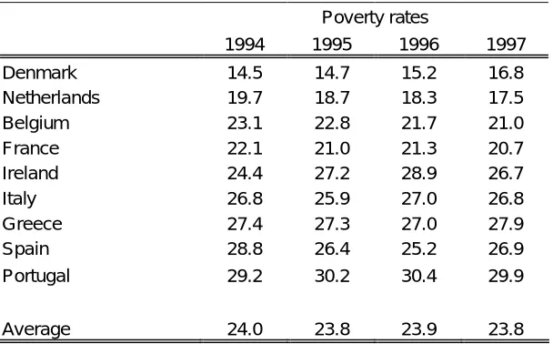
patterns. In Table 1 we set out the cross-sectional poverty rates for the balanced panel. We can see

that poverty dynamics during the first five waves took place in the context of relatively little variation in

the cross-sectional rates. In the first wave the rate varied from 14.5% in Denmark to 29.2% in Portugal.

Between the first and fifth waves the rate increase by 4% in Denmark and declined by 3% in Spain,

otherwise variation was extremely modest and obviously plays a modest role in structuring poverty

dynamics.

Table 1: Observed income poverty rates in each wave

Poverty rates

1994 1995 1996 1997

Denmark 14.5 14.7 15.2 16.8

Netherlands 19.7 18.7 18.3 17.5

Belgium 23.1 22.8 21.7 21.0

France 22.1 21.0 21.3 20.7

Ireland 24.4 27.2 28.9 26.7

Italy 26.8 25.9 27.0 26.8

Greece 27.4 27.3 27.0 27.9

Spain 28.8 26.4 25.2 26.9

Portugal 29.2 30.2 30.4 29.9

Average 24.0 23.8 23.9 23.8

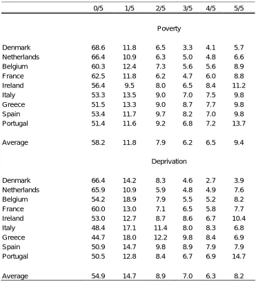
In Table 2 we show the percentage classified as poor N times out 5 for both income poverty and

deprivation. The proportion exposed to poverty at any point during the five years ranged from 31.4% in

Denmark to 48.6% in Portugal. As with earlier work there is a remarkable uniformity in the ratio of the

“ever-poor” figure to the poverty rate in the first wave. The observed values all lie in the narrow range

ranges from 5.7% in Denmark to 13.7% in Portugal. The “always poor” rate ranges between

approximately one-third and less than one half of the cross-sectional rates. The figures for deprivation

persistence are very similar to those for income poverty. Thus the percentage exposed to poverty on at

least one occasion ranges from 34% in the Netherlands to 47% in Ireland. The average difference

between the poverty and deprivation figures is of the order of three per cent. Similarly the proportion

experiencing poverty in all five years ranges from 3.9% in Denmark to 14.7% in Portugal, with average

difference between the poverty and deprivation figures being less than two per cent.

Table 2: Proportion classified as poor and deprived N times out of five

0/5 1/5 2/5 3/5 4/5 5/5

Poverty

Denmark 68.6 11.8 6.5 3.3 4.1 5.7

Netherlands 66.4 10.9 6.3 5.0 4.8 6.6

Belgium 60.3 12.4 7.3 5.6 5.6 8.9

France 62.5 11.8 6.2 4.7 6.0 8.8

Ireland 56.4 9.5 8.0 6.5 8.4 11.2

Italy 53.3 13.5 9.0 7.0 7.5 9.8

Greece 51.5 13.3 9.0 8.7 7.7 9.8

Spain 53.4 11.7 9.7 8.2 7.0 9.8

Portugal 51.4 11.6 9.2 6.8 7.2 13.7

Average 58.2 11.8 7.9 6.2 6.5 9.4

Deprivation

Denmark 66.4 14.2 8.3 4.6 2.7 3.9

Netherlands 65.9 10.9 5.9 4.8 4.9 7.6

Belgium 54.2 18.9 7.9 5.5 5.2 8.2

France 60.0 13.0 7.1 6.5 5.8 7.7

Ireland 53.0 12.7 8.7 8.6 6.7 10.4

Italy 48.4 17.1 11.4 8.0 8.3 6.8

Greece 44.7 18.0 12.2 9.8 8.4 6.9

Spain 50.9 14.7 9.8 8.9 7.9 7.9

Portugal 50.5 12.8 8.4 6.7 6.9 14.7

Average 54.9 14.7 8.9 7.0 6.3 8.2

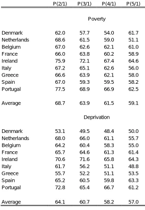
As in the case of the earlier analysis by Breen and Moisio (forthcoming), while poverty spells are

generally of short duration the risk of poverty recurring remains persistently high. From Table 3 we can

see that, given that one is income poor in wave one, the risk of poverty recurring declines very

by the fifth wave it was still as high as 0.59.14 _{So relatively modest overall risks of uninterrupted poverty}

go together with high levels of recurrence. The results for deprivation are remarkably similar with the

conditional risk of being above the deprivation threshold in the second wave being 0.64 with a modest

decline to 0.57 by wave five. Overall the observed poverty and deprivation mobility patterns, rather than

suggesting greater stability and persistence for the deprivation dimension reveal remarkably similar

patterns for both variables. In the section that follows our focus shifts from observed to the latent

patterns.

Table 3: Risk of poverty and deprivation in subsequent waves after being poor/deprived in wave 1

P(2/1) P(3/1) P(4/1) P(5/1)

Poverty

Denmark 62.0 57.7 54.0 61.7

Netherlands 68.6 61.5 59.0 51.1

Belgium 67.0 62.6 62.1 61.0

France 66.0 63.8 60.2 58.9

Ireland 75.9 72.1 67.4 64.6

Italy 67.2 65.1 62.6 56.0

Greece 66.6 63.9 62.1 58.0

Spain 67.0 59.3 59.5 58.2

Portugal 77.5 68.9 66.9 62.5

Average 68.7 63.9 61.5 59.1

Deprivation

Denmark 53.1 49.5 48.4 50.0

Netherlands 68.0 66.0 61.1 55.7

Belgium 64.2 60.4 58.3 55.0

France 65.7 64.6 61.3 61.4

Ireland 70.6 71.6 65.8 64.3

Italy 61.7 56.2 51.1 48.8

Greece 55.7 52.2 51.1 53.5

Spain 65.2 60.5 59.8 63.3

Portugal 72.8 65.4 66.7 61.2

Average 64.1 60.7 58.2 57.0

14

Modelling Income Poverty Deprivation and Dynamics

Following Breen and Moisio (forthcoming), in modelling income poverty and deprivation dynamics we

attempt to improve on the goodness of fit of a simple Markov model by taking account of population

heterogeneity and measurement error. The former is accommodated through a mixed Markov model

specified as follows:

[1] sml

s s k l s j k s i j s si s ijklm N

F _{, |}

1 | , | , |

, τ τ τ

τ δ π

∑

=

This specifies several Markov processes or chains (indicated by s=1,...,S). The expected frequency is

now a sum over these processes, and the new parameter,πs, indicates the proportions of the sample

in each of the S chains. The simple Markov model arises when S=1, but for S >1 the membership of the

different chains is defined by latent classes. Another important special case of this model arises when

S=2 and, for one of the processes, τj|i =1if state j = state i, 0 otherwise, and similarly for all the other

transition probabilities. This is the classic mover-stayer model that specifies that there are two

non-mover groups, one never in poverty and one always in poverty and an additional group of non-movers

whose pattern of transitions follow a Simple Markov chain in which the state occupied at time t depends

only on the state occupied at time t-1. The time heterogeneous version of this model allows the poverty

transition probabilities of the mover group to vary over time.

Equation 1 is a model of the number of individuals with a sequential history of being in state i, followed

by sate j, followed by state k, followed by state l, followed by state m. The equation therefore tells us

what fraction of people there are of the various types, what fraction of each type stated in state I, and

then what the state dependent transitions are of making these various transitions

Measurement error can be captured through a latent class formulation by assuming that to each

observation of the states (manifest variable) there corresponds a latent variable that measures the true

distribution over the state. These latent variables are completely specified by the size of the latent

classes and the probabilities of being observed in a given manifest class conditional on being in a given

[2] b jb c kc d ld e me A a B b C c D d a i a E e ijklm N

F _{| | | |}

1 1 1 1

| 1 ρ δ ρ δ ρ δ ρ δ ρ δ

∑∑∑∑∑

The latent variables are denoted a=1,...,A, b=1,...,B, c=1,...,C, d=1,…,D and e=1,…E. The distribution

of each latent variable is given by δ and the relationship between the observed variables I, J, K,L and

M and their latent counterparts, A, B, C,D and E is described by the conditional response

probabilitiesρ. The closer the response probability matrix is to an identity matrix (i.e. ρmanifest |latent=1

when the latent and manifest states are the same, 0 otherwise) the smaller is the measurement error of

the variable. These ρparameters can thus be interpreted as measures of reliability.

Finally we can combine this measurement model with the time-heterogeneous mover-stayer model.

This model is specified as follows:

[2] e m s d l s c k s b j s a i s d e s c d s b c s a b s sa B b s C c D d E e A a S s ijklm N

F , | ,| , | ,| ,| ,| , | ,| , |

1 1 1 1 1 1 ρ ρ ρ ρ ρ τ τ τ τ δ π

∑∑∑∑

∑

∑

where the expected frequency F in the i, j, k,l , mth _{cell of the five-way transition table is presented as a}

function of the sample size N, initial probabilities δ and transition probabilities τ . The latent variables

are denoted a=1,...,A, b=1,...,B, d=1,...,D, and e=1,…,E. The distribution of each latent variable is given

by δ and the relationship between the observed variables I, J, K, L and M and their latent counterparts,

A, B, C, D and E is described by the conditional response probabilitiesρ. The closer the response

probability matrix is to an identity matrix (i.e. ρmanifest |latent=1 when the latent and manifest states are the

same, 0 otherwise) the smaller is the measurement error of the variable. These ρparameters can thus

be interpreted as measures of reliability. The τ 's now indicate the transition probabilities between the

latent variables. So this latent Markov model contains the structural model and a measurement model.

The stayers are assumed to be measured without error and the reliabilities for the movers are

constrained to be time homogeneous.

In Table 4 we show the fit for the time-heterogeneous mover-stayer model that allows transition

probabilities to vary over time and for error in the measurement of movers’ states but constrains such

nine countries included in our analysis. This model has 18 degrees of freedom For each country, for

both income poverty and deprivation dynamics, we report the likelihood ratio chi square for goodness of

fit (G2_{), the reduction over the independence model G}2 _{and the dissimilarity index (}∆_{) or percentage of}

cases misclassified.

Table 4: Fit statistics for HLMS Model and percentage reduction in G² from independent model

Income Deprivation

G² ∆ rG² G² ∆ rG²

Denmark 88.2 2.7 98.4 55.9 2.2 98.3

Netherlands 72.7 1.7 99.4 75.6 1.8 99.4

Belgium 137.7 2.5 98.6 81.0 2.5 99.0

France 66.0 1.3 99.7 40.5 1.2 99.8

Ireland 153.2 3.0 99.0 111.1 2.6 99.1

Italy 93.2 1.9 99.6 135.3 2.2 99.2

Greece 84.4 1.9 99.5 83.6 2.1 99.2

Spain 210.4 2.4 99.0 119.9 2.2 99.3

Portugal 214.2 2.4 99.0 360.8 3.8 98.4

The extent of mismatch of the independence model provides an index of the strength of the association

in the transition tables that requires explanation. Focusing first in income poverty dynamics, we find that

the time heterogeneous mover-stayer model accounts for between 98.4% and 99.7% of the

independence deviance with the G2 _{varying between 88.2 in Denmark and 214.2 in Portugal. The}

percentage of cases misclassified varies between 1.3% in France and 3% in Ireland. The findings

relating to deprivation dynamics are remarkably similar. The model accounts for between 98.3 and

99.8% of the independence model deviance with the G2 _{varying between 55.9 in Denmark and 360.8 in}

Portugal. The percentage of cases misclassified ranges from 1.2% in France to 3.8% in Portugal. Thus

consistent with the earlier work of Breen and Moisio (forthcoming) and Moisio (2004), our preferred

model provides a generally satisfactory account of both income poverty and deprivation dynamic.

The fact that income poverty and deprivation dynamics obviously share some general characteristics is

an interesting finding. However, in order to further explore their differences and similarities we need to

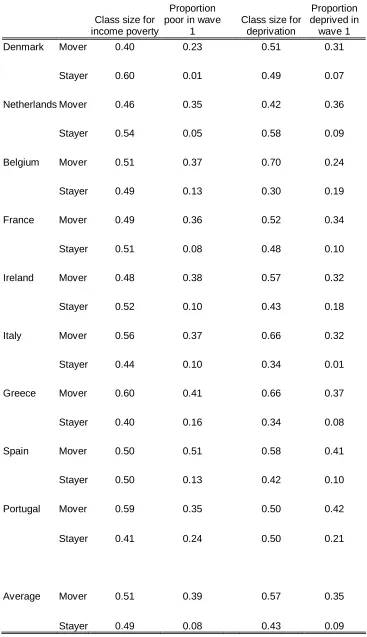
focus on the parameters of the model. In Table 5 we set out, for both types of dynamics, the size of the

mover/stayer classes and the proportion poor/deprived in wave 1. For income poverty the proportion

of movers varies between 0.40 in Denmark to 0.60 in Greece with a tendency for stayers to be a

minority in Northern European countries and a majority in Southern European countries such as Italy,

nine countries. The mover rates range from 0.42 in the Netherlands to 0.70 in Belgium. On average the

proportion of movers is higher for deprivation than income poverty with the respective figures being

0.57 and 0.51. In both cases the mover rate is higher in the South than in the North with the figures for

the former being 0.56 and 0.60 respectively for poverty and deprivation compared to 0.47 and 0.54.

Thus stability is generally greater for poverty and deprivation in the Northern countries. However, the

vast majority of estimates are located in a relatively narrow range.15

15

Table 5: Class size of movers/stayers for income poverty/deprivation and initial proportion of non-poverty/non-deprivation

Class size for income poverty

Proportion poor in wave

1

Class size for deprivation

Proportion deprived in wave 1

Denmark Mover 0.40 0.23 0.51 0.31

Stayer 0.60 0.01 0.49 0.07

Netherlands Mover 0.46 0.35 0.42 0.36

Stayer 0.54 0.05 0.58 0.09

Belgium Mover 0.51 0.37 0.70 0.24

Stayer 0.49 0.13 0.30 0.19

France Mover 0.49 0.36 0.52 0.34

Stayer 0.51 0.08 0.48 0.10

Ireland Mover 0.48 0.38 0.57 0.32

Stayer 0.52 0.10 0.43 0.18

Italy Mover 0.56 0.37 0.66 0.32

Stayer 0.44 0.10 0.34 0.01

Greece Mover 0.60 0.41 0.66 0.37

Stayer 0.40 0.16 0.34 0.08

Spain Mover 0.50 0.51 0.58 0.41

Stayer 0.50 0.13 0.42 0.10

Portugal Mover 0.59 0.35 0.50 0.42

Stayer 0.41 0.24 0.50 0.21

Average Mover 0.51 0.39 0.57 0.35

Focusing on initial poverty and deprivation rates for movers and stayers, we find that such rates are

substantially higher for the former. In the first wave the average poverty rate for movers is 0.37

compared to that of 0.11 for stayers. An almost identical position is observed for deprivation with the

corresponding outcomes being 0.35 and 0.11. Clear North-South differences in initial poverty rates are

found for both movers and stayers. For the latter the respective figures are 0.07 and 0.16 and for the

former 0.34 and 0.41. Thus North-South differences in latent poverty rates are influenced both by the

relative proportion of movers and stayers and differences in the initial poverty risk. For deprivation,

however, the latter factor plays somewhat less of a role in South-North difference. Initial deprivation is

on average higher for movers than stayers with the respective figures being 0.39 and 0.31. However,

for stayers the initial poverty rate in Northern countries is actually higher than its Southern counterpart,

the respective figures being 0.13 and 0.10.

Estimated Proportions of True Stability and Change

Before focusing on the relative importance of different types of error, we shall first address the issue of

overall levels of manifest and latent movement and stability. We do so by partitioning observed change

and stability into true and error components using the parameter estimates of the time heterogeneous

mover-stayer model. Using the terminology of Langeheine and Van de Pol (1990) the total proportion of

stability (TOS) is the proportion of cases remaining in their original state throughout the observation

period, expressed as a proportion of the total sample. This includes all those in the stayer categories

who are assumed to exhibit perfect stabilities (PS). Hence TOS indicates true stability. TRS or ‘true

observed stability’ can be thought of as the proportion of TOS that is observed as stability. The

difference between TOS and TRS is error. Observed change can be deconstructed in a similar fashion.

Total change (TOC) indicates true change and it can be calculated as 1- (TOS + PS). TOC can be

partitioned into true observed change TRC and error. TRC is the proportion of true change TOC that is

observed as such. By comparing TRS and TRC to TOS and TOC we can estimate how much error

increases the observed estimates of mobility in our poverty and deprivation transition tables.

In Table 6 we show the results of these calculations. The forst two columns show observed stability

(OBS) and observed change (OBC). The proportion of true stable cases that the model estimates is

equal to perfect stability plus total observed stability (PS + TOS). In the vast majority of countries

observed levels of stability and change for poverty and deprivation are similar, although the poverty

stability rate is generally higher. The average level of observed stability is 0.67 for poverty and 0.63 for

respective figures being 0.71 and 0.68 compared to 0.63 and 0.58. Comparing observed with latent

rates, we find that in every case levels of stability increase significantly when measurement error is

taken into account. In other words the level of mobility is consistently overestimated. Thus the average

levels of latent stability for poverty and deprivation respectively are 0.81 and 0.82, with the difference

that was found at he observed level disappearing. For both poverty and deprivation the Northern

stability rates remain higher with the respective figures being 0.84 and 0.77 and 0.85 and 0.80.

Table 6: Estimated Proportions of True Stability and Change and Poverty/Deprivation Rate in the Poverty/Deprivation Transition Tables

OBS OBC Perfect

stability TOS TRS error TOC TRC error

Perfect stability + TOS

Perfect stability stability + TRS

Denmark Income 0.74 0.26 0.60 0.28 0.14 0.14 0.13 0.07 0.06 0.88 0.74 Deprivation 0.70 0.30 0.49 0.27 0.17 0.09 0.24 0.09 0.15 0.76 0.66

Netherlands Income 0.73 0.27 0.54 0.32 0.19 0.13 0.14 0.08 0.07 0.86 0.73 Deprivation 0.73 0.27 0.58 0.30 0.15 0.16 0.12 0.05 0.07 0.88 0.73

Belgium Income 0.69 0.31 0.49 0.37 0.19 0.18 0.14 0.06 0.08 0.86 0.68 Deprivation 0.63 0.38 0.30 0.57 0.32 0.25 0.13 0.06 0.08 0.87 0.62

France Income 0.7 0.3 0.51 0.33 0.20 0.13 0.17 0.10 0.07 0.84 0.71 Deprivation 0.7 0.3 0.48 0.40 0.18 0.22 0.11 0.04 0.07 0.88 0.66

Ireland Income 0.7 0.3 0.52 0.23 0.15 0.08 0.25 0.16 0.09 0.75 0.67 Deprivation 0.63 0.37 0.43 0.42 0.20 0.22 0.15 0.05 0.10 0.85 0.63

Italy Income 0.63 0.37 0.44 0.37 0.18 0.19 0.18 0.09 0.10 0.81 0.62 Deprivation 0.55 0.45 0.34 0.43 0.20 0.23 0.23 0.11 0.12 0.77 0.54

Greece Income 0.61 0.39 0.40 0.34 0.19 0.15 0.26 0.12 0.14 0.74 0.59 Deprivation 0.52 0.48 0.34 0.40 0.16 0.24 0.27 0.10 0.16 0.74 0.50

Spain Income 0.63 0.37 0.50 0.25 0.11 0.14 0.24 0.10 0.14 0.75 0.61 Deprivation 0.59 0.41 0.42 0.46 0.16 0.30 0.12 0.04 0.08 0.88 0.58

Portugal Income 0.65 0.35 0.41 0.35 0.23 0.12 0.24 0.13 0.11 0.76 0.64 Deprivation 0.65 0.35 0.50 0.29 0.14 0.15 0.21 0.10 0.11 0.79 0.64

For income poverty, in every case the observed stability is below the true rate. The level of error

ranges from 12% in Portugal to 19% in Italy and the true level of stability ranges from 74% in Greece

perfect stability plus TRS equals or comes close to observed stability with the average percentage

difference being less than one per cent. Thus almost all unsystematic error is observed as change.

While the observed results suggest levels of change in Denmark and Greece of 26% and 39%

respectively, the corrected estimates indicate levels of 13% and 26% respectively. Since the correction

for error is always in the same direction, the pattern whereby more change is observed in the Southern

than Northern European countries is maintained, although Ireland moves nearer to the Southern

pattern.

The pattern for deprivation is remarkably similar. The observed level of stability ranges from 73% in the

Netherlands to 52% in Greece while the corresponding figures for the corrected estimates are 88% in

the Netherlands and 74% in Greece. Similarly, in each case perfect stability plus TOS equals or comes

close to observed stability with the average difference equalling one per cent. Thus once again the vast

bulk of error is counted as change. There is again a tendency for less change to be observed for the

Northern European countries, although in this case Denmark constitutes an exception. Taking

measurement error into account suggests that deprivation is more stable than income poverty in

Ireland, Spain and Portugal. In Denmark and Italy the opposite is true and in Netherlands, Belgium,

France and Greece there is little difference.

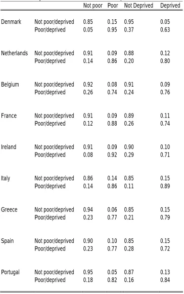
Distinguishing Types of Measurement Error

In fact, the more notable contrasts between income poverty and deprivation dynamics relate not to

overall levels of mobility and stability but to difference in types of mobility and stability. The modal

response probabilities in the diagonal of the reliability matrices set out in Table 7 provide separate

estimates of reliability for the poor and the non-poor and deprived/non-deprived. Comparing the poor

and non-poor we find that for the Northern European countries there is no clear pattern of differentiation

between the types of reliability. Both range between 0.85 and 0.95 with the average level of

misclassification being 0.13 for the poor and 0.10 for the non-poor. In Northern Europe excluding

Belgium, which is something of an exception, the highest level of misclassification of non-poor as poor

is 0.15 in Denmark and of poor as non-poor is 0.14 in the Netherlands and Italy. The Southern

European countries display a somewhat different pattern with the level of reliability being significantly

lower for poor as opposed to non-poor. Thus while the reliability levels for the former vary between 0.77

and 0.86 for the latter they are found in the range running from 0.86 to 0.95. In other words, while

percentages for misclassification of the non-poor ranges between 0.05 and 0.14. The contrast is even

sharper if we exclude Italy.

Table 7: Reliability rates for movers for income and deprivation

Not poor Poor Not Deprived Deprived

Denmark Not poor/deprived 0.85 0.15 0.95 0.05

Poor/deprived 0.05 0.95 0.37 0.63

Netherlands Not poor/deprived 0.91 0.09 0.88 0.12

Poor/deprived 0.14 0.86 0.20 0.80

Belgium Not poor/deprived 0.92 0.08 0.91 0.09

Poor/deprived 0.26 0.74 0.24 0.76

France Not poor/deprived 0.91 0.09 0.89 0.11

Poor/deprived 0.12 0.88 0.26 0.74

Ireland Not poor/deprived 0.91 0.09 0.90 0.10

Poor/deprived 0.08 0.92 0.29 0.71

Italy Not poor/deprived 0.86 0.14 0.85 0.15

Poor/deprived 0.14 0.86 0.11 0.89

Greece Not poor/deprived 0.94 0.06 0.85 0.15

Poor/deprived 0.23 0.77 0.21 0.79

Spain Not poor/deprived 0.90 0.10 0.85 0.15

Poor/deprived 0.23 0.77 0.28 0.72

Portugal Not poor/deprived 0.95 0.05 0.87 0.13

Poor/deprived 0.18 0.82 0.16 0.84

The pattern for deprivation dynamics is a good deal different. The average error level for the deprived is

twice that for the non-deprived, with the respective figures being 0.24 and 0.12. This contrast is

particularly striking in the five Northern European countries where the exit from deprivation error level is

four times that of the corresponding entry to deprivation rate, with the respective figures being 0.27 and

0.07. Here we find that, while the error rates for the non-deprived range between 0.10 and 0.05, for the

deprived they are significantly higher with a minimum value of 0.20 and a maximum of 0.37 . In the

Southern European countries the differences are a good deal more modest with a rate of 0.19 for the

deprived and one of 0.15 for the non-deprived.

Observed and Latent Income Poverty and Deprivation Persistence

A full discussion of the similarities and difference between income poverty and deprivation dynamics

requires that we simultaneously take into account differences in the size of the latent mover-stayer

classes, the initial poverty/deprivation rates, and corrected transition rates for stayers. All of these

elements are reflected in the estimates, set out in Table 8, of the latent risk of being in

poverty/deprivation in subsequent waves given that one is poor/deprived in wave one. These figures

can be compared with the corresponding observed figure in Table 3. There we observed that

persistence was somewhat stronger for income poverty than for deprivation. For the former the

conditional poverty rates declined gradually from 0.69 in the second wave to 0.59 in the fifth wave,

while for the latter the corresponding figures were 0.64 and 0.57. Having corrected for measurement

error, however, we find the opposite is true. Thus the successive conditional rates of 0.84, 0.76. 0.70,

0.66 for income poverty are in each case lower than the corresponding deprivation rates of 0.86, 0.80,

0.73 and 0.69. France, Ireland and Spain are characterised both by very high levels of latent

deprivation persistence and by larges gaps between the observed and latent values. However, with this

exception, one is more struck by the level of uniformity across dimensions and countries than by

Table 8: Latent risk of poverty/deprivation after poverty/deprivation in

wave 1

Latent Risk of poverty in subsequent waves after wave 1 in poverty

Latent Risk of deprivation in subsequent waves after wave 1 in deprivation

P(1/2) P(1/3) P(1/4) P(1/5) P(1/2) P(1/3) P(1/4) P(1/5)

Denmark 0.78 0.70 0.70 0.70 0.76 0.67 0.57 0.58

Netherlands 0.86 0.75 0.66 0.57 0.86 0.82 0.74 0.63

Belgium 0.90 0.77 0.73 0.72 0.92 0.83 0.79 0.69

France 0.78 0.74 0.67 0.65 0.94 0.88 0.83 0.81

Ireland 0.85 0.80 0.71 0.67 0.99 0.97 0.84 0.83

Italy 0.85 0.78 0.72 0.63 0.79 0.71 0.61 0.52

Greece 0.84 0.77 0.72 0.67 0.73 0.64 0.62 0.60

Spain 0.81 0.70 0.69 0.63 0.96 0.90 0.88 0.87

Portugal 0.89 0.80 0.74 0.67 0.82 0.74 0.70 0.65

Average 0.84 0.76 0.70 0.66 0.86 0.80 0.73 0.69

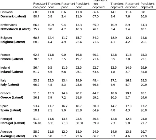
In Table 9 we compare the distribution of observed and latent income poverty and deprivation

distributions across time. However, in this case, rather than using a count of the number of years out of

five in poverty, we have followed Fouarge and Layte (forthcoming) in constructing poverty profiles that

allow us to examine both the persistence and recurrence of poverty by distinguishing between:

• The persistent non-poor – never poor during the accounting period • The transient poor - poor only once during the accounting period.

• The recurrent poor – poor more than once but never longer than two consecutive years.

• The persistent poor – poor for a consecutive period of at least three consecutive years.

In the vast majority of cases the observed poverty and deprivation profiles are similar. This is also the case for the latent profiles. For both the poverty and deprivation profiles movement is substantially

lower when account is taken of measurement error. The average level of persistent non-poverty is 58%

for the observed level and 66%for the latent. The corresponding figures for deprivation are 55% and

67%. Persistence on the other hand is much higher at the latent than the observed level, with the

respective figures for poverty and deprivation being 18% v 23% and 17% v 23%. It is the intermediate

states of transient and recurrent poverty that are substantially overestimated. For poverty the observed

level of 24% is twice that of the corresponding latent figure. For deprivation the gap is even wider with

level of observed non-poverty persistence ranges from 69% in Denmark to 51% for Portugal. The

corresponding range for the latent estimates is 81% in Denmark to 56% in Greece. The level of

observed persistent poverty ranges from 11% in Denmark to 24% in Portugal compared to 11% and

30% for latent persistence. Combining the transient and recurrent categories we obtain observed

figures ranging from 20% to 28% compared to latent figures of 8% to 16%.

Table 9: Latent and observed income and deprivation profiles Persistent non-poor Transient poor Recurrent poor Persistent poor Persistent non-deprived Transient deprived Recurrent deprived Persistent deprived

Denmark 68.6 11.8 8.6 11.0 66.4 14.1 11.4 8.0

Denmark (Latent) 80.7 5.8 2.4 11.0 67.0 9.4 7.6 16.0

Netherlands 66.4 10.9 9.4 13.3 65.9 10.9 8.9 14.3

Netherlands (Latent) 75.2 3.8 4.7 16.3 76.1 3.4 2.4 18.1

Belgium 60.3 12.4 11.7 15.7 54.2 18.9 12.1 14.8

Belgium (Latent) 68.3 4.4 4.9 22.4 71.6 4.1 4.2 20.1

France 62.5 11.8 9.0 16.8 60.1 12.8 11.8 15.3

France (Latent) 70.5 6.3 3.5 19.7 71.4 3.5 3.0 22.1

Ireland 56.4 9.5 11.6 22.5 52.7 12.5 14.9 19.9

Ireland (Latent) 61.7 6.5 6.8 25.1 63.6 1.8 3.7 31.0

Italy 53.3 13.5 13.4 19.9 48.4 17.1 16.1 18.3

Italy (Latent) 66.7 4.5 5.3 23.6 66.5 6.9 5.7 20.9

Greece 51.5 13.3 14.9 20.2 44.7 18.0 19.1 18.1

Greece (Latent) 56.1 7.9 7.2 28.8 59.2 10.5 5.7 24.6

Spain 53.4 11.7 16.2 18.7 50.9 14.7 17.3 17.2

Spain (Latent) 58.1 7.1 9.0 25.8 64.9 4.8 4.3 26.0

Portugal 51.4 11.6 13.5 23.5 50.5 12.8 12.8 24.0

Portugal (Latent) 56.48 6.11 7.10 30.31 59.9 7.3 5.0 27.7

Average 58.2 11.8 12.0 18.0 54.9 14.6 13.8 16.7

Average (Latent) 66.0 5.8 5.7 22.6 66.7 5.7 4.6 22.9

The pattern for deprivation is broadly similar. At the observed level the proportion entirely avoiding

error are 76% in the Netherlands and 59% in Greece. Observed persistence levels run from 8% in

Denmark to 24% in Portugal compared to their latent counterparts of 16% in Denmark and 31% in

Ireland. Once again combining the categories involving movement, we find that the observed range of

20% in the Netherlands to 37% in Greece suggests much higher levels of deprivation dynamics than

the corresponding latent figures of 6% for the Netherlands and 16% for Greece.

The overall profiles for both observed and latent are remarkably similar for both poverty and

deprivation. The marginally higher level of persistence for poverty at the observed level disappears with

correction for measurement error. Reflecting the pattern of reliability coefficients, some modest

differences are observed between Northern and Southern countries. For the former the numerical

superiority of the persistent poor over the persistently deprived at the observed level – 16% v 14% - is

reversed at the latent level with the relevant figures being 19% v 21%. In the South, on the other hand,

persistent poverty is higher at both observed and latent levels - 21% v 19% and 27% v 25%. Denmark it

should be noted constitutes something of a deviant case. In the case of income poverty correcting for

measurement error leads to a significant increase in persistence avoidance of poverty but to no change

in the level of persistent poverty. In the case of deprivation, however, we observe precisely the

opposite. The fact that measurement error has such radically different consequences for these

dimensions is consistent with the fact that the relationship between income poverty and deprivation has

generally been found to be exceptionally weak in Denmark. The other striking exception is Ireland

where the reduction in the numbers mobile produced by correction for measurement error is

substantially greater in the case of deprivation than income poverty. France and Spain also display les

movement at the latent level for deprivation than for poverty. However, there is nothing in our findings

to suggest that our conclusions regarding differences in the determinants and consequences of the

different forms of deprivation would be affected if we could substitute the latent variables for the

Conclusions

In this paper we have sought to establish if earlier findings relating to the relationship between income

poverty and deprivation persistence could be due to failure to take measurement error into account.

These had suggested that different forms of persistence are tapping related but distinct dimensions that

display somewhat different patterns of socio-economic variation and have significantly different

consequences for outcomes such as subjective economic strain. Earlier work had also suggested that

the pattern of relationships involving deprivation conformed much more closely to our prior notions of

what we might expect from an indicator that is successfully tapping exclusion from a minimally

acceptable standard of living due to lack of resources. Our objective in this paper has been to establish

whether such findings could be accounted for by the fact that deprivation persistence was being

measured with a great deal more accuracy than income persistence.

In order to address this question we applied a model of dynamics incorporating structural and error

components. This model performs equally well in accounting for poverty and deprivation dynamics. Our

analysis shows a general similarity between error corrected poverty and deprivation dynamics. In both

cases all error is captured as change and we substantially overestimate mobility. Where differences do

arise between poverty and deprivation patterns, the tendency to overestimate mobility tends to be

greater in the case of deprivation rather than poverty. This is related to the fact that the proportion of

movers tends to be significantly higher in the case of deprivation. In particular, total avoidance of

income poverty is more frequent than the corresponding situation relating to deprivation.

Distinguishing between different types of reliability, we find that by far the largest component of error is

associated with overestimation of probability of exiting from such states. There is some North-South

variation with the differential between error rates for income poor and non-poor groups being a good

deal sharper in the Southern European. Thus exit rates for the poor are particularly overestimated in

these countries. The opposite holds true for deprivation with the tendency to overestimate exits from

deprivation being somewhat higher in the Northern countries.

Focusing on poverty and deprivation profiles we observe remarkable similarity across

dimensions at both observed and latent levels . In both cases levels of poverty and

deprivation persistence are higher at the latent than the observed level. However, while in the South

poverty is more persistent than deprivation at both observed and latent levels, in the North this pattern

though found for the observed data is reversed at the latent level. However, there is no evidence that

a consequence of differential patterns of reliability, Taking measurement error into account seems more

likely to accentuate, rather than diminish, the contrasts highlighted by earlier research. Since

longitudinal differences relating to poverty and deprivation cannot be accounted for by measurement

error, it seems that we must accept that we are confronted with issues relating to validity rather than

reliability. In other words, although income poverty and deprivation are substantially correlated, even

where we measure them over reasonable periods of time and allow for measurement error they

continue to tap relatively distinct phenomenon. Thus if measures of persistent poverty are to constitute

an important component of EU social indicators, as suggested by Atkinson et al (2002), a strong case

can be made for including parallel measures of deprivation persistence and continuing to explore the

References

Ashworth, K., Hill, M., & Walker, R. 1994, "Patterns of Childhood Poverty: New Challanges for Policy", Journal of Policy Analysis and Management, vol. 13, pp. 658-680.

Atkinson, A. B., Cantillon, B., Marlier, B., & Nolan (2002), Social Indicators: The European Union and Social Inclusion. Oxford: Oxford University Press.

Bane, M.J. and D.T. Ellwood. (1986), “Slipping in and out of poverty: the dynamics of poverty spells”, The Journal of Human Resources, 12,pp.1-23

Basic, E and Rendtel, R. (2004), Latent Markov Chain Analysis of Income States with the Euroean Community Household Panel: Empirical results on Measurement Error and attrition Bias, Paper presented at the 2nd International Conference of ECHP Users-EPUNet, Berlin, June 23-26. Breen, R and Moisio, P. (forthcoming), ‘Overestimated Poverty Mobility: Poverty Dynamics Corrected

for Measurement Error’, Journal of Economic Inequality

Buhman, B., Rainwater, L., Schmaus, G., & Smeeding, T. 1988, "Equivalence Scales, Well-being, Inequality and Poverty: Sensitivity Estimates Across Ten Countries Using the Luxembourg I ncome Study Database", Review of Income and Wealth, 34, pp. 115-142.

Dewilde, D. (2204), ‘The Multidimensional Measurement of Poverty in Belgium and Britain: A Categorical Approach, Journal of Social Indicators.

Duncan, G., Gustaffsin, B, Hauser, R., Schmaus, G, Messinger, H, Mufferls, R., Nolan, B, Ray, J, (1993), ‘Poverty dynamics in Eight Countries’, Journal of Population Economics, 6:2, pp.-34 Fouarge, D. and Layte, R.(forthcoming), The Duration of Spells of Poverty in Europe’ Journal of Social Policy

Gordon, D. (2002): Measuring Poverty and Social Exclusion in Britain: The Dynamics of Poverty Workshop, Central European university, Budapest, May 24-25.

Langeheine, R. and van de Pol, F. (1990), ‘A Unifying Framework for Markov Modelling in Discrete Space and Discrete Time’, Sociological Methods and Research, 18, pp.416-441

Langeheine, R. and van de Pol,, F. (2002), ‘Latent Markov Chains’, in Hagenaars, J. A. and Mc Cutheon, A.L., Applied Latent Class Analysis, Cambridge, Cambridge University Press

Layte, R. and Whelan, C. T. (2003), "Moving In and Out of Poverty", European Societies, vol. 5, no. 2,

pp. 167-191.

Lazarsfeld, P.F., & Henry, N.W.(1968), Latent Structure Analysis. Boston: Houghton Mifflin

Leisering, L and S Leibfried. (1999), Time and Poverty in Western Welfare States: United Germany in Perspective. Cambridge MA: Cambridge University Press.

Mack, J. & Lansley, S. 1985, Poor Britain Allen and Unwin., Londo

McCutheon, A. and Mills, A. (1998), ‘Categorical Data Analysis; Log-Linear and Latent Class Models, in Scarborough, E. Tannenbauum, E., Research Strategies in the Social Sciences, Oxford, Oxford

University Press

Moisio, P (2004), Poverty Dynamics According to Direct, Indirect and Subjective Measures. Modelling Markovian Processes in a discrete time and space with error, STAKES Research Report 145, Helsinki Moisio, P. (forthcoming), ‘ A Latent Class Application to the Multidimensional Measurement of Poverty’,

Quantity and Quality-International Journal of Methodology

Muffels, R. & Fouarge, D. (2004),’ The Role of European Welfare States in Explaining Resources Deprivation’. Social Indicators Research, 68: 299-330

Pérez-Mayo, J. Measuring Deprivation in Spain. IRISS Working Paper series No. 2003-09. 2003. Perry, B. (2002), ‘The Mismatch Between Income Measures and Direct Outcome Measures of Poverty’,

Social Policy Journal of New Zealand, 19:101-127

Rendtel, U., Langeheine, R and Bernstein, R,. (1998), The estimation of poverty dynamics using different household income measures’, Review of Income and Wealth, 44:81-98

Ringen, S. (1988), "Direct and Indirect Measures of Poverty", Journal of Social Policy,

vol. 17, pp. 351-366.

Van de Pol, F. and de Leeuw, J. (1986), “A atent Markov Model to Correct for Measurement Error”, Sociological Methods and Research, 15, 1:118-141

Vermunt, J. K. (1997), LEM: A General Programme for the Analysis of Categorical Data, Tilburg University

Watson, D. 2003, "Sample Attrition Between Wave 1 and 5 in the European Community Household Panel", European Sociological Review, vol. 19, no. 4, pp. 361-378.

Watson, D. & Healy, M. 1999, Sample Attrition Between Waves 1 And 2 in the European Community Household Panel, European Commission, Luxembourg, 118/99.

Ringen, S. (1987), The Possibility of Politics. Oxford: Clarendon Press.

Whelan, C. T., Layte, R., Nolan, B. and Maîltre, B. (2001), "Income, Deprivation and Economic Strain: An Analysis of the European Community Household Panel," European Sociological Review Vol. 17 (No.

4): 357-372.

Whelan, C. T., Layte, R., Maître, B., & Nolan, B. 2003, "Persistent Income Poverty and Deprivation in the European Union: An Analysis of the First Three Waves of the European Community Household Panel", Journal of Social Policy, vol. 32, no. 1, pp. 1-32.

Whelan, C.T, Laute, R. and Maitre, B. (2004) ‘Understanding the Mismatch between Income Poverty and Deprivation: A Dynamic Comparative Analysis’, European Sociological Review