Learning with Similarities on Subsets

(1)

Learning with Similarities on

Subsets

Avraham Pinchas Ruderman

A thesis submitted for the degree of

Doctor of Philosophy

of The Australian National University

(2)

(3)

iii

Except where otherwise indicated, this thesis is my own original work.

Avraham Pinchas Ruderman

(4)

(5)

Acknowledgements

I would like to thank my supervisor Mark Reid, for his guidance and advice through-out my PhD. I would also like to thank the rest of my supervisory panel, Stephen Gould and Bob Williamson for their time and advice.

I would like to thank the many people I interacted with at NICTA for sharing their knowledge with me. Particularly, I would like to thank Darío García-García for many interesting conversations and a number of collaborations, Nicolás Della Penna for sharing his knowledge of Economics and Machine Learning with me and for en-couraging me to keep going when I was ready to quit my PhD, Edwin V. Bonilla for always sharing with me the Bayesian perspective on every topic, and Tiberio Caetano for many interesting philosophical discussions. I would also like to thank everyone who took part in the reading group at NICTA, I learned a great deal from those sessions.

I would also like to thank Barry, Myriam and Min for taking me in as an intern at CISRA during my PhD and for everything they taught me.

The PhD journey for me was just as much a mental challenge as it was a technical one. I would like to thank those whose friendship helped keep me sane throughout the PhD: Paul, Suranga and Shamin from the chess club and Aaron and Brit for the many entertaining games nights. BCB. I would also like to thank Zoe for her friendship and for helping me out so much when I was getting started in Canberra.

I would like to thank my parents for instilling in me curiosity and independence.

Most of all though, I thank my wife Priya, for her never ending support for me in every way during the course of my PhD.

Finally, I would like to thank the Australian National University, NICTA, and the Australian tax payers for supporting me financially during my PhD.

(6)

(7)

Abstract

Many machine learning models are based on similarities between new examples and previously observed examples. Such models are extremely flexible and can adapt to a wide range of tasks. However, if examples are composed of many variables, then even if we collect a large number of examples, it is possible that no two examples will be significantly similar. This, in turn, means that a learning algorithm may require an unreasonably large number of examples to learn such models.

In this thesis, however, we show that a small modification of such models, using sim-ilarities on subsetsof the variables, rather than similarities on all variables, can allow us to learn using fewer examples and without a large increase in the required com-putational complexity, if two conditions hold. The first condition is that similarities on certain subsets are indicative of the targets. The second condition is that the vari-ables can be partitioned into a small number of groups such that the varivari-ables within each group are highly dependent.

For instance, suppose we want to learn a classifier which takes images of handwritten digits and outputs the digit drawn in the image. We would like to learn such a classifier based on example images. If we measure similarity to a new example image, depicting a 4, it is quite possible that many of the most similar previous images we have depict a 9. However, if we measure similarity on certain subsets of the pixels, for example, on the region corresponding to the top third of the image, then on this subset of the pixels, it is unlikely that an image depicting a 4 will be similar to an image depicting a 9. For such a task, a learning algorithm based on measuring similarities to previous examples would be able to learn a more accurate classifier, from fewer examples, by using similarities on subsets.

But how can the learning algorithm efficiently find suitable subsets of variables on which to measure similarity? This seems like a daunting task, as the number of possible subsets grows exponentially in the number of variables. In this thesis, we suggest that if similarities on certain subsets are indicative of the targets, and if the variables can be partitioned into a small number of groups, such that the variables within each group are highly dependent, then one can find appropriate subsets on which to measure similarity, by considering combinations of groups of highly de-pendent variables. The small number of groups leads to a small number of subsets we need to consider and hence to a manageable computational effort. The high dependence of the variables within each group allows us to achieve much of the re-duction in the number of examples that can be achieved by measuring similarities on subsets, even though we are only considering a small portion of all possible subsets.

(8)

(9)

List of Figures

1.1 An example of a handwritten digit and target output . . . 1

1.2 Two example images with high overall similarity, for which the appro-priate output is different. . . 2

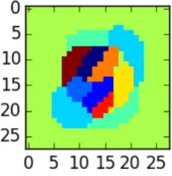
1.3 Similarity on a subset. The subset on which similarity was measured, the examples on this subset, and the difference on this subset. . . 3

1.4 A partition of the variables, for images of handwritten digits, into 10 groups of highly dependent variables. . . 4

2.1 Sample observations from the MNIST dataset. . . 14

2.2 A visualisation of a linear predictor for the MNIST dataset which achieves an accuracy of approximately 92% on the test set. The vector for each class is normalised and below it is displayed an example input from the class. . . 16

3.1 The 14 (out of 16) functions on{0, 1}2that can be represented as linear functions. . . 24

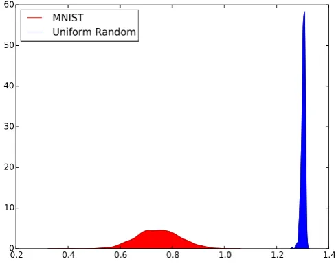
4.1 Distances to nearest neighbours on MNIST vs on randomly sampled points from the unit sphere . . . 50

5.1 Binary MNIST digit . . . 60

5.2 Similarity on a Subset of Size 3 . . . 61

5.3 Similarities onkgroups . . . 63

6.1 Comparison of tradeoffs of number of clusters vs reconstruction error on different sets. . . 74

6.2 A partition of the variables for the MNIST task into k = 10 groups using thek-means algorithm on variables. . . 77

7.1 The graph of the (scaled) Epanechnikov kernel, max 0, 1 u2 _{. . . 88}

7.2 Graph of sigmoid function 1 1+eu2 2 . . . 89

(14)

(15)

Chapter1

Introduction

Suppose we would like a computer program that takes images of handwritten digits and, for each image, or at least for most of the images, outputs the digit that is depicted in the image, as illustrated in Figure 1.1. One possible approach is to collect many example images of handwritten digits, together with the identity of the digit drawn in each image, and then have another program which, using the examples, finds a suitable program that performs well on this task.

Algorithms that take examples of input and appropriate output, and try to pro-duce programs with similar input-output behaviour, are called supervised learning algorithms. An algorithm that takes examples and produces a program is referred to as a learner, while the program it outputs we will refer to as a predictor. It is often useful to think of the learner as producing a model of the input-output behaviour by fitting a number of parameters in a statistical model. Thus, we will also refer to a predictor as afitted model, to the learner as afitting procedure,and to the model, before the parameters are fit, simply as amodel.

One common family of models are those in which the output for each new example depends on its similarity to all previously observed examples. It has been shown that such models can capture almost any input-output relationship of interest given a sufficient number of examples (Györfi et al., 2002). However, if the examples are high-dimensional, that is, if each example is composed of many variables, then there

Figure 1.1: An example of a handwritten digit and target output

“9”

(16)

[image:16.595.171.386.193.251.2]

Figure 1.2: Two example images (left and centre) with high overall similarity, for which the appropriate output is different (4 and 9 respectively). The image on the right depicts the difference between the other two images where for each pixel, white corresponds to no difference and red and blue intensity to the size of difference at

that pixel.

can be so many significantly different examples, that a new example is unlikely to be significantly similar to any example we previously observed (Bengio et al., 2007b). This problem can be formalised as a worst case analysis, often referred to as “the curse of dimensionality,” showing that even if we assume that similar inputs have similar appropriate outputs, the number of examples we need to fit a model could grow exponentially with the number of dimensions (Györfi et al., 2002).

For many tasks that we would like to build models for, the examples are composed of many variables; for example, the image in Figure 1.1 is composed of 784 variables, one real value for the greyscale intensity of each of the 784 pixel in that make up the image. How can we learn models in such situations using a reasonable number of examples?

One possible approach is to measure similarities between examples on subsets of the variables. The advantage of this is that models based on similarities on subsets require fewer examples to learn. For instance, the example in the centre of Figure 1.2 has one of the highest levels of similarity to the example on the left, out of a collection of 60,000 examples of handwritten digits. If we collected many more examples, then eventually we would likely get to a stage where the most similar examples all had the label “4”, but the number of examples we may need until we get to that point may be very large.

However, with the same number of examples, but measuring similarity on the subsets of the pixels depicted in Figure 1.3, the image depicting a 4 and the image depicting a 9 no longer look similar. In fact, on the same subset there are many example 4s that are very similar, but very few 9s.

More generally, if examples are composed of many variables but similarities on cer-tain subsets of the variables are informative about the target, then learning can be done using far fewer examples, by building models based on similarities on these subsets.

(17)

[image:17.595.209.430.191.237.2]

3

Figure 1.3: Similarity on a subset. The subset on which similarity was measured (left image, white pixels) and the examples constrained to having nonzero values only on this subset (two centre). The image on the right depicts the difference between the two centre images where for each pixel, white corresponds to no difference and red

and blue intensity to the size of difference at that pixel.

the number of possible subsets to consider in high dimensions is large, in fact, it is exponential in the number of dimensions. How can we efficiently find suitable subsets on which to measure similarity?

This is the problem this work tries to address and, informally, our main claim is this:

For high-dimensional tasks, if similarities on certain subsets of the variables are highly indicative of the output, and if the variables can be partitioned into groups consisting of highly dependent variables, then we can learn accurate models using significantly fewer examples and without paying a large computational price, by learning with similarities on subsets.

We will precisely define all the terms in the above claim, and make the claim more specific later.

For instance, Figure 1.4 depicts a partition of the variables in images of handwritten digits into a small number of groups containing highly dependent variables. Our claim is that if similarity on certain subsets are highly indicative of the target, and if we can find such a grouping so that the variables within each group are highly dependent and the number of groups is small, then we can learn using fewer ex-amples and using a reasonable amount of computation by considering subsets that are formed as unions of groups of highly dependent variables. Because the variables in each group are highly dependent, we do not pay a large price in terms of the number of examples we need to measure similarity on unions of these groups, and because the number of groups is small, the computational effort of searching through combinations of such groups is also small.

(18)

[image:18.595.217.339.158.283.2]

Figure 1.4: A partition of the variables, for images of handwritten digits, into 10 groups of highly dependent variables.

these pixels may give rise to a subset of pixels thatishighly predictive. An exception to this is the work of Livni et al. (2013) in the context of learning polynomials which does not take a greedy approach based on the supervised objective. Instead, Livni et al. (2013) gradually grow larger and larger subsets, but at every stage find a com-pact representation of the features allowing efficient learning. Indeed, in this sense, our work is closely related to that of Livni et al. (2013).

The remainder of this section gives a detailed breakdown of the chapters in this thesis. Roughly speaking, in Chapters 2, 3, and 4 we introduce the necessary back-ground and explain the problem we are trying to address: learning with similarities in high dimensions. Then, in Chapters 5 and 6 we present our approach: learning with similarities on subsets, where the subsets are composed of groups of highly dependent variables.

1 .

1 Thesis Outline

Chapter2: Background on Supervised Learning and Linear Models

Supervised Statistical Learning. Our focus will be on supervised learning tasks and so in Chapter 2 we describe this class of tasks. In a supervised learning task, we are given pairs of example inputs and appropriate outputs

(x1,y1), . . . ,(xn,yn)

and our task is to fit a model that predicts an appropriate output for each new ex-ample input. More specifically, we describesupervised statistical machine learning tasks

(19)

§1.1 Thesis Outline 5

want to make predictions about are sampled from the same distribution. This “stat-istical” assumption allows us to say something about future expected performance of a predictor on new examples, based on the performance of the same algorithm on previously observed examples.

Linear Models. A common family of machine learning algorithms used for super-vised learning tasks are those based on linear models. These models form the basis for many of the models commonly used today (Shalev-Shwartz and Ben-David, 2014) and will also form the basis of the models in this thesis. Linear models are convenient to analyse mathematically and convenient to deal with computationally. In Chapter 2 we review some well-known results about learning linear models.

Chapter 3: Efficient Learning of Linear Models on Large Sets of Features

Linear models on the original variables may not be very expressive. In particular, there are many functions which cannot be well approximated by linear functions. However, by mapping the original variables to a new set of variables, or features, a linear model using certain sets of features can approximate almost any function of interest. This approach allows us to build very expressive models while allowing us to use analyses and algorithmic approaches developed for learning linear models.

The models we will be dealing with in this thesis can be viewed as linear models on very large sets of features. For example, we will consider linear models on the set of features that can be expressed as similarities to templates, or previously observed examples. In this case, the number of potential templates is as large as the number of different possible examples. How can we deal with such large linear models without using large amounts of computation?

Learning with Large Sets of Features Under L2_, _L1_{, and} _L• _penalties. _{In Chapter}

3 we will review algorithms for efficiently learning linear models on large sets of features. For each such model, the particular algorithms we can use will depend on the penalties or restrictions on the norm of the weights in the linear model. We will review algorithms for learning under L2_, _L1_{, and} _L• _{penalties or restrictions on the}

weights in the model.

• A penalty based on the L2 norm of the weights allows us to deal with certain large sets of features using what is known as the kernel trick (Schölkopf and Smola, 2002).

• A penalty based on theL1_{norm of the weights allows us to}_select_{a small subset} of the features without losing much accuracy (Hastie et al., 2009).

• A restriction on the L• _{norm of the weights allows us to} _{randomly sample} _a

(20)

Penalties based on theL2_{norm of the weight will be important to us, since in Chapter} 4 we will compare some of the models we propose to models based on Reproducing Kernel Hilbert Spaces (RKHS), which rely heavily on the kernel trick to learn linear models on very large sets of features (Schölkopf and Smola, 2002).

Penalties based on the L1 _{norm of the weights will be important for some of the} models we develop in this thesis, for which we will want to select features to use in our model from a large set of features. In such cases, a penalty based on the

L1 _{norm of the weights is a convenient way of expressing preference for selecting a} small number of features.

Restrictions on the L• _{norm of the weights will be important for almost all of the}

models in this thesis since the models are all based on similarities to randomly sampled templates. Under a restriction on the L• _{norm of the weights, we can}

sample features while guaranteeing, with high probability, that we do not lose much through working with this sample of features, as compared to the full set of features. In Chapter 4 we will indeed exploit this idea to express our models as approximating

distribution dependentmodels, rather than simply beingsample-dependentmodels.

We believe some of the results we present in Chapter 3 regarding learning under

L• _{norm restrictions, are new and of independent interest. The results generalise}

those of the Random Kitchen Sinks framework (Rahimi and Recht, 2008) and justify learning with L1 _and_L2 _{norm penalties on the weights of the sampled features.}

Chapter4: Similarities to Templates as Features

In this thesis, we study models based on similarities to templates. What can be said about such models? How do they relate to other models such as nearest neighbours and kernel methods? We try to address these questions in Chapter 4.

Similarities to Templates as Features. In Chapter 4 we expand on the results of Balcan and Blum (2006), who previously studied models based on similarities to templates. In particular, we study models of the form

f(x) =

Z

f x;x0 a x0 dP x0

where Pis the distribution over inputs andfis some function that captures

similar-ity between inputs which satisfies|f(x;x0)|1 for allx,x0_{. For example, a common}

similarity function is the Gaussian Radial Basis Function (RBF) applied to the differ-ence ofxandx0

f x;x0 =exp⇣ g x x0 2⌘

wheregis a parameter with highergcorresponding to a similarity that decays more

(21)

is adaptive, and learning consists of trying to fit a under the constraint that it is

bounded, i.e., sup_x0|a(x0)|Bfor someB. The size ofBgives us a measure of model complexity. Intuitively, if the densitydPis spread out across the space, corresponding to many possible example inputs, then B will need to be quite large in order to compensate for the small values ofdP.

This family of models depends on the true distribution of the inputs, P(X), which

we do not know. However, because a is bounded, we can use randomly sampled

examples, sampled according to P, and for a large enough sample, with high prob-ability, get approximately the same results.

We use our generalisation of the Random Kitchen Sinks framework to derive some new results regarding learning with similarity functions. Some of the results of Bal-can and Blum (2006) Bal-can then be seen as special cases of our generalised framework for learning under a restriction on the L• _{norm of the weights. We believe this}

con-nection between Random Kitchen Sinks and Learning with Similarity Functions is new and may be of independent interest.

The Curse of Dimensionality. The motivation for studying models based on sim-ilarities on subsets is what is often referred to as “the curse of dimensionality,” the large number of examples often required for learning in tasks where the example are composed of many variables (Györfi et al., 2002; Bengio et al., 2007b). For such tasks, many significantly different examples are possible, and so for some such tasks, a ran-domly sampled new example is unlikely to be similar to any previous example, even among a large collection of previous examples. This then motivates the remainder of the thesis, in which we will develop methods for learning with similarities on subsets, which can, for certain tasks, allow us to achieve high accuracy using fewer examples.

Template-Dependent Similarities. We focus on models based on similarities on subsets. We will formulate these models in the more general framework of “learning with template-dependent similarities,” a framework which we develop at the end of Chapter 4.

The work of Balcan et al. (2008) introduced learning with multiple similarity func-tions, which allows one to adapt the similarity function as part of the learning process similarly to the Multiple Kernel Learning framework of Lanckriet et al. (2004). How-ever, in such models, the similarity is fixed across all the examples. This corresponds to an underlying assumption that the same similarity function is appropriate for all examples. However, learning with template dependent similarities allows one to adapt the similarityper template. In particular, we will study models of the form

f(x) =

Z

fx0 x,x0 dP x0

=

Z J

Â

j=1

(22)

where fx0(x,x0) = Â_jJ₌₁f_j(x,x0)a_j(x0)and where f₁, . . . ,f_J are different similarity functions.

We developed this framework of learning with template dependent similarities for use with learning our models based on similarities on subsets. This work is still incomplete. However, we have included the work on learning with template de-pendent similarities in this thesis as it could be relevant to future work on learning with similarities on subsets, and since it may be of independent interest. For instance, this framework could facilitate the study of algorithms that choose, per template, the precision at which to measure similarity.

Chapter5: Similarities on Subsets: A Simplified Analysis

In Chapter 5, we start to put forward our main claim — that similarities on subsets can be used to lower sample complexity without paying a large price in computa-tional complexity, under certain conditions — and start arguing in favour of this. We start with a very restricted setting to make the analysis simpler. In particular, we assume that the examples are from_{0, 1_}d, that is, that they are binary vectors of lengthd, and that the similarity function being used is the indicator of equality

f(x;t) =

(

1 ifx=t

0 otherwise.

These assumptions simplify the analysis by reducing many of the calculations to counting of certain simple quantities.

In the context of these assumptions, a common model that has been studied in the theoretical literature, and which can be learned using smaller samples in high di-mensions, is the k-junta model (Blum and Langley, 1997). A k-junta model makes predictions based on a subset of the variables, where the subset is of size k ⌧ d. We slightly modify this model for our purposes, and then explain the reduction in sample complexity that such models give. However, we also point out the high computational complexity, per example, of learning such models, given current al-gorithms. This sets up the main problem we are trying to solve: Learning in high dimensions can have a high sample complexity, and though the sample complexity can possibly be lowered by learning with similarities on subsets, this can lead to high computational costs.

(23)

1. Any model that could be expressed in terms of similarities on subsets of sizek

can also be expressed in terms of similarities on subsets composed ofkgroups.

2. If the number of groups is small, then the number of combinations, and there-fore the number of subsets on which to measure similarity, is small, leading to a significant reduction in computational complexity per example.

3. If the variables within each group are highly dependent, then the sample com-plexity is not greatly increased by considering similarities onk groups of vari-ables rather than k variables. In particular, similarities on k groups can still lead to significant reductions in sample complexity relative to similarities on all variables.

We note here that a complete analysis would include a quantification of the tradeoff of the sample andoverall(not just per example) computational complexity. However, while we have informal arguments about this tradeoff, a formal analysis has been left as future work.

While the simplifying assumptions we made in the chapter lead to a simpler analysis, they are also unrealistic. In particular, for many domains, the inputs are continuous, and using an indicator of equality as our measure of similarity would lead to an extremely high sample complexity. In addition, the assumption that the variables within each group only take onexactlyone of a small number of values is unlikely to hold in practice. This then motivates the next chapter, where we extend the ideas to continuous variables with continuous similarities.

Chapter6: Continuous Similarities on Subsets

In Chapter 6, we take the ideas from Chapter 5 — of finding large groups of highly dependent variables and considering similarities on combinations of these — and attempt to extend them to domains with continuous variables and to models based on continuous similarity functions such as the Gaussian RBF similarity function

f(x,t) =exp gkx tk

2

ktk2 !

.

In particular, we suggest an analogous framework to that of Chapter 5, in which

• the size of a clustering achieving a certain level of error on a subset is taken as a measure of complexity of learning models on such a subset;

(24)

• we build models based on similarities on combinations of groups of highly dependent variables.

We note here that the extension we present in the chapter is incomplete and some of the parts have been left as future work. In particular, while we extend the con-cepts and some of the algorithms, the extension of the analysis to the continuous case has been left as future work. However, we do discuss a possible direction for extending the analysis by normalising the similarities to each example so that they haveL1 _{norm 1. In addition, the algorithms we propose, both for finding groups of} highly dependent variables and for combining such groups into subsets on which to measure similarity, currently use auxiliary objectives and heuristics and could likely be improved by using more appropriate objectives.

Finally, we provide a review of other approaches to learning features based on sub-sets of the variables and discuss their relation to the framework in this thesis.

Chapter7: Conclusion

In chapter 7, we discuss future directions in which the work in this thesis could be extended. We also put forward a number of conjectures in relation to the neural network models. In particular, we show that features in neural network modelscan

(25)

§1.2 Main Contributions 11

1 .

2 Main Contributions

In this section, we specify what we believe to be the main contributions of this thesis.

• A framework for learning with similarities on subsets in high dimensions that allows the learner to reduce the sample complexity by measuring similarities on subsets but avoids a large computational cost by exploiting dependencies among variables. This framework is the topic of Chapters 5 and 6.

• A generalisation of the Random Kitchen Sinks framework of Rahimi and Recht (2008) and a formal connection of this framework to the framework of Balcan and Blum (2006) for learning with similarity functions. The generalisation of the Random Kitchen Sinks framework appears in Subsection 3.2.2. The connec-tion with the framework of Balcan and Blum (2006) in Subsecconnec-tion 4.1.1.

(26)

1 .

3 Notation

Some notation we will use throughout this thesis:

• Upper case letters will typically be used for random variables, e.g.,X,Y.

• P(A)for the probability of event A occurring, and overloading notation, ifX

is a random variable,P(X)for the distribution ofX

• Efor expectation

• Eˆ for empirical expectation. That is, for a function f and an i.i.d. sample

X1, . . . ,Xm with the same distribution asX, ˆE[f(X)]:= _m1 Âmi=1 f(Xi)

• ^ and _ will denote logical conjunction and disjunction respectively. That is, the expression p1^p2 is true if p1 and p2 are true and false otherwise. The expression p1_p2is true if p1or p2are true and false otherwise.

• I_pfor indicator variable, where pis a predicate. That is,I_p=

(

1 if pis true 0 else

• We will sometimes also writeI(p)in place ofI_p.

• Zfor the set of integers

• Z 0 for the set of nonnegative integers

• O(f(n))for the set of functionsg(n)for which there exists ann ₂ Z ₀ and a

C>0, such thatg(n)_C· f(n)for alln>n0

• W(f(n))for the set of functions g(n)for which there exists ann₂ Z ₀ and a

C>0, such that f(n) C·g(n)for all n>n0

(27)

Chapter2

Background on Supervised

Learning and Linear Models

The problem setting that we assume throughout this thesis is that of supervised stat-istical machine learning, which we review in Section 2.1 of this chapter. The models we construct throughout this thesis will be cast and analysed as linear models. Thus, in Section 2.2 of this chapter we review algorithms for learning linear models as well as known results about the number of examples and time needed for such algorithms to learn.

2 .

1 Supervised Statistical Machine Learning

One way to specify the behaviour of a computer program is by specifyinghowto per-form a desired task. However, there are instances where we do not ourselves know how to perform the desired task. Further, even in instances where we know how to perform the task we might not be able to express our knowledge as instructions for a computer. An alternative approach is to specifywhatthe desired output of the pro-gram should be by providing examples of inputs and desired outputs. The field of

supervised statistical machine learning(Vapnik, 1998) studies algorithms for producing programs in such a way, based on examples of inputs and desired outputs, under the assumption that the examples are all chosen randomly according to the same fixed distribution and that the performance of the program will be evaluated on examples drawn from the same fixed distribution. This allows us to analyse the expected performance of a program on new, unseen examples, based on its performance on examples we have seen.

2.1.1 A Concrete Example

Suppose we desire a program that takes digital images of handwritten digits and outputs an integer corresponding to the digit that has been written. While most

(28)

Figure 2.1: Sample observations from the MNIST dataset.

humans are able to perform this task, specifying to a computer how to perform this task is difficult. One approach to the problem is to collect many examples of human-labeled handwritten digits, and then feed these to a supervised learning algorithm. Such an algorithm takes these examples as input and outputs a program that is able to recognise new handwritten digits with high accuracy. This approach led to the production of the now famous MNIST dataset (LeCun et al., 1998). A number of examples from the MNIST dataset are presented in Figure 2.1.

2.1.2 The Formal Setting

Formally, we will assume that there is a set of possibleinputs,X, and a set of possible

outputs, Y. We will also assume that there is a joint distribution P over X ⇥Y and that we are givenmpairs of inputs from X and targets fromY

(X1,Y1), . . . ,(Xm,Ym)

with each pair (Xi,Yi), 1  i  m sampled independently according to P. We will

refer to each of these points as an observation, and will refer to them collectively as thetraining set. Further, we will assume we are given aloss function `: _Y _⇥_Y _!R.

A loss function lets us specify how undesirable different errors are.

We will call an algorithm that takes themsamples and outputs a function f :X !Y as alearning algorithmand will refer to the output of such a learning algorithm f as a

predictor. We will measure the quality of a predictor using its expected loss on a new sample,

L(f) =E[`(f(X),Y)]. (2.1)

We shall refer to this quantity in equation 2.1 as thetrue risk of f. Given a training set(x1,y1), . . . ,(xm,ym), we shall refer to the quantity

ˆ

L(f) =Eˆ [`(f(X),Y)] = 1

m m

Â

i=1

`(f(xi),yi)

as theempirical riskof f .

An example of a loss function is thezero-one loss

`(yˆ,y) =

(

0 if ˆy=y,

(29)

§2.1 Supervised Statistical Machine Learning 15

If the outputs come from a discrete set, we shall refer to the task as a classification

task. In this case, the zero-one loss penalises a predictor for any incorrect output and penalises all incorrect outputs equally. Another common loss is thesquared loss

`(yˆ,y) = (yˆ y)2.

This loss is often used when the outputs are real valued, in which case the setting is calledregression.

2.1.3 ERM and Penalised ERM

Perhaps the most common class of learning algorithms are those based on empirical risk minimisation (ERM) or penalised ERM (Vapnik, 1998). An ERM algorithm con-siders a set of candidate predictorsF and returns a predictor

ˆ

f 2argmin_f₂_F 1

m m

Â

i=1

`(f(xi),yi).

That is, an ERM algorithm returns a predictor ˆf ₂ _F achieving the minimum loss on the dataset of any f 2 F. Penalised ERM allows us to associate a cost W(f)to each predictor f 2F. Thus, a penalised ERM algorithm with penaltyWreturns

ˆ

f 2argmin_f₂_F 1

m m

Â

i=1

`(f(xi),yi) +W(f).

There are a number of advantages to using penalised ERM:

• Certain sets F of predictors contain so many diverse predictors that there is a high probability that a predictor output by an ERM algorithm may have high true risk, despite having low risk on a training set. Such a situation is referred to asoverfitting. By adding a penalty W, penalised ERM can allow us to learn even with such F. In fact, by scaling W, we can control the exact tradeoff between empirical risk, and model complexity.

• We may prefer certain predictors in F, for instance, because they are faster to compute on new examples or because they consume less memory. Penalised ERM can allow us to specify our preference for such predictors.

Penalised ERM is also referred to as regularised ERM. We note that both ERM and penalised ERM transform a supervised learning problem into an optimisation prob-lem.

(30)

[image:30.595.94.465.167.246.2]

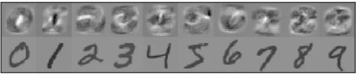
Figure 2.2: A visualisation of a linear predictor for the MNIST dataset which achieves an accuracy of approximately 92% on the test set. The vector for each class is

norm-alised and below it is displayed an example input from the class.

models that do not include the data generating distribution. We also note that pen-alised ERM is closely related to regularisation of ill-posed problems in optimisation (Tikhonov and Arsenin, 1977) where a regularisation term is added to an ill-posed problem leading to a unique solution and helping with the numerical stability of the optimisation procedure.

2 .

2 Linear Models

This section provides a basic review of a family of models called linear models. Linear models are both widely used in practice and are well understood theoretically (Shalev-Shwartz and Ben-David, 2014; Mohri et al., 2012). In this thesis, we will formulate most of our models as linear models. This will allow us to build on the many results and algorithms for learning such models.

For an observation x 2 Rn, a linear predictor f with parameters w ₂ Rn makes a

prediction based on the inner product

f(x;w):=_hx,wi.

For binary classification with classes 1 and 1, this prediction can be converted to a binary value by returning the sign of the prediction sign(f(x;w)). For targets in

Y =Rk, a matrixW ₂Rk⇥nis used for prediction

f(x;W) =Wx.

For classification withkclasses, we can convert the output of a linear predictor withk

targets to a class by taking the index with the highest predicted value argmax_ifi(x;W),

where fi is thei-th component function of f. Figure 2.2 offers a visualisation of the

parametersW of a linear predictor with accuracy of 92% on the MNIST task. In the visualisation, we treat the weights for each class as an image, with a weight corres-ponding to each pixel in the image.

(31)

§2.2 Linear Models 17

throughout this thesis. We will introduce the necessary concepts when the need arises.

We note here that in practice, an intercept term bis usually added in linear models so that they take the form

f(x;w):=hx,wi+b.

This bias term can be incorporated into the previous definition by appending a con-stant 1 to each vectorx and appendingbtow,

hx,wi+b=_hx˜, ˜w_i where ˜x = (x1,x2, . . . ,xn, 1) and ˜w= (w1,w2, . . . ,xn,b).

Below we will consider penalising the norm of the weightsw. We note that the bias term is typically not included in the penalty.

In the remainder of this section, we review some of the many results about the statistical and computational properties of algorithms for learning linear models.

2.2.1 Learning Algorithms

A common family of penalties used for linear models are those based on theq-norm of the weights which we now define:

Definition 2.1. Fixd 2 Z>0. Forq 2 [1,•), Theq-normof a vector x 2 Rd, denoted

kxkq, is defined by

kxkqq := d

Â

j=1

xj q.

For q=•, we define

kxkq =max_j xj .

Linear predictors can be learned using penalised ERM, where the penalty is an in-creasing function Rof aq-norm of the weightsw, for someq₂[1,•]

argmin

w2Rd

1

m m

Â

i=1

`(hw,xii,yi) +R

⇣ kwkq

⌘ .

we will also refer to such penalties as Lq _penalties _as _k·k

q is the usual norm on the

space Lq_{(Rudin, 1987).}

(32)

losses and with convex penalty terms (Shalev-Shwartz and Ben-David, 2014; Mohri et al., 2012; Hastie et al., 2009).

In Section 2.2.3 we review known results regarding the computational complexity of learning linear models and in Section 2.2.4 we review known results regarding the sample complexity of learning linear models.

2.2.2 Approximation

Linear predictors on their own are very limited in the relations they can model. A well known example of this is the inability of a linear predictor to represent the XOR function inR2,

f(x1,x2) =sign(x1x2)

as we discuss in Section 3.1. More generally, linear predictors cannot capture interac-tions between variables, referred to as higher-order predicates by Minsky and Papert (1969).

However, as we will see in Section 3.1, we can map observations to another vector space such that in this new space, a linear predictor can model a much larger number of relations. In fact we can map to a space where linear models can be used to approximate almostanyrelation that may be of interest.

2.2.3 Computational Complexity

The problem of finding a linear predictor with the lowest misclassification loss for a given dataset is known to be NP-hard (Ben-David et al., 2003). That is, unless

P= NP, a proposition largely believed to be false amongst computer scientists, there exists no polynomial time algorithm which works across all datasets for finding the best linear predictor.

On the other hand, under a convex loss such as the square loss, `2, finding a linear predictor achieving a loss close to that of the ERM linear predictor can be done efficiently, and similarly for penalised ERM, as long as the penalty function is also convex (Mohri et al., 2012; Shalev-Shwartz and Ben-David, 2014).

Even if we are interested in finding a predictor with low misclassification loss, we can replace the misclassification loss with a convex loss which upper bounds it. Under this new loss, which is referred to as aconvex surrogate loss, the best linear predictor can be found efficiently (Bartlett et al., 2006). Since the surrogate loss upper bounds the misclassification loss, the misclassification error of the optimum found under the convex surrogate loss will be less than the surrogate loss.

For binary classification with outputy, and for a predictor with raw prediction ˆy2R,

(33)

§2.2 Linear Models 19

• Logistic loss: `(y, ˆy) =log 1+e yyˆ = yyˆ+log 1+eyyˆ

• Hinge loss: `(y, ˆy) =max(0, 1 yyˆ)

• Square loss: `(y, ˆy) = (y yˆ)2

Learning a linear predictor under a convex surrogate loss can be done very efficiently and the high speed with which linear models can be learned has greatly contributed to their popularity (Mohri et al., 2012; Shalev-Shwartz and Ben-David, 2014; Hastie et al., 2009).

2.2.4 Sample Complexity

When learning using penalised ERM, we find a predictor that has low empirical risk on thetraining set, but what can we say about the true risk of this predictor on unseen examples? We formulate the answer to this question in terms of the probability of large deviations between the empirical risk, observed on the training set, and the

true risk, or expected risk on unseen examples. The number of samples required to guarantee that with probability at least 1 d, the deviation of the empirical risk from

the true risk is less thane, is referred to as theuniform deviations sample complexityand

is denoted by m(d,e). The number of samples required to give a similar guarantee that an algorithm outputs a predictor with error not more than e larger than that

of the best predictor will be referred to as the excess risk sample complexity. In this thesis when we saysample complexitywithout qualifying, we will be referring to the uniform deviations sample complexity.

A bound on the uniform deviations sample complexity implies a bound on the excess risk sample complexity. To see this, note that if for all predictors in some classF, the deviations of the empirical risk from the true risk are less thane/2, then the predictor

ˆ

f chosen by ERM will have error at most e larger than f⇤, the best predictor in F, since

E

h

`⇣fˆ(X),Y⌘i E[`(f⇤₍_X₎_,_Y_{)] =}_Eh_`⇣_fˆ₍_X₎_,_Y⌘i _Eˆ h_`⇣_fˆ₍_X₎_,_Y⌘i

+Eˆ h`⇣fˆ(X),Y⌘i E[`(f⇤(X),Y)] +Eˆ [`(f⇤₍_X₎_,_Y_)] _Eˆ _[_`₍_f⇤₍_X₎_,_Y_)]

 e₂ +0+e

2

= e.

(34)

For learners of linear predictors, in the case of penalised ERM learners based on

p-norms of the parameter vector w, there exists a very clean theory of the sample complexity.

First we will need the following definition for the loss function:

Definition 2.2. A function f :Rn _!Ris L-Lipschitzif

|f(x) f(y)_|_ Lkx yk2 for all x,y2Rn.

and the following definition for the norm:

Definition 2.3. We will say that p,q2(1,•)areconjugate exponentsif 1_p+1_q =1. We

also say that p,qare conjugate if p=1,q=•or p= •,q=1.

Conjugate exponents are often referred to as Hölder conjugates after their use in Hölder’s inequality.

We now state the main result regarding sample complexity of linear predictors that we will use throughout this thesis.

Theorem 2.4. (Kakade et al., 2009, Corollary 4) Suppose that 2  q  • and p is the conjugate exponent of q. Suppose further that kXkp  1 with probability 1 and that ` is an L-Lipschitz loss function. Then the sample complexity of learning a linear predictor with norm_kw_k_q_ B with true risk at mostelarger than the best such w with confidence1 dis

m(d,e)O ✓_L₂_B₂

e2

✓

p+log1

d

◆◆ .

Under the same conditions as above, but with q=1and p =•, we have that

m(d,e)__O

✓_L₂_B₂

e2

✓

logd+log1

d

◆◆ .

The fact that the sample complexity grows quadratically in kwkq, independently of

the dimension d whenq 2 allows us, barring computational difficulties, to learn in very high-dimensional, or even infinite-dimensional, spaces. For the special case

q = 1, the sample complexity grows linearly in log(d) allowing us to learn with

(35)

§2.3 Discussion 21

2 .

3 Discussion

(36)

(37)

Chapter3

Efficient Learning of Linear Models

on Large Sets of Features

As we saw in Chapter 2, the sample complexity of learning linear models is well understood. In addition, many algorithms exist for learning such models efficiently. However, one major drawback of linear models is that they may be very limited in the functions they can approximate. To overcome this limitation, we can map the original inputs to a large set of features, and learn a linear model on this new set of features. With particular choices of features, this can allow us to approximate a much larger set of functions, and ultimately, any function of interest.

However, mapping to very high-dimensional spaces leads to computational chal-lenges. In this chapter, we discuss methods for dealing with these computational challenges under L2_, _L•_{, and} _L1 _{penalties. We believe the result in Theorem 3.3} is new and generalises the theory behind the Random Kitchen Sinks algorithm, for learning linear models in high dimensions under a restriction on the L• _{norm of the}

weights.

In the next chapter, we will focus on a particular family of feature maps, those based on similarities to previously observed examples, and we will use the scheme presen-ted in this chapter, for efficiently learning under an L• _{penalty, to formulate the}

theory there. Then, in later chapters, we will formulate the selection of relevant sub-sets for each template by having a feature corresponding to each possible subset, and then learning under an L1 _{penalty on the weights. Here we will use the ideas about} efficiently learning under L1_{penalty, which we review in this chapter.}

3 .

1 Feature Maps

Linear models, which were discussed in the previous chapter, are very attractive since their properties are well understood theoretically and since, in practice, algorithms

(38)

[image:38.595.164.369.191.390.2]

Figure 3.1: The 14 (out of 16) functions on {0, 1}2 that can be represented as linear functions. The points on each side of a line satisfy the predicate beside the line. On each side of a line the region corresponds to . The illustration is based on a figure in

Minsky and Papert (1969, p. 28).

1 1 x1 constant 0 constant 1 (x1, x2)

= (1,

0)

(x1, x2)

≠ (1,

0)

(x1, x2)

≠ (0,

1)

(x1, x2)

= (0,

1) x2 x1=1 x1=0 x2=0 x2=1 (x1, x2) = (0, 0) (x1, x2) ≠ (0, 0) (x1, x2) =(1, 1) (x1, x2)≠ (1, 1)

for learning linear models tend to require few samples and are extremely computa-tionally efficient when the learning is achieved using a convex loss. However, a major drawback of linear predictors is that they are very limited in the functions they can represent or even approximate. A well-known example of this is the inability of a linear predictor to represent the XOR function on{0, 1}2

f(x1,x2) = (

1 ifx16=x2 0 otherwise.

For a “proof” of this claim, see Figure 3.1 which is based on Section 2.1 of Minsky and Papert (1969). In fact, linear predictors cannot capture interactions between variables, and so, as the dimension dgrows large, they form an exponentially small subset of all possible functions on{0, 1}d (Minsky and Papert, 1969, Section 2.1).

One way to reduce the bias of our learner, while still benefitting from the well-developed theory and algorithms for learning linear predictors, is to map the inputs

X1, . . . ,Xm, from the original spaceX to a new vector spaceX0 using a map

f:X !X0,

and then to learn a linear predictor, using f(X) as our features. We will refer to

f as afeature map, or basis expansion. For certain combinations of feature maps and

distributions, linear models on f(X) may be able to approximate a larger set of

(39)

§3.1 Feature Maps 25

X =_{0, 1_}d, then a linear predictor on the inputs transformed by the feature map

f:{0, 1}d !{0, 1}2d :x7! ⇣I_x₌₍_0,0,...,0₎,I_x₌₍_0,0,...,1₎, . . . ,I_x₌₍_1,1,...,1₎⌘

could represent any function from _X to R. However, in high dimensions, and for

certain distributions, this f could be a very bad choice and could require a huge

number of samples for learning.

3.1.1 Infinite-Dimensional Feature Spaces

The feature mapfmay map to an infinite-dimensional spaceX0. In the last chapter, we only discussed linear predictors on finite-dimensional vector spaces. However, as we saw in Section 2.2.4, the sample complexity for learning under aq-norm penalty with 2 q•was independent of the dimension, and in fact, the same results hold in infinite-dimensional spaces (Kakade et al., 2009). In the case q= 1, the bound on

the sample complexity depended on the dimension d through a logd term. The theory for the case q = 1 can also be extended to infinite-dimensional spaces if the set of features, considered as predictors, have low complexity themselves (Shalev-Shwartz and Ben-David, 2014).

Many classical machine learning algorithms can be viewed as learning linear pre-dictors in high-dimensional or infinite-dimensional spaces. In fact, any learner that outputs a linear combination of models from some class_F, can be seen as learning a linear model over the space spanned byF. For instance:

• Boosting: Boosting algorithms can be analysed as learners of linear predict-ors over the space spanned by a set of base hypotheses (Mason et al., 1999; Friedman et al., 2000).

• Functional Gradient Boosting: Algorithms such as Gradient Boosted Trees are derived as algorithms for learning linear predictors in an infinite-dimensional space of functions (Friedman, 2001).

• Single Hidden Layer Neural Networks: Single hidden layer neural network models are typically learned with a fixed number of neurones. However, re-laxing the hard limit on the number of neurones to an L1 _{norm penalty on the} output weights, leads to a convex formulation of neural networks learning over the infinite-dimensional space, where each dimension corresponds to a hid-den neurone with one of the possible settings of the input to hidhid-den weights (Bengio et al., 2005; Bach, 2014).

(40)

3.1.2 Common Feature Maps

Below we list common families of feature maps which we will encounter throughout this thesis:

• Hand-engineered features

– In the field of Computer Vision, many of the feature maps have been hand-engineered by domain experts. For instance, until recently, many object-recognition algorithms were based on learning linear predictors on sets of hand-engineered features such as SIFT (Lowe, 1999) or HOG (Dalal and Triggs, 2005). Hand-engineered features are common in many other domains as well, and are often a key component in successful machine learning systems (Domingos, 2012).

• Monomials of degree at mostD

– Polynomials have been studied extensively in past centuries. Any poly-nomial of degree D can be expressed as a linear function on the set of monomials of degree at mostD

f(x) =⇣xD1

1 ·xD22 ·...·xdDd

⌘

D1,...,Dd2DD

whereDD =

n

D1, . . . ,Dd 2Z 0:Âdj=1Dj  D

o .

• Order-restricted predicates

– Early models of learning linear combinations of features, considered fea-tures which were limited to depend on at most k of the input variables, called order-restricted predicates. The resulting models were referred to as

order-restricted perceptrons(Minsky and Papert, 1969, p. 12).

• Artificial neurones

– Inspired by early models of biological neurones, a popular choice of fea-tures has been _n

fw(x) =s

⇣

wT_x⌘_:_w₂_Rdo

wheres:R_!Ris some fixed nonlinear function, e.g.,s:x 7!max(0,x).

Linear models based on this set of features have been extensively studied and have also yielded very good results in practice (LeCun et al., 2015).

(41)

§3.2 Kernels, Sampling, Greedy Methods ande-Covers 27

– Certain bases have nice computational properties under an L2 _{penalty, as} we will see in the next section. For inputs in X = R, one such example

is the feature map which gives rise to the Gaussian Radial Basis Function kernel (Schölkopf et al., 2001)

f(x) = (f0(x),f1(x), . . .) wherefj(x) = p1_j_!e

x2

2 xj.

• Distribution-dependent features

– As we will see, it is often advantageous to consider distribution-dependent feature maps. For instance, we may consider a feature map based on a similarity measure f: X ⇥X ! R between examples, where the feature

corresponding to similarity to a point x0 ₂ _X _{is scaled by the probability} dP(x0)of x0. For instance, if the distributionPover X has densityp, then the set of features under consideration is

f ·,x0 _{p x}0 _:_x0 ₂_X _.

We will use feature maps of this type extensively throughout the remainder of this thesis. Under certain penalties and as an approximation of such models, we can take unlabelled examples,x0

1, . . . ,x0J and learn a model on

the features

1

Jf ·,x01 , . . . ,

1

Jf ·,x0J .

All of the feature maps in the above examples map to high or possibly even infinite-dimensional spaces. How can we deal computationally with such large sets of fea-tures? The next section gives a review of approaches for addressing this computa-tional challenge under penalties on theL2_,_L•_{, or}_L1_{norm of the weights.}

3 .

2 Kernels, Sampling, Greedy Methods and

e-Covers

In the previous section, we saw that linear models can be made very expressive by mapping to another feature space. However, many of the feature spaces we would like to map to are very high-dimensional. This leaves us with a computational chal-lenge: How can we efficiently learn linear models in very high dimensions? In this section we review different approaches for efficiently learning linear models under convex losses on large (possibly infinite) sets of features.

(42)

• In Subsection 3.2.2, we review an approach based on randomly sampling fea-tures for learning efficiently under an L• _penalty

• In Subsection 3.2.3, we review two approaches based on greedily selecting fea-tures and usinge-covers for learning efficiently under an L1 penalty

We first present the general formulation of the problem of learning linear predictors in high dimensions under q-norm penalty. We will suppose that we have a set of features indexed byQand a feature mapf:X⇥Q!R. We will assume some fixed

probability measure QoverQ. Forq2{1, 2,•}, and a sample(x1,y1), . . . ,(xm,ym),

we consider the problem of finding a minimiser of

L(w) =

m

Â

i=1

`(f(xi;w),yi) +R

⇣ kwkq

⌘

(3.1)

where Ris a monotone nondecreasing function and where, for finite Q,

f(x;w) =

Â

q2Q

w(q)f(x;q)Q({q}) and kwkqq=

Â

q2Q|

w(q)|qQ({q}). (3.2)

IfQis infinite, then we generalise the above to

f(x;w) =

Z

Qw(q)f(x;q)dQ(q)

and_k·k_qto the usual norm over the space of functions Lq₍_Q_,_Q₎_,

kwkqq=

Z

Q|w(q)|

q_dQ₍_q₎_.

The unconstrained optimisation in (3.1) is often used in practice but is difficult to analyse directly. We will typically analyse the optimisation problem

argmin_w_:_k_w_k_q__B

Â

m

i=1

`(f(xi;w),yi) (3.3)

instead. This is justified by the fact that a solution to (3.1) is also a solution to (3.3) for someB>0. To see this, let B=_kw⇤_k

q, wherew⇤ is a minimiser ofL(w)(if there are

multiple minimisers, with different kw⇤_k

q, choose the one with the minimal kw⇤kq).

If there exists a ˆwwith kwˆkq  B and Âim=1`(f(xi; ˆw),yi) < Âmi=1`(f(xi;w),yi)or

Âm_i=1`(f(xi; ˆw),yi)  Âmi=1`(f(xi;w),yi) andkwˆkq < B, then we would also have L(wˆ)<L(w⇤₎_{, contradicting the fact that}_w⇤ _{is a minimiser of} _L₍_w₎_.

Measure theoretic considerations: We will assume throughout that all functions under consideration are (P⇥Q)-measurable. This can usually be easily justified by

(43)

3.2.1 Kernels Under an L2 Penalty

Consider the objective function when trying to learn using penalised ERM under a penalty term that is an increasing function Rof the squared L2 _{norm of the weights}

L(w) =

m

Â

i=1

`(f(xi;w),yi) +R

⇣ kwk22

⌘

, (3.4)

where f is of the form (3.2). Let

S=span(f(x1), . . . ,f(xm))

be the span of the observed features, and note that we can decompose w into two parts,

w=wS+wS?,

such thatwS lies inSandwS? is orthogonal toS. We then observe that the objective can be rewritten as

L(w) =

m

Â

i=1

`(_hwS,f(xi)i,yi) +R

⇣

kwSk2₂+kwS?k2₂ ⌘

sincew_S? is orthogonal to each of thef(xi)and since

kwk22 =kwSk22+kwS?k2₂+2hwS,wS?i

and _hwS,wS?i = 0. Finally, note that kw_S?k2₂ is always positive, and since R is an increasing function, for anyw, we have

L(wS) L(w).

Thus, the minimiser of L(w) can always be written as a linear combination of the

observed features f(x1), . . . ,f(xn). This result is known as the representer theorem

and was is due to Kimeldorf and Wahba (1970). Let us state the result formally

Theorem 3.1. Let R : R _! Rbe a monotonically increasing function. Then there exists a

minimiser of

L(w) =

m

Â

i=1

`(_hw,f(xi)i,yi) +R

⇣ kwk22

⌘

lying in the span off(x1), . . . ,f(xm).

The above theorem says that there is a solution w to the optimisation problem (3.4) that takes the form

w=

m

Â

j=1

(44)

Replacing w with the expression above, we see that our objective function can be written as

L(w) =

m

Â

i=1

`

m

Â

j=1

aj⌦f xj ,f(xi)↵,yi

!

+R

Â

i

Â

j

ajai⌦f xj ,f(xi)↵

! .(3.5)

Note that this final form is expressed in terms of only inner products between fea-ture vectors at observed points. Thus, if we can efficiently compute inner products (and therefore norms) between feature vectors, then we have reduced our infinite-dimensional optimisation problem to an m-dimensional optimisation problem. The function computing the inner product is usually referred to as akerneland denoted byk(x,x0) =hf(x),f(x0)i, allowing us to rewrite 3.5 in the more concise form

L(w) =

m

Â

i=1

`

m

Â

j=1

ajk xj,xi ,yi

!

+R

m

Â

i=1

m

Â

j=1

ajaik xj,xi

! .

Finding inner product spaces and feature mappings such that inner products between feature vectors can be computed efficiently has been extensively studied (see, for in-stance, Schölkopf and Smola, 2002). This idea of reducing learning in infinite dimen-sions under anL2_{penalty by reformulating the problem as a finite-dimensional one} has been applied to feature maps based on linear threshold functions as well as fea-tures based on Rectified Linear Units. This has been done in the context of Gaussian Processes (see, Neal, 1995), as well as in the context of Support Vector Machines (see, Cho and Saul, 2009).

Advantages

• Exact finite-dimensional representation: Unlike the methods we present for

learning linear predictors in high-dimensional spaces under L• _and _L1 penal-ties, which lead to only approximate minimisers, in the case of learning under an L2 _{penalty with kernels, the objective can be expressed} _exactly _{as a} finite-dimensional problem.

Disadvantages

• Restriction to features with efficiently computable kernels: The above

frame-work only applies to a very small subset of possible feature maps, those for which we can efficiently compute the inner product between two observed fea-ture vectors.

3.2.2 Sampling Under an L• Penalty

(45)

a linear predictor under an L• _{penalty on the weights with respect to}_Q_{. That is, we}

will consider the objective function

L(w) =

m

Â

i=1

`(f(xi;w),yi) +lkwk•

where f is of the form 3.2 and

kwk• =max_q₂_Q |w(q)|.

In the case that Qis infinite, we takekwk• to be the essential supremum ofw with

respect to the measureQ.

As we will see in this subsection, a penalty on the L• _{norm of the weights justifies}

randomly sampling features. In this thesis we will formulate many of our models in the above manner, whereQwill correspond to the set_X of possible examples, Q

will correspond to the marginal distribution, P(X), over inputs, and f(x;q)will be some measure of similarity between x and q. The results in this section show that

for learning a predictor under an L• _{penalty, we can learn a linear predictor on a}

set of features sampled randomly according to Q. When learning using similarity functions, this allows us to view learning with similarities to randomly sampled examples as an approximation to a distribution-dependent model. We explore this idea further in Chapter 4.

In this subsection we will see that under an L• _{penalty on the weights, simply}

sampling features according to the distribution Q and learning a linear predictor on these sampled features can still give almost optimal results with high probability. This is the basis of the Random Kitchen Sinks algorithm of Rahimi and Recht (2008), which is justified by the following lemma:

Lemma 3.2. (Rahimi and Recht, 2008, Lemma 1) Fix d > 0 and w : Q _! R, with

kwk•  B. If q1, . . . ,qK are drawn independently according to Q, then with probability at least1 d, there exists aw˜ :{q1, . . . ,qK}!R, withkw˜k• B such that

r

Eh f(X;w) f˜(X; ˜w) 2i_ pB

K 1+

s 2 log

✓₁

d

◆! ,

where f˜(x;v) = _K1 ÂjK=1w˜ qj f x;qj .

The result in 3.2 means that we can sample featuresq1, . . . ,qKaccording toQand then

learn a linear predictor on the sampled featuresf(·;q1), . . . ,f(·;qK), allowing us to

reduce our learning problem to a K-dimensional one. However, the lemma above only formally justifies learning with an L• _{penalty on the weights of the sampled}

Learning with Similarities on Subsets