R E S E A R C H
Open Access
A distributed approach to the OPF problem
Tomaso Erseghe
Abstract
This paper presents a distributed approach to optimal power flow (OPF) in an electrical network, suitable for
application in a future smart grid scenario where access to resource and control is decentralized. The non-convex OPF problem is solved by an augmented Lagrangian method, similar to the widely known ADMM algorithm, with the key distinction that penalty parameters are constantly increased. A (weak) assumption on local solver reliability is required to always ensure convergence. A certificate of convergence to a local optimum is available in the case of bounded penalty parameters. For moderate sized networks (up to 300 nodes, and even in the presence of a severe partition of the network), the approach guarantees a performance very close to the optimum, with an appreciably fast
convergence speed. The generality of the approach makes it applicable to any (convex or non-convex) distributed optimization problem in networked form. In the comparison with the literature, mostly focused on convex SDP approximations, the chosen approach guarantees adherence to the reference problem, and it also requires a smaller local computational complexity effort.
Keywords: Alternating direction method of multipliers; Augmented Lagrangian methods; Convergence guarantee; Distributed processing; Optimal power flow; Smart grid
Introduction
One of the key aspects of the current research trends for the future smart grid is the possibility of devising dis-tributed algorithms for solving a global problem. This corresponds to the idea of a decentralized access to gen-eration/storage resources, as well as to the much more challenging task of decentralized control.
The typical smart grid problem taken into considera-tion for distributed optimizaconsidera-tion is that of optimal power flow (OPF), that is, the optimal management of electrical power throughout the grid under a number of (electri-cal) constraints (e.g., the satisfaction of a power request from a load, the presence of a dispatchable/non dispatch-able renewdispatch-able generator or of a storage system). The OPF problem, being non-convex in nature in both the target function and the constraints, is very difficult to solve. For this reason, a widely used approach is tomap it into a (somehow) close convex problem, and then solve the convex counterpart by means of distributed meth-ods, e.g., the alternating direction method of multipliers. In this context, semi definite programming (SDP)
relax-Correspondence: [email protected]
Università di Padova, Dipartimento di Ingegneria dell’Informazione, via G. Gradenigo 6/b, Padova, Italy
ations have emerged as a common option, e.g., see Lavaei and Sojoudi et al. [1-4], Lam, Tse, and Zhang et al. [5,6], Dall’Anese and Giannakis et al. [7,8], Gayme and Topcu [9], and Erseghe and Tomasin [10]. One of the limits of this approach lies in the lack of adherence to the original problem, and in fact, optimality of the solution can only be ensured for very specific networks. But complexity is also an issue, since the number of variables involved in the local processing is squared with respect to its natural size. A few other worth mentioning approaches are avail-able from the literature. ˘Sulc et al. [11] exploit the (convex) LinDistFlow approximation as a lower complexity alterna-tive to SDP relaxation. Magnusson et al. [12] avoid SDP relaxation and propose a sequential convex approxima-tion approach, which, however, is known to imply slow convergence speeds. Instead, theconsensus and innova-tionapproach has been applied to the (convex) DC-OPF problem by Hug and Kar et al. [13,14], but the chosen dis-tributed algorithm only provides approximate solutions even in the considered convex scenario.
The kind of approach we follow is alternative to the main trend in the literature, in the sense that we do not consider any convex relaxation and work directly on the
non-convex OPF problem. In this way, we can guarantee adherence to the original problem and develop an algo-rithm which is capable of identifying local minima. This idea was originally exploited in [15] where a distributed algorithm based upon ADMM was proposed. This algo-rithm provided undeniable evidence of the goodness of the intuition but had two major drawbacks. First, opti-mization for speed was cumbersome and required central-izedcoordination. Second, no guarantee on convergence was available, and in fact the algorithm often failed to con-verge. Although the convergence failure did not practically prevent the algorithm output for being usable, conver-gence is an issue that practically limits the algorithm speed.
In this paper, we wish to solve the above cited issues. To simplify system parameters and improve convergence speed, we remap the distributed problem in such a way to reveal the networkpower flow. In the ADMM formulation, the power flow variables are adequately weighted in order to force the algorithm to solve an approximate linear prob-lem in the power flow variables in the first iterations (sim-ilarly to what happens with DC-OPF). The approximation is progressively abandoned in later iterations. This corre-sponds to the practical intuition that a linear power flow exchange problem provides a solution which is close to the optimum (some preliminary results on this aspect were recently presented at an international conference [16]). We also modify the plain ADMM algorithm and reinter-pret it as a non-convex augmented Lagrangian method (see the work of Martinez and Birgin et al. [17,18]) where penalty parameters are constantly updated (increased) to always guarantee convergence. More specifically, a global convergence guarantee is available under the assumption that local solvers are efficient, in the sense that they can guarantee the identification of a (feasible) local minimum. This might not be an easy task in general, but it is a rea-sonable assumption when the number of local variables is controlled. Furthermore, a certificate of convergence to a local optimum is available when penalty parameters are bounded. The kind of coordination involved in this pro-cess is only local and therefore defines a fully distributed algorithm.
The rest of this paper is organized as follows. First, the reference OPF problem is presented and put in a net-worked form readily usable for obtaining a distributed algorithm. Then the distributed approach is discussed in abstract form and its convergence properties proved. Application to the specific OPF problem is then detailed, and the proposed distributed algorithm is finally tested in meaningful scenarios.
The OPF problem
We first introduce the OPF problem in its natural (centralized) formulation.
Standard formulation
Consider an electrical network of N nodes at steady state, where Vi, Pi, and Qi represent, respectively, the local complex voltage, and the node’s active and reactive powers. Assume that, at node i, a local cost is associ-ated to active power production through a cost function fi(Pi). Assume that the electrical neighbors of node i are identified through theneighborssetNi, and that the line admittance Yi,j, j ∈ Ni, is known for each physi-cal connection. Then the standard OPF problem has the form straint in (1) refers to power flow equations (i.e., Kirchoff ’s laws). The remaining constraints are voltage and power constraint limitations, with Vi, Vi, Pi, Pi, Qi, Qi local upper and lower bounds.
For the ease of simplicity here we refer to a basic OPF problem, but additional constraints can be easily added to (1), e.g., power flow constraints on specific lines. Constraints referred to resources such as stor-age systems and renewable generators (dispatchable or not dispatchable) can be included by suitably select-ing the cost factorfi, by introducing proper corrections to the cost function, or by inserting a time variable. Discrete variables can be also included in the prob-lem formulation (e.g., the tap changing of the trans-formers, or the cost to turn on/off a generator), in which case a mixed-integer programming solver will be needed. The results that follow are valid for all the above generalizations.
Region-based formulation
Because of power flow equations in (1), the voltages of interest in regionkare those belonging to set
Vk =
i∈Rk
Ni (3)
whereNi identify the neighbors of nodei. Note that set Vk includes setRkas a subset, as well as all those nodes which belong to neighbor regions and which have a direct connection (edge) with one of the nodes ofRk. Accord-ingly, we identify thelocalvoltage vectorsxkwith entries xk,by
xk=[xk,]∈Vk , xk,=V (4)
and the corresponding constraint region
Xk =
V≤ |xk,| ≤V,∀∈Vk,
Pi≤Pi≤Pi,
Q
i≤Qi≤Qi,
Pi+jQi=xk,i
j∈Ni
Yi,j∗x∗k,j,∀i∈Rk ⎫ ⎬ ⎭
(5)
collecting voltage constraints, active and reactive power constraints, and power flow constraints, and to which we may add any additional constraint of interest. Regions Xk are deliberately chosen to be compact (closed and bounded) in order to strengthen later derivations and results.
Hence, a region-based equivalent formalization for (1) corresponds to the non-convex problem
min k∈R
Fk(xk)
w.r.t.xk ∈Xk,k∈R
s.t.xk,=xh,, ∀∈Vk∩Vh,k,h∈R
(6)
whereR= {1,. . .,R}, function
Fk(xk)=
∈Rk
f(P) (7)
collects local cost functions, and where the constraint is forcing equivalence between duplicated (voltage) vari-ables in vectorsxk.
Capturing the power flow
The formalization given in (6), although correct, is some-how unsatisfactory in terms of the slow convergence speed involved with its distributed implementation, and in terms of the difficulty in optimizing its system parameters
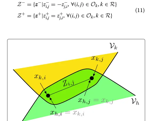
(see [15]). The key point is that we are not using any elec-trical intuition that could help the distributed processing. The intuition we use is illustrated in Figure 1.
The idea with Figure 1 is the following. Consider two neighboring regionsk, and h, and edge(i,j) connecting the two regions, i.e., withi ∈ Rk andj ∈ Rh. It also is {i,j} ⊂Vkand⊂Vh. Then, equivalence between the local variables can be written in the form
xk,i=xh,i xk,j=xh,j
(8)
which is equivalent to the constraint in (6). However, equivalence can be also written in the form
xk,i−xk,j=xh,i−xh,j xk,i+xk,j=xh,i+xh,j
(9)
where the first equivalence captures thepower flow, since the power flowing through line(i,j)is of the formZi,j|Vi− Vj|2, i.e., it only depends on voltage differences as from the first of (9).
The corresponding formulation for the OPF problem can then be compactly written by using sets
Ok =
(i,j) i∈Rk,j∈Ni∩(Vk\Rk)
(10)
collecting in region kthose edges connecting a node of Rkto a node in a neighbor region. By further introducing two auxiliary variablesz−andz+belonging to the linear spaces
Z−= {z−|z−
i,j= −z−j,i, ∀(i,j)∈Ok,k∈R} Z+= {z+|z+
i,j=z+j,i,∀(i,j)∈Ok,k∈R}
(11)
the OPF problem becomes
min k∈R
Fk(xk)
w.r.t.xk∈Xk,k∈R z−∈Z−,z+∈Z+
s.t.ρ (xk,i−xk,j)=z−i,j,
ζ (xk,i+xk,j)=zi,j+,∀(i,j)∈Ok,k∈R
(12)
where two positive constantsρ,ζ are used to differently weigh the power flow constraint onz−(providing conver-gence on an approximate linear problem on power flow variables) from the full equivalence constraint onz+. The linear constraints in (12) can be also expressed in the compact matrix notation
zk=
z−i,j z+i,j
(i,j)∈Ok
=Akxk (13)
where Ak is a sparse matrix of size 2|Ok| × |Vk|. In the typical case of large regions having a few connections with neighbors it is|Ok| |Vk|.
The distributed approach
We now introduce the distributed algorithm in a general and abstract form, in order to assess its properties and capture its structure with a compact notation.
Reference optimization problem
The kind of problem we wish to solve in (12) is a non-convex problem of the form
minF(x)
w.r.t.x∈X,z∈Z s.t.Ax=z
(14)
where x = [xk]k∈R collects all variables,z = [zk]k∈R collects all auxiliary variables,F(x)=k∈RFk(xk)is sep-arable, X = X1× . . .× XR is a Cartesian product, set Z = Z−×Z+is a linear space with associated projec-tor LZ, and A = diag(A1,. . .,AR) has a block diagonal form. The results given in the following further consider Xbounded (as we already assumed), andF(x)continuous. We finally assume that (14) has a solution.
The smoothness of functions involved with the OPF problem ensure that a one-to-one relation exists between local minima of problem (14) and the correspond-ing Karush Kuhn Tucker (KKT) conditions. We have (e.g., see [19])
Theorem 1. (KKT stationary points)
The KKT stationary point conditions associated with the primal problem (14) are given by
0∈∂F(x)+∂ηX(x)+ATλ Ax=z
x∈X , z∈Z, λ⊥Z
(15)
where∂is the proximal sub-gradient operator, and where ηAis the indicator function of setA, withηA(a) = 0 if
a∈Aand+∞ifa∈A. Conditions (15) identify the local
minima of (14).
Augmented Lagrangian formalization
No global minimum ensurance is given in the present con-text, since the Lagrangian associated with problem (14) may suffer of a primal-dual gap. A remedy in this respect is to use a Powell Hestenes Rockafellar (PHR)augmented Lagrangian formulation. TheaugmentedLagrangian asso-ciated with problem (14) can be written in the form
L(x,z,λ,)=F(x)+ηX(x)+ηZ(z)
+λT(Ax−z)+ 1
2Ax−z 2
(16)
where x2 = xTdiag()x is a scaled norm, and where the entries of are strictly positive. In (16), the couple
(x,z)plays the role of primal variables, while (λ,) play the role of dual variables (Lagrange multipliers). Thedual function associated with (16) is
D(λ,)=min
x,z L(x,z,λ,). (17)
The PHR augmented Lagrangian of (16) is well defined, in the sense that it ensures the typical properties of ordi-nary Lagrangians of convex functions, i.e., the zero dual-ity gap property and the applicabildual-ity of a saddle point theorem. The result is given in ([20], Theorem 11.59). Incidentally, we are using a vector of weighting factors instead of a unique multiplication by scalar factor. This, however, does not modify derivation nor the final result.
Theorem 2. (Rockafellar-Wets)
1. Zero duality gapLet(x∗,z∗)be a solution to the primal problem (14), and let(λ∗,∗)be any maximizer of the dual function (17). The corresponding duality gap is zero, that is, we have
2. Saddle pointThe solutions in 1 identify a saddle point of PHR augmented Lagrangian (16), that is
(x∗,z∗)∈argmin
x,z
L(x,z,λ∗,∗)
(λ∗,∗)∈argmax λ,≥0
L(x∗,z∗,λ,). (19)
Conversely, any saddle point (19) identifies a primal and
dual solution, as from 1.
In this context, the search for an optimum point can be turned into the search for a saddle point of the PHR augmented Lagrangian, which is in general more effec-tive in terms of efficiency and speed. However, since only a local optimization point may be available for the first of (19) (because of non-convexity), then onlylocalsaddle points can be practically identified. It is then interesting to observe the following result, which is a straightfor-ward consequence of the fact that local minima/maxima conditions of (19) correspond to KKT stationary point conditions (15), as the reader can easily verify.
Theorem 3.There exists a one-to-one correspondence between local minima of the original problem (14), KKT stationary points (15), and local saddle points of the PHR
augmented Lagrangian in (19).
As a consequence, the search for local minima can be mapped into a search for local saddle points of the augmented Lagrangian.
Alternating direction search for a local saddle point
The search for a local saddle point can be dealt with by using the method of [17] (see also [18]). In our context, the method can be mapped into an alternating direction algorithm of the form
xt+1∈arg min
x∈XL(x,zt,λt,t)
zt+1∈arg min
z∈ZL(xt+1,z,λt,t)
λt+1=λt+Et(Axt+1−zt+1)
(20)
whereEt = diag(t), and wheretis suitably updated at each cycle by guaranteeingt+1 ≥ t. Note that, differ-ently from [17], and similarly to what we have in ADMM, an independent update is used forxtandzt. In turn, dif-ferently from ADMM, the weighting parameters t are updated in order to ensure convergence of the process in a non-convex scenario.
Throughout the process, we assume that the commuta-tion property
LZEt=EtLZ (21)
holds, which corresponds to the request
k,i,j=h,j,i, (i,j)∈Ok,j∈Rh,k,h∈R. (22) We also assume that
λ0⊥Z . (23)
These are light hypotheses guaranteeing that (20) sim-plifies to updates
xt+1∈arg min
x∈XF(x)+ 1
2Ax−(zt−E −1 t λt)2t
zt+1=LZAxt+1
λt+1=λt+Et(Axt+1−zt+1)
(24)
and we also have
zt+1∈Z, λt+1⊥Z (25)
so that the third line in KKT conditions (15) is satisfied throughout the iterative process. Note that the update of xtin the first of (24) corresponds to the parallel of a num-ber of local updates because F is separable, andX is a Cartesian product. In addition, since the full minimum for the first of (24) may be not available, we relax the result by assuming that a local minimum is achieved and that the target function in this local minimumxt+1is smaller than or equal to the function value inxt. Therefore, a reliabil-ity assumption on the local solver is required. Although this might be in general a strong request (e.g., see [21]), especially when the local constraints identify a very small feasibility region, we expect it to be reasonably met when the number of local variables is not too large (i.e., for small regions).
Interestingly, given the fact thatXis bounded, then both sequences{xt}and{zt}are bounded. This may not be the case for{λt}, but it is convenient to force this property by assuming
λt+1=P[λt+Et(Axt+1−zt+1)] (26) with P[λ]= max(λmin, min(λ,λmax))a projection onto a compact box. The reason for this action will become clearer later on in the proof of Theorem 5.
Concerning penalty parameters t, in the centralized fashion of [17] the update criterion ontis of the form
t+1=
t ift+1≤θ t
τt otherwise (27) with constants 0< θ <1 andτ >1, and with
a measure of the primal gap (in infinity norm), in such a way to increase the penalty only if the primal gap is not decreasing sufficiently. The criterion can be also made local. The approach we propose is the following. We first check the primal gap decrease in regionkvia
ˇ k,t+1=
k,t∞1 ifk,t+1≤θ k,t
τk,t∞1 otherwise (29)
with1the all-ones vector, and with
k,t= Akxk,t−zk,t∞ (30)
the local gap. We then select the smallest t+1 ≥ ˇt+1 satisfying (29), which in our context implies
k,i,j,t+1=max requires local message exchanges. With this definition, the update is such that if one value ofk,tgrows to∞, then all the values in the network do so, as it is for the centralized counterpart (27).
The proposed solution is summarized in Algorithm 1.
Algorithm 1:Alternating direction search method
1 Update variablext+1using the first of (24). When a global minimum guarantee is not available, a local minimum must be identified, with the guarantee that the target function is decreased with respect to its value atxt.
2 Update auxiliary variableszt+1=LZAxt+1. 3 Update the Lagrange multipliersλt+1using (26).
4 Update the penalty parameterst+1using (27) or (29)-(31).
Convergence guarantees
The important characteristic of Algorithm 1 is that, in the given scenario, it provides a distributed solution. The main difference with the inspiring technique of [17] lays in the use of an alternating search with respect toxand z(versus the joint minimum search on(x,z)), this being the key point for obtaining adistributedalgorithm. Never-theless, the algorithm always converges (despite the non-convex scenario), and convergence guarantees essentially equivalent to those of [17] can be derived.
We separately treat the case where the penalty con-stant parameters are bounded and the case where they are unbounded. For bounded parameters we have the following result.
Theorem 4.(Bounded penalties)
Consider Algorithm 1, and assume that the sequence of penalty parameters{t}is bounded. We have:
1. Sequences{zt}and{λt}converge to finite values,z∗ andλ∗, respectively.
2. There exists a finite limit point (accumulation point) for the sequence{xt}, and ifATAis invertible then sequence{xt}is further guaranteed to converge to a finite valuex∗.
3. The triplets(x∗,z∗,λ∗), withx∗any limit point of {xt}, satisfy the KKT conditions of (15), hence all limit pointsx∗identify a local minimum to the original problem. Even more, in the limitt→ ∞any triplet(xt,zt,λt)satisfies the KKT stationarity conditions, i.e., identifies a local minimum and satisfies the constraintAxt=zt.
Proof of Theorem 4.Consider that the sequence of penalty parameters{t}is bounded, to havet = ∞for t ≥t0. For both (27) and (29), we have thatt+1 ≤ θ t fort>t0, and thereforeλtis bounded and converges to a finite valueλ∞(also in case the projection (26) is limiting the value to its maximum).
Now, by exploiting equivalencezt=LZAxt, we rewrite the update ofxtin (24) in the form
By then using the shorthand notation
gt = F(xt)+ηX(xt)+1 proved by contradiction. Specifically, ifgtdoes not con-verge to 0 then there exists an infinite sequence for which
also exists an infinite sequence for whichgt ≤ −. By
Since|ζt|is guaranteed to be exponentially decreasing because of the assumptiont+1≤θ t, the above implies g∞ = −∞, hence a contradiction. Therefore, gt con-verges to a finite value, and, as a consequence of (33), the weighted normzt+1−zt2∞ converges to 0, i.e.,zt con-verges to a finite value too. These results justify points 1 and 2.
To conclude with point 3, sincext+1is assumed a local minimum, from (32) we also have, fort>t0,
0∈∂F(xt+1)+∂ηX¸(xt+1)+ATλ∞
+ATE∞(I−LZ)Axt+1
+ATE∞(zt+1−zt)+AT(λt−λ∞)
and since the values on the second and third lines tend to
0in the limit, then in the limit, the KKT stationary point conditions (15) are satisfied.
As a consequence, bounded penalty parameters guaran-tee a convergence of the algorithm to a KKT stationary point, i.e., they imply the identification of a local mini-mum. Note that the result is sufficiently strong also in the case whereATAis not invertible (see second part of point 3). This is an important property since the invertibility ofATAis only ensured for a single-node regions choice Rk= {k}.
The result for unbounded parameters assumes that the ill conditioning associated with very large/infinite values is adequately solved, e.g., by locally normalizing the min-imization in (32) by the maximum penalty valuek,t∞. We have
Theorem 5 (Unbounded penalties). Consider Algo-rithm 1, and assume that the sequence of penalty parame-ters{t}is unbounded. We have:
1. Sequence{zt}converges to a finite value,z∗.
2. There exists a finite limit point for the sequence{xt}, and ifATAis invertible then sequence{xt}is ensured to converge to a finite valuex∗.
Proof. The results in the proof of Theorem 4 can be applied by suitably (locally) normalizing parameters. The kind of replacements we use are
t =⇒ ˜t=
which have the characteristic of providing bounded quan-tities. For both (27) and (29), all entriesk,t are diverging by construction, henceλt˜ is ensured to converge to0in the limit. Convergence is also guaranteed to be exponential, because of the presence of parameterτ >1in the update of penalty parameters. These properties are fundamental and are ensured by use of projection (26). Furthermore,t˜ is guaranteed to converge to the all ones vector1. By then investigating the counterparts to gtandζt, namely,
˜
hold, and we also have that ˜gt converges to 0. Hence ˜
gt converges to a finite value, so that there exist limit points for the sequence{xt}. From (34) we also find thatzt converges to a finite value. This proves the theorem.
Note that Theorem 5, although being able to prove con-vergence of both sequences{xt}and{zt}, cannot guaran-tee that the limit solution is feasible, i.e., it satisfiesAxt= zt. As a matter of fact, in the limit, the minimization in (32) assumes the (approximate) form
xt+1∈argmax
x∈X (I−LZ)Ax
2+ L
ZA(x−xt)2 (35)
which corresponds to an iterative algorithm for perform-ing a projection ofxonto the feasible spaceX∩ {x|Ax= LZAx}, and in this context, the contributionLZA(x− xt)2plays the role of a proximity operator, forcing vicinity to the solution available from the previous step. Therefore, if the algorithm used to solve the local problem (32) is suf-ficiently powerful, then convergence to a feasible point is also ensured in the limit. This is the case, in practice, only for moderately non-convex scenarios.
The distributed OPF algorithm
Algorithm 2:Distributed OPF processing in regionk (tdenotes the iteration number)
1 for t=0to∞do 2 ift=0then
3 Initialize local voltagesxk,0
4 else
5 Update local voltagesxk,tvia
xk,t∈argmin
7 A local minimum must be identified, with the
guarantee that the target function is decreased with respect to its value atxk,t−1. 8 end if
9 Prepare messagesmk,t=Akxk,t
10 ⇒Broadcast messagesmk,tto neighbor regions
11 ⇐Receive messagesmh,tfrom neighbor regionsh
12 Update auxiliary variables via
13
15 Initialize Lagrange multipliersλk,0. If no a
priori information is available, then set them to0.
16 Initialize the local gapk,0= ∞
17 Initialize penalty parametersk,0=1ξ
18 else
19 Update Lagrange multipliers via
λk,t=P¸λk,t−1+diag(k,t−1)(Akxk,t−zk,t)
wherePis a projection onto box [λmin,λmax].
20 Update the local gapk,t= Akxk,t−zk,t∞ 21 Locally update penalty parameters
k,t=
24 Correct local penalty parameters via
k,i,j,t+1=max
Note that two local message exchanges (denoted with arrows) are required in lines 10 to 11 and lines 22 to 23 to exchange, respectively, the updated valuesxk,t(in order to update auxiliary variables) and the temptative penalty parameters updates k,tˇ (in order to make sure that the final update satisfies (21)). In principle, a single message exchange could be obtained by postponing the penalty parameters correction of line 24 after the auxiliary vari-able update in line 13, at the cost of some sub optimality in performance.
Overall, the local processing effort of Algorithm 2 is light. The algorithm complexity is determined by the update ofxtin line 5, which corresponds to a region-based optimization problem, and which can be efficiently solved by state-of-the-art methods, e.g., interior point methods (IPMs). The remaining actions require a limited effort, especially in the standard case where a few connections are active with neighboring regions and auxiliary vectors are short (i.e.,|Ok| |Vk|).
We finally underline that five key parameters are used in Algorithm 2, and these need to be accurately set for good performance. We have:
1. Weighting constantsρandζ(they define matrices Ak, see (12)-(13)). They should be chosen in such a way thatρζ >0, in order to force the algorithm towards an approximate linear solution on power flow variables.
2. Initialization value for penalty parametersξ. It should be set to a small value to guarantee a good algorithm outcome even when starting from a point very far from the optimum.
3. Penalty parameters update constants0< θ <1and τ >1. In order to avoid a rapid increasing behavior on penalty parameters, the constants should be set to values close to 1.
Performance assessment
Description of the scenarios
A power losses minimization problem under voltage and power constraints is considered (i.e.,fi(Pi) =Pi), and the following settings are used in the various scenarios:
1. Networks sizesN=30, 57, 118, and 300 are used. Constraints and load requests are set as from the MATPOWER distribution [26].
2. TheN=123nodes network is used in single-phase fashion. The chosen settings are inspired by [6]. Load requests are set as given in the dataset, and
generating capabilities ranges are added in the form |QG,i| ≤1.2|QL,i|, and0≤PG,i ≤30kW, where the subscriptLstands forload and G for generation. Voltage regulation is applied with0.94≤ |Vi| ≤1.06. 3. A unique network is selected withN =120. The
network is generated as four joint small-world graphs with 30 nodes (to limit the depth of the graph) and rewiring probabilityp=0.4(see also details in [16]). Lines lengths have an exponential distribution with parameterμ=65.86m and a minimum distance set to10m. The impedance value is chosen2.9400+j0.0861/km (class 1,10mm2 cables). Load requests are randomly generated with an uniform distribution in[ 0, 3]kW, and with a uniformcosφwithφ∈[−π8,π8].20%of the nodes are given generation capabilities, randomly distributed in[ 0, 10]kW for active power and
[−20, 20]kVAr for reactive power. Voltage regulation is applied in the range0.9≤ |Vi| ≤1.1.
Region partitioning
Region partitioning is a fundamental aspect for ensur-ing a good performance. Ideally, compact regions with very few outer connections guarantee limited complex-ity, accuracy of the solution, and controlled computational time. In the considered scenarios, region partitioning is chosen in such a way that a unique generator is available in each region, and the region further includes those loads which are electrically closer (in terms of line impedance) to the generator. Since this corresponds to an excessively fine partitioning in Scenario 2), for the IEEE feeder, the region choice is made in such a way that a local controller is placed at each network bifurcation point, and the asso-ciated region corresponds to all those nodes which are electrically closer to it (in terms of line impedance).
Simulation tools
The local optimization problem (see line 5 of Algorithm 2, or see the first of (24)) is solved by using IPOPT [27], an efficient IPM solver which allows a MatLab interface. Although a true optimality guarantee is not available, IPM methods are known to perform very well for OPF kind of problems. MUMPS linear solver is used within IPOPT,
and thewarm start option is used in such a way to start the local minimization process using the solution available from the previous iteration (this reduces computational times). The code is run on a MacBook Air and is written in MatLab [28].
Convergence test in the considered scenarios
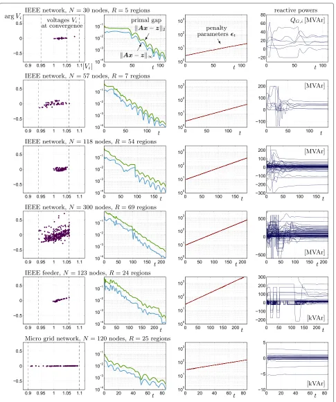
A test on the behavior of Algorithm 2 in the three differ-ent scenarios using the parameters of Table 1 is illustrated in Figure 2. The starting point is chosen to be the all-ones vectorxk,0 = 1, and Lagrange multipliers are initially set to zero,λk,0 = 0. This corresponds to the unavailability of anya prioriinformation on both position and Lagrange multipliers and is therefore a worst case scenario. Iter-ations are stopped (and convergence is declared) when the primal gapAxt−zt∞(infinity norm) reaches 10−4. The maximum values for Lagrange multipliers are set to λmax=103·1,λmin= −103·1.
For the three scenarios considered, Figure 2 shows in the first column the voltagesVi(amplitude and phase dia-gram) at convergence, together with the active voltage constraints. Observe that all voltage limitations are met.
The second column of Figure 2 shows the behavior of the primal gap in norm 2 and norm∞as a function of the iteration numbert. Although the curves are not strictly decreasing, they are clearly diminishing to zero-gap value. The penalty parameters update, illustrated in the third column of Figure 2, shows the ability of (29)-(31) of keep-ing a small gap between maximum and minimum values oft. The fact that the parameters are always increasing is due to the sub optimality of the distributed criterion with respect to the centralized criterion (27) which would be more effective in limiting the increase of penalty parame-ters. Nevertheless, the algorithm converges to points very close to the optimum (see Table 1) despite the very badly chosen initial point. In this respect, the local IPM solvers are fully capable of resolving the limit problem (35) and hence guarantee convergence to a feasible point. Note that the slower convergence is experienced with Scenario 2), i.e., the IEEE feeder withN =123. This is due to the fact that this is the network with highest depth due to its radial structure. This makes the distributed process particularly challenging since agreement must be obtained between regions that are very far one from the other.
Finally, in the fourth column of Figure 2, we provide the locally determined reactive power regulation (QG,istands for reactive power at generators), which show a converg-ing behavior in accordance with the fact that the primal gap is vanishing. A perfectly equivalent behavior is found for active powers (but this is not shown in figure).
Performance evaluation
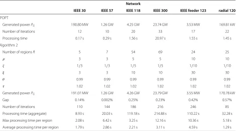
Table 1 Performance starting from a remote point
Network
IEEE 30 IEEE 57 IEEE 118 IEEE 300 IEEE feeder 123 radial 120
IPOPT
Generated powerPG 190.80 MW 1.26 GW 4.25 GW 23.74 GW 3.53 MW 169.81 kW
Number of iterations 12 10 20 33 17 22
Processing time 0.17 s 0.29 s 1.56 s 20.97 s 1.55 s 1.45 s
Algorithm 2
Number of regionsR 5 7 54 69 24 25
ρ 3 3 5 5 10 10
ζ 1/3 1/3 1/5 1/5 1/10 1/10
ξ 3 3 10 10 30 30
θ 0.99 0.99 0.99 0.99 0.99 0.99
τ 1.02 1.02 1.02 1.02 1.02 1.02
Generated powerPG 191.07 MW 1.26 GW 4.26 GW 23.79 GW 3.55 MW 170.78 kW
Gap 0.14% 0.002% 0.25% 0.23% 0.42% 0.57%
Number of iterations 110 144 186 216 246 85
Processing time (aggregate) 8.93 s 20.03 s 119.18 s 214.88 s 110.22 s 32.28 s
Max processing time per region 2.08 s 6.42 s 3.25 s 12.16 s 10.36 s 5.18 s
Average processing time per region 1.79 s 2.86 s 2.21 s 3.11 s 4.59 s 1.29 s
approach of Algorithm 2 is compared with the perfor-mance of a centralized IPOPT solver.
Note that the performance gap with respect to a central solver is always below a 1% error, which is an impres-sive performance considering that we are dealing with a worst case situation, and that we are approaching the problem in distributed form with a severe network parti-tioning. As a matter of fact, the outstanding performance of IPMs is mainly due to their central coordination capa-bilities (e.g., see [15]). Incidentally, we observed that the performance of Algorithm 2 is almost independent of the chosen settings. As a consequence, the performance gap in Table 1 coincides with the ultimate accuracy that could be achieved after thousands of iterations for every studied case.
By inspecting the references, the reader can further appreciate the substantial improvement with respect to the performance of the ADMM-based algorithm of [15], and the sensibly improved network size and partitioning performance with respect to the preliminary algorithm version of [16].
Processing times
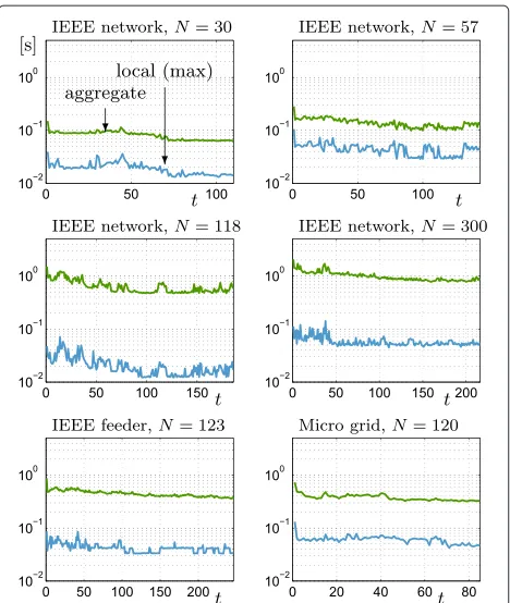
Some information on the processing times involved with Algorithm 2 is given in both Table 1 and Figure 3.
Figure 3 shows, for the six networks under consid-eration, the maximum local processing time and the aggregate processing time per iteration. These are almost constant throughout the iterative process, evidencing the
fact that the processing time is approximately linear in the number of iterations. From Table 1, we can further extract some information on the time needed per region (themax processing time per region), which is in a range between 2 and 13 s, the value being in agreement with the literature on distributed OPF (e.g., see [6]).
Observe that communication delays were not taken into account in Figure 3 and Table 1, and in fact these can be made negligible by choosing a suitable communication technique. High data rate communication standards with associated short packet lengths are to be preferred. This is the case, for example, of broadband power line commu-nication techniques which can guarantee packet lengths of less than a millisecond [29] and which can be deployed in small area applications (e.g., in micro grids). WiMax is a wireless alternative in these scenarios. For wide area applications, instead, optical fiber communications (e.g., gigabit Ethernet) are an appropriate solution.
Conclusions
Figure 2Performance of distributed OPF with IEEE and microgrid networks.
on a point very far from its final destination. The algo-rithm was proven to be efficient and fast and to be also robust with respect to a severe network partitioning. Its
Figure 3Local and aggregate processing times per iteration.
added value of allowing for a full adherence to the original problem since no (convex) approximation is used.
On the applicability side, the distributed algorithm is readily applicable on moderate time scales (tens of sec-onds) and on moderate sized networks (up to 300 nodes) for system optimization purposes, not concerning fast regulation (e.g., fault or protection issues require much faster time scales). In this scenario, the algorithm is also expected to be robust to packet losses, because of its alternating direction structure.
Applicability to larger network sizes, with many loops, and more severe non-convexities is instead out of the scope of the present work. As a matter of fact, the pro-posed alternating direction search allows distributing the processing burden, but might not find an agreement (or it might take too long) in harsh situations. To overcome these difficulties, two strategies can be jointly employed. On the one side, some criteria to determine the opti-mal region partition strategy should be identified. On the other side, some additional coordination between agents should be used, e.g., a proper distributed generalization of the techniques used in the work of Martinez and Birgin et al. [18] which could also be capable of closing the per-formance gap with respect to a centralized solver. Use of recent advances on ADMM accelerated methods and scal-ing techniques (e.g., see [30]) is also an interestscal-ing option but need to be suitably adapted to a non-convex context. These aspects are left for future investigations.
Competing interests
The author declares that he has no competing interests.
Authors’ information
Tomaso Erseghe was born in 1972. He received the Laurea (M.Sc degree) and the Ph.D. in Telecommunication Engineering from the University of Padova, Italy in 1996 and 2002, respectively. Since 2003, he is Assistant Professor (Ricercatore) at the Department of Information Engineering, University of Padova. His current research interest is in the fields of distributed algorithms for telecommunications, and smart grids optimization. His research activity also covered the design of ultra-wideband transmission systems, properties and applications of the fractional Fourier transform, and spectral analysis of complex modulation formats.
Received: 12 December 2014 Accepted: 14 April 2015
References
1. J Lavaei, SH Low, Zero duality gap in optimal power flow problem. IEEE Trans. Power Syst.27(1), 92–107 (2012)
2. S Sojoudi, J Lavaei, inIEEE Conference on Decision and Control (CDC). On the exactness of semidefinite relaxation for nonlinear optimization over graphs: Part I (Florence, Italy, 2013), pp. 1043–1050
3. S Sojoudi, J Lavaei, inIEEE Conference on Decision and Control (CDC). On the exactness of semidefinite relaxation for nonlinear optimization over graphs: part II (Florence, Italy, 2013), pp. 1051–1057
4. R Madani, S Sojoudi, J Lavaei, Convex relaxation for optimal power flow problem: mesh networks. IEEE Trans. Power Syst.30(1), 199–211 (2015) 5. AYS Lam, B Zhang, DN Tse, inIEEE 51st Annual Conference on Decision and
Control (CDC 2012). Distributed algorithms for optimal power flow problem (Maui, HI, 2012), pp. 430–437
6. B Zhang, AYS Lam, A Dominguez-Garcia, DN Tse, An optimal and distributed method for voltage regulation in power distribution systems. To appear in IEEE Trans. Power Syst.
7. E Dall’Anese, H Zhu, GB Giannakis, Distributed optimal power flow for smart microgrids. IEEE Trans. Smart Grid.4(3), 1464–1475 (2013) 8. E Dall’Anese, SV Dhople, BB Johnson, GB Giannakis, Decentralized optimal
dispatch of photovoltaic inverters in residential distribution systems. IEEE Trans. Energy Conv.29(4), 957–967 (2014)
9. D Gayme, U Topcu, Optimal power flow with large-scale storage integration. IEEE Trans. Power Syst.28(2), 709–717 (2013)
10. T Erseghe, S Tomasin, Power flow optimization for smart microgrids by SDP relaxation on linear networks. IEEE Trans. Smart Grid.4(2), 751–762 (2013)
11. P ˘Sulc, S Backhaus, M Chertkov, Optimal distributed control of reactive power via the alternating direction method of multipliers. IEEE Trans. Energy Conversion.29(4), 968–977 (2014)
12. S Magnusson, PC Weeraddana, C Fischione, A distributed approach for the optimal power flow problem based on ADMM and sequential convex approximations. To appear in IEEE Trans. on Control of Network Systems 13. S Kar, G Hug, inPower and Energy Society General Meeting, 2012 IEEE.
Distributed robust economic dispatch in power systems: a consensus + innovations approach (San Diego, CA, 2012), pp. 1–8
14. J Mohammadi, S Kar, G Hug, Distributed approach for DC optimal power flow calculations. arXiv (2014). arxiv.org/abs/1410.4236
15. T Erseghe, Distributed optimal power flow using ADMM. IEEE Trans. Power Syst.29(5), 2370–2380 (2014)
16. T Erseghe, inIEEE International Conference on Smart Grid Communications, 2014. A distributed algorithm for fast optimal power flow regulation in smart grids (Venice, Italy, 2014)
17. R Andreani, EG Birgin, JM Martínez, ML Schuverdt, On augmented lagrangian methods with general lower-level constraints. SIAM J. Optimization.18(4), 1286–1309 (2007)
18. E Birgin, J Martínez,Practical Augmented Lagrangian Methods for Constrained Optimization. (Society for Industrial and Applied Mathematics, Philadelphia, PA, 2014)
20. RT Rockafellar, R Wets, inFundamental Principles of Mathematical Sciences. Variational analysis, vol. 317 (Springer Berlin, 1998)
21. A Castillo, RP O’Neill, Computational performance of solution techniques applied to the ACOPF. Federal Energy Regulatory Commission, Optimal Power Flow Paper.5(2013)
22. RD Christie, Power Systems Test Case Archive. www.ee.washington.edu/ research/pstca
23. WH Kersting, inIEEE Power Engineering Society Winter Meeting, 2001. Radial distribution test feeders, vol. 2 (Columbus, OH, 2001), pp. 908–912 24. Group, D.T.F.W.: Distribution test feeders. ewh.ieee.org/soc/pes/dsacom/
testfeeders 2010
25. GA Pagani, M Aiello, Power grid network evolutions for local energy trading. arXiv (2012). arxiv.org/abs/1201.0962
26. RD Zimmerman, CE Murillo-Sánchez, RJ Thomas, Matpower: Steady-state operations, planning, and analysis tools for power systems research and education. Power Systems, IEEE Trans.26(1), 12–19 (2011)
27. A Wächter, LT Biegler, On the implementation of an interior-point filter line-search algorithm for large-scale nonlinear programming. Math. Program.106, 25–57 (2006)
28. MATLAB,Version 7.13.0.564 (R2011b). (The MathWorks Inc., Natick, Massachusetts, 2011)
29. AR Di Fazio, T Erseghe, E Ghiani, M Murroni, P Siano, F Silvestro, Integration of renewable energy sources, energy storage systems, and electrical vehicles with smart power distribution networks. J. Ambient Intell. Humanized Comput.4(6), 663–671 (2013)
30. T Goldstein, B O’Donoghue, S Setzer, R Baraniuk, Fast alternating direction optimization methods. SIAM J. Imaging Sci.7(3), 1588–1623 (2014)
Submit your manuscript to a
journal and benefi t from:
7 Convenient online submission 7 Rigorous peer review
7 Immediate publication on acceptance 7 Open access: articles freely available online 7 High visibility within the fi eld
7 Retaining the copyright to your article