R E S E A R C H
Open Access
Decoupled 2D direction-of-arrival estimation
based on sparse signal reconstruction
Feng Wang
*, Xiaowei Cui, Mingquan Lu and Zhenming Feng
Abstract
A new two-dimensional direction-of-arrival estimation algorithm called 2D-l1-singular value decomposition (SVD) and its improved version called enhanced-2D-l1-SVD are proposed in this paper. They are designed for rectangular arrays and can also be extended to rectangular arrays with faulty or missing elements. The key idea is to represent
direction-of-arrival with two decoupled angles and then successively estimate them. Therefore, two-dimensional direction finding can be achieved by applying several times of one-dimensional sparse reconstruction-based direction finding methods instead of directly extending them to two-dimensional situation. Performance analysis and
simulation results reveal that the proposed method has a much lower computational complexity and a similar statistical performance compared with the well-knownl1-SVD algorithm, which has several advantages over
conventional direction finding techniques due to the application of sparse signal reconstruction. Moreover, 2D-l1-SVD has better robustness to the assumed number of sources overl1-SVD.
Keywords: Antenna arrays; Direction-of-arrival estimation; Sparse signal reconstruction
1 Introduction
Direction-of-arrival (DOA) estimation has been playing a significant role in many applications such as radar and wireless communication, and it has been well studied in literature [1,2]. Conventional DOA estimation algorithms can be classified into three broad categories: beamforming [3], subspace-based methods [4,5], and maximum likeli-hood methods [6]. In the last decade, DOA estimation algorithms based on sparse signal reconstruction (SSR) were proposed. They enforce sparsity on the spatial spec-trum and pose source localization as an over-complete basis representation problem. Many of them such asl1 -singular value decomposition (SVD) [7] and JLZA-DOA [8] work directly on the input data while others such as SPICE [9] and SpSF [10] work on the covariance matrix. DOA estimation algorithms based on SSR have several advantages over conventional methods, including increased resolution, better robustness to noise, limita-tions in data quantity, and correlated sources, as well as not requiring an accurate initialization [7]. Improvements
*Correspondence: [email protected]
Department of Electronic Engineering, Tsinghua University, 30 Shuang Qing Lu, 100084 Beijing, China
like [11] which are based on weightedl1minimization can get a better performance.
Although one-dimensional (1D) DOA estimation has been widely investigated, two-dimensional (2D) DOA estimation is of greater practical importance. How-ever, most existing 2D DOA estimation methods have met problems of high arithmetic complexity and pair-matching due to a more complicated array manifold [12]. What is more, 2D methods extended from 1D conven-tional algorithms may still have shortcomings such as requirement of sufficient samples and performance degra-dation in the presence of correlated sources. In [13], the authors proposed a 2D algorithm whose key idea is to successively apply several times of 1D multiple sig-nal classification (MUSIC) [4] in tree structure. It has a much lower complexity than 2D MUSIC but is limited to uniform rectangular arrays (URAs) and needs extra processes to deal with coherent sources. Sparse methods can also be directly extended to 2D situation, but they will significantly increase the dimension of over-complete basis or the dictionary [14]. A fast orthogonal match-ing pursuit (OMP) method for 2D angle estimation in multiple-input multiple-output (MIMO) radar has been proposed in [15], which decomposes the 2D dictionary into two sub-dictionaries. However, the bistatic MIMO
radar considered in [15] consists of a transmit array and a receive array, and the signal at the receiver is analyzed to estimate the transmit angle and the receive angle. So its model differs from 2D DOA estimation. Some 2D DOA estimation algorithms using L-shaped array have also been proposed [16,17]. They may have a low compu-tational complexity and need less antenna elements than those algorithms using rectangular arrays. However, these methods are based on the second-order statistics or the cross-correlation matrix of the received data, so their per-formances may deteriorate in the presence of correlated sources or insufficient snapshots.
In this paper, a 2D DOA estimation method based on SSR for rectangular arrays called 2D-l1-SVD is proposed. The key idea is that 2D DOA estimation, which is usu-ally implemented by estimating azimuth and elevation angles jointly, can be accomplished by successively solv-ing several 1D direction findsolv-ing problems. It is illustrated in this paper that 2D-l1-SVD reduces the computational load due to the successive parameter estimation and has a similar performance with the direct extension ofl1-SVD [7] to 2D situation. What is more, the other SSR based DOA estimation methods that work directly on the input data, including the weighted version of l1-SVD [11] or JLZA-DOA [8], can also be extended to 2D situations similar with a much lower complexity than direct exten-sions. Moreover, it is possible that the array is conformal to follow some prescribed shape or a few elements fail to work in practical applications, and 2D-l1-SVD also works properly for these nonrectangular applications. Therefore, 2D-l1-SVD keeps robustness to non-uniform array man-ifolds. It is illustrated in both theoretical analysis and simulation results that the proposed algorithm performs properly and effectively.
The rest of this paper is organized as follows. Section 2 addresses the problem formulation. Section 3 presents the proposed algorithm. Section 4 investigates the per-formance of the proposed method and Section 5 demon-strates the simulation results. Section 6 concludes the paper.
In this paper, we use a bold small letter to represent a vector and a bold capital letter to represent a matrix.
2 Problem formulation
2.1 Array configuration
Firstly, consider a rectangular planar array that consists of
M×Nomnidirectional and well-calibrated antenna ele-ments. The coordinates(xmn,ymn)of the antenna element at themth row andnth column(1≤n≤M, 1≤n≤N)
satisfy:
xm1=. . .=xmn=. . .=xmN
y1n=. . .=ymn=. . .=yMn
, (1)
so they are denoted as(xm,yn)and the element at themth row andnth column is indexed as(m,n). The rectangular array may be non-uniform.
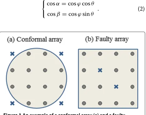
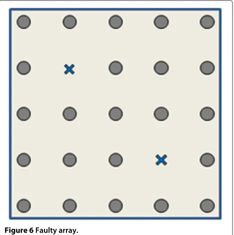
Although rectangular arrays, including uniform rectan-gular arrays (URA), are quite common in practical appli-cations, it is possible that the array is conformal to follow some prescribed shape or some of the elements fail to work, as illustrated in Figure 1, where the valid elements are denoted as circles in the area rounded up by the deep blue line while the blue ‘X’ denotes missing or faulty ele-ments (similarly hereinafter). So the array manifold is no longer rectangular, and it turns out to be a sub-array of the rectangular array.
In order to deal with irregular arrays mentioned above,
consider the rectangular array that consists of M× N
antenna elements in Equation 1. And it is assumed that there areDinvalid (missing or faulty) sensors indexed as
(md,nd), d = 1,· · ·,D, wheremd and nd are the row and column number of thedth invalid sensor, correspond-ingly. The location of all invalid sensors is supposed to be knowna prioriin this paper.
2.2 Representation of 2D DOA
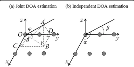
Most existing 2D DOA algorithms try to estimate
the azimuth and elevation angle (θ,ϕ), which is
(∠BOC,∠AOB) in Figure 2a. However, we consider
another definition of 2D DOA [16] in this paper, as given in Figure 2b or(∠AOC,∠AOD) in Figure 2a, where the purpose of direction finding is to estimate the two angles
(α,β)between the incoming signal andx-axis or y-axis, respectively. It is assumed that the signals come from above the antenna, as shown in Figure 2. Since OC⊥BC
andOC⊥AB, then we haveOC⊥AC. As a result,OC = OA·cosα = OB·cosθ = OA·cosϕcosθ. Similarly,
OD=OA·cosβ =OB·sinθ =OA·cosϕsinθ. Therefore, there exists a correspondence between(θ,ϕ)and(α,β):
cosα=cosϕcosθ
cosβ=cosϕsinθ . (2)
Figure 2Joint (a) and independent (b) 2D DOA estimation.
In this paper, we focus on the narrowband DOA estimation problem and the noise signals are assumed to be Gaussian additive noises. The incoming signals can be correlated or even coherent with each other. Using the narrowband model, we get the digital vector y(k) = y1(k),· · ·,yMN−D(k)
T
∈ C(MN−D)×1of com-plex amplitudes of the sensors at time instantkbellow (the superscript T denotes the transpose operation):
y(k)=As(k)+n(k), (3)
where it is assumed that there are P narrowband
far-field signals s(k) = [s1(k),· · ·,sP(k)]T ∈ CP×1. n(k) = [n1(k),· · ·,nMN−D(k)]T ∈ C(MN−D)×1 is the noise vector and A = [a(α1,β1),· · ·,a(αP,βP)] = [a(θ1,ϕ1),· · ·,a(θP,ϕP)]∈C(MN−D)×Pis the array man-ifold matrix whose columns are comprised ofPmanifold vectors. According to Equation 2, the element corre-sponding to a valid sensor at themth row andnth column in the manifold vectoraαp,βp
where the exponential term is written as the sum of factors related toαandβ, respectively, hence the two parameters to be estimated can be decoupled from each other.
If there are no invalid elements, the complex amplitudes of sensors are y(k) =[y1,1(k),· · ·,yM,1
According to (4), the manifold vector can be rewritten as the Kronecker product of two vectors:
aαp,βp
∈N×1denote the steering vectors of the linear sub-arrays that lie on thex-axis andy-axis, respectively. The super-scriptLdenotes ‘linear’. Thus, we can rewrite the signals received at the array in a decoupled form:
Y(k)=ALX(k)+N(k), (7) denotes manifold matrix whose columns are comprised of
Pmanifold vectors of the linear sub-array on thex-axis,
X(k) = different from each other, it is possible that some of
the incoming sources have the same α and there exist
multiple identical columns in the manifold matrix AL. Therefore, in order to make sure that all columns in the manifold matrix AL are different from each other, the 2D DOA of incoming sources can be denoted as
ingly, the incoming signals are denoted as s(k) =
s1,1(k),· · ·,s1,f1(k),· · ·,sP,1(k),· · ·,sP,fP(k)
T
∈CP0×1. Therefore, the signal matrixX(k)in Equation 7 becomes
From Equation 7, it can be observed that the informa-tion ofαandβis in the column and row spaces ofY(k), respectively. The manifold matrixALis decided byαand is not related toβ, while the signal matrixX(k)is deter-mined by β. Equation 7 can also be explained in terms of the rectangular manifold. Alpha can be estimated by analyzing the samples of the sub-array that lies on thex -axis and consists of sensors at(xm,y1)
,m = 1,· · ·,M. The linear sub-arrays that are parallel to x-axis in the rectangular array share the same manifold when only the estimation ofαis taken into account. Therefore, in order to estimateα, each snapshot received by the rectangular array can be regarded asNcorrelated snapshots of the lin-ear sub-array that lies on thex-axis. Then, 2D DOA can be estimated by solving two 1D DOA estimation problems successively instead of directly estimating 2D DOA. Since
αis decoupled fromβ, we can also estimateβfirstly and then estimateα. What is more, we will show in Section 3 that integrating the results of these two problems helps to improve the performance.
Now we still consider the rectangular array whose ele-ments are all valid and concentrate on the eleele-ments indexed(md,nd),d=1,· · ·,D. Obviously, we have:
which can be rewritten as:
Yf=ALX(k)+
In Equation 9, the received signals at the elements indexed (md,nd),d = 1,· · ·,Dare disregarded and set to zeros while the noise signals at these sensors change into nfmd,nd(k) = nmd,nd(k) − ymd,nd(k). The super-script f denotes ‘faulty.’ The case of faulty sensors can be processed in the above form. If there are D invalid elements, then no restriction is placed on the range of
ymd,nd(k),d=1,· · ·,Dsince there are no valid samples at these invalid sensors. As a result,nfmd,nd(k),d=1,· · ·,D in Equation 9 is unconstrained. In this way, the complex amplitudes of the sensors at a faulty rectangular array can still be written in the form of the decoupled signal model (Equation 9). However, it should be taken into account that the noise signals at the faulty sensors are uncon-strained and no longer distribute as noise signals at valid sensors. As a result, when the decoupled signal model is exploited, it should be noticed that the received signals at the faulty elements are set to be zero and the noise signals at these faulty elements are totally unknown and do not provide any additional information.
3 Proposed algorithm
Based on the above decoupled model, 2D DOA estimation can be achieved by two steps. Firstly, solve a 1D direction finding problem to estimate the first parameterαand get the information about the second parameterβ. This pro-cess can be accomplished by 1D DOA estimator directly working on the input data instead of using the covariance estimator, and information about the second parameter (signal matrix in Equation 7) can be obtained as well. Sec-ondly, solve another several 1D direction finding problems to estimateβbased on the rows extracted from the signal matrix and the correspondingαcan be obtained from the row number.
DOA estimation methods based on SSR have been found to have several advantages over conventional direc-tion finding methods and many of them work directly on the input data. Here, we pickl1-SVD [7] as our 1D DOA estimation algorithm and propose a new 2D DOA estima-tion method called 2D-l1-SVD. Exploiting the decoupled signal model, 2D-l1-SVD has a much lower computational load thanl1-SVD due to the successive estimation of 2D DOA parameters. Moreover, an improved version called enhanced-2D-l1-SVD is also proposed in this section to deal with multiple sources that are close to each other in
paper. On the other hand, it is obvious that JLZA-DOA [8] and the other sparse reconstruction based methods that work directly on the input data can also be extended to 2D situation using the aforementioned decoupled signal model similarly.
3.1 2D-l1-SVD algorithm
The steps of the 2D-l1-SVD algorithm are illustrated in Figure 3.
The notations that are used in this section are given in Table 1. For each notation, the superscript denotes the description of the variable and the subscript denotes the index of the variable.
Step1: Exploiting the decoupled signal model
The multiple snapshots received at the antenna
array can be denoted as a MN × T data matrix
Yant = yant(1),· · ·,yant(T) ∈ CMN×T where T
is the number of the snapshots. Here, yant(k) =
yant1,1(k),· · ·,yant1,N(k),· · ·,yantM,1(k),· · ·,yantM,N(k)T ∈
CMN×1 denotes the signal sampled at time instant k
(1 ≤ k ≤ T). The superscript ant denotes ‘antenna.’ According to the narrowband signal model, we have:
Yant=AS+Nant, (10)
whereA=aα1,β1,1
,· · ·,aα1,β1,f1
,· · ·,aαP,βP,1
, · · ·,aαP,βP,fP
∈ CMN×P0 is the manifold matrix of P0 incoming signals, S = [s(1),· · ·,s(T)] ∈ CP0×T is the signal matrix of the incoming signals and Nant = nant(1),· · ·,nant(T) ∈ CMN×T is the noise-signal matrix at the sensor array. Here,s(k)=[s1,1(k),· · ·, s1,f1(k),· · ·,sP,1(k),· · ·,sP,fP(k)]T∈ CP0×1 and nant
(k)=[n1,1ant(k),· · ·,n1,antN(k),· · ·,nantM,1(k),· · ·,nMant,N(k)]T∈
CMN×1denote the incoming signals and the noise signals sampled at time instantk(1 ≤ k ≤ T), respectively. As
mentioned before, faulty arrays can be treated in a sim-ilar way as a complete rectangular array. For rectangular arrays with faulty or missing elements, the manifold vec-tora(αp,βp,i)(1≤i≤fp) refers to the manifold vector of the complete rectangular array and the data matrixYant satisfiesymd,nd(k) =0,d= 1,· · ·,D,k =1,· · ·,T. Also, it should be noticed that noise signals at the faulty sensors
nmd,nd(k)are unconstrained.
For practical direction finding problems, we use the SVD of the data matrix to reduce both the computa-tional complexity and the sensitivity to noise, just like
l1-SVD [7]. The SVD of the data matrix isYant=UVH, where the superscript H denotes the conjugate transpose operation. Therefore, the data matrix is decomposed into the signal and noise subspaces. Then, the signal subspace that contains most of the signal power is kept
to reduce the dimension. Let DK =
IK,0K×(T−K)T
where IK is a K ×K identity matrix. Here, K denotes
the assumed number of sources and does not need
to be equal to the actual number of sources P0. And
it is indicated in [7] that l1-SVD maintains robust-ness to the assumed number of sources. Then, let Ysg = YantV DK =
ysg(1),· · ·,ysg(K) ∈ CMN×K, Ssg = SV DK = [ssg(1),· · ·,ssg(K)] ∈ CP0×K and Nsg=NantV DK =[nsg(1),· · ·,nsg(K)]∈CMN×Kwhere the superscript sg denotes ‘signal’. More specifically, ysg(k)=ysg1,1(k),· · ·,ysg1,N(k),· · ·,ysgM,1(k),· · ·,ysgM,N(k)T ∈CMN×1,ssg(k)=ssg
1,1(k),· · ·,s sg
1,f1(k),· · ·,s sg
P,1(k),· · ·, ssgP,f
P(k)
T
∈ CP0×1 and nsg(k) = nsg
1,1(k),· · ·, n sg 1,N
(k),· · ·,nsgM,1(k),· · ·,nsgM,N(k)T∈CMN×1. Therefore: Ysg=ASsg+Nsg. (11)
The manifold vector of the rectangular array can be rewritten as Kronecker product of two manifold vectors
Table 1 Notations used in section 3.1
Notation Size Definition
MN 1×1 The number of all the elements in the
rectangular array
D 1×1 The number of faulty elements in the
rectangular array
P0 1×1 The number of incoming sources
P 1×1 The number of differentα
T 1×1 The number of snapshots
K 1×1 The assumed number of incoming
sources
Yant MN×T The data matrix received at the array A MN×P0 The manifold matrix of the rectangular
array
S P0×T The signal matrix of incoming sources Nant MN×T The noise-signal matrix at the array
Ysg MN×K The reduced matrix containing most of the signal power
Ssg P0×K The reduced signal matrix Nsg MN×K The reduced noise signal matrix
Y M×NK The rearrangement ofYsg
AL M×P The manifold matrix of the linear sub-array onx-axis
X P×NK The signal matrix in the decoupled
model
N M×NK The rearrangement ofNsg
˜
AL M×Kα The dictionary of manifold vector of the linear sub-array onx-axis
˜
X Kα×NK The sparse signal matrix in the SSR in the αdomain
˜
BL N×Kβ The dictionary of manifold vector of the linear sub-array ony-axis
˜
(see Equation 6). Then, expressing the equation above in a matrix form similarly as Equation 7, we have: matrix of the linear sub-array on thex-axis and no longer
depends on β-DOA while the information ofβ-DOA is
now contained in the signal matrixX. And:
Yk =
Step 2: Estimate α from multiple measurement vectors
(MMV)
An overcomplete representation of AL in terms of all possibleα, which is denoted asA˜L, is introduced here. Let
˜
α1,· · ·,α˜Kα
be a sampling grid of all directions of inter-est in theαdomain. The number of potential directions in theαdomainKαis typically much greater than the num-ber of differentα, i.e.,Kα P. Then,A˜Lis composed of steering vectors corresponding to each potentialα as its columns. Here, the steering vectors inA˜Lcorrespond to the linear sub-array on thex-axis. Therefore, Equation 12 can be rewritten in a sparse reconstruction form:
Y =A˜LX˜ +N, (14)
elements, estimation ofαcan be accomplished by solving
a MMV problem based onl1-norm minimization:
min
where thel1-term enforces sparsity of the representation.
˜ the above MMV problem. Then, the pseudo spectrum of
αis obtained by calculating thel2-norm of each row in the signal matrixXˆ, i.e., the amplitude of the pseudo spectrum atα˜kα isxˆkα2.
In the MMV problems based onl1-norm minimization
mentioned above,l1-term enforces sparsity whilel2-term forces the residual to be small. The residual specifies how much noise we wish to allow. For rectangular arrays with invalid elements, the noise signals or residuals of invalid elements are unknown while the residuals of valid ele-ments are forced to be small. Hence, the constrained condition of the l2-term should be revised, taking into consideration of invalid elements. On the other hand, the spatial sparsity still exists, sol1-term remains unchanged. When there are invalid elements, the columns ofY in the above MMV problem can be regarded as multiple snapshots of a linear subarray, in which there exists invalid data. Residual at these invalid elements should be uncon-strained since no information of these elements is known
a priori. LetNres= Y −A˜LX˜ ∈CM×NK. Therefore,
esti-mation ofα can be accomplished by solving a modified
MMV problem based onl1-norm minimization:
min
where thel1-term enforces sparsity of the representation. We will specify the sufficient condition of correct recov-ery of the signal matrixXˆ in Section 4. Then, the pseudo spectrum ofα is obtained by calculating thel2 norm of each row in the signal matrixXˆ similarly.
Just like [7], with the knowledge of the distribution of noise, we can find a confidence interval forN2F, then use its upper value forσ12.
Step3: Estimateβbased on the signal matrix
Let P denote the number of different α of the
sources. Then, the pseudo spectrum of α may have
P local maxima which are denoted as αˆ1,· · ·,αˆP
.
The row number in the signal matrix Xˆ that
corre-sponds to these local maxima is denoted as{i1,· · ·,iP}.
The rows of Xˆ corresponding to possible α
con-tain information about β. Let the ith row of Xˆ be
. Similarly, an overcomplete representation ofBLp
is introduced. LetB˜L = (1≤p≤P). Taking into consideration of the noises intro-duced in the above MMV problems, we can solve another
PMMV problems to estimateβ:
min
estimation ofβis accomplished.
Although the distribution of the elements inXˆiis diffi-cult to estimate,σ22can be determined by the upper value ofKnsgm1(k),· · ·,nsgmN(k)22empirically.
Step4: Calculate(θ,ϕ)based on(α,β)if needed. The effects of invalid elements on the degree of freedom will be studied in Section 4.
3.2 Enhanced 2D-l1-SVD algorithm
We will show in Section 5 that 2D-l1-SVD works prop-erly when the sources are well separated in both α and
β domains. As illustrated in [14], there exists a source of bias inherent in the nature of the sparsity enforcing functionals. For example, consider a 1D case:
X=AS+N, (20) potentialθ.a(θ)is the steering vector of a linear array. It is assumed that there are only two sources, which are from
θ1 andθ2, impinging on the linear array. Obviously, the sparsity condition is satisfied with proper
˜
θ1,· · ·,θ˜Kθ
two sources are too close to each other although the sparsity condition is still satisfied [14].
The problem still exists when l1-SVD is extended to 2D cases. If two sources, which are from (α1,β1) and (α2,β2), are close to each other in bothα andβ domains soa(α1,β1)is quite similar toa(α2,β2), thenl1-SVD will get biased results. However, l1-SVD can work properly and get nearly unbiased results when distinguished sig-nals are close to each other inαdomain but well separated to each other inβ domain while 2D-l1-SVD gets biased results in theαdomain. An enhanced 2D-l1-SVD is pro-posed to solve this problem, and it still has a much lower complexity thanl1-SVD.
We demonstrate the problem of the primary 2D-l1
-SVD algorithm with an example and then illustrate the main idea of the enhanced-2D-l1-SVD. As illustrated in Figure 4a,b, there are five sources impinging on the array. The true DOAs of these five sources are αp,βp
, p =
1,· · ·, 5. Andα1 ≈ α2,α4 ≈ α5,β1 ≈ β5, andβ2 ≈ β4. Using 2D-l1-SVD, we estimateαfirstly and then estimate β(denoted as 2D-l1-SVD-α), as shown in Figure 4a. Since α1 is very close to α2, they cannot be identified from each other in α domain.α4 andα5cannot be identified either. As a result, only three estimates,αˆ1≈(α1+α2) /2,
ˆ
α2 ≈ α3, andαˆ3 ≈ (α4+α5) /2, are obtained by solv-ing a MMV problem due to the signals gathersolv-ing in theα domain. Then, another three MMV problems are solved to get the estimates in theβdomain. For example, we can
extract the row information that corresponds toαˆ1from the signal matrixXˆ and get two estimates,βˆ1,1andβˆ1,2. So the estimates of DOAs of sources 1 and 2 are(αˆ1,βˆ1,2) and (αˆ1,βˆ1,1), as illustrated in Figure 4a. Similarly, the estimates of the DOAs of sources 3 to 5 are (αˆ2,βˆ2,1), (αˆ3,βˆ3,1), and(αˆ3,βˆ3,2). Apparently, the estimation of the DOAs of sources 1, 2, 4, and 5 inα domain is not accu-rate. If we estimateβ firstly and then estimateα(denoted as 2D-l1-SVD-β), there is a similar problem sinceβ1≈β5 andβ2 ≈ β4, as shown in Figure 4b. And the estimates of the DOAs of sources 1 to 5 using 2D-l1-SVD-β are denoted as (αˆ3,1,βˆ3), (αˆ1,1,βˆ1), (αˆ2,1,βˆ2), (αˆ1,2,βˆ1), and (αˆ3,2,βˆ3), respectively. However, these sources can be dis-tinguished from each other usingl1-SVD since the DOAs of the sources are well separated either inαdomain orβ domain.
Although 2D-l1-SVD-α cannot accurately estimate α when there exist multiple sources close to each other inα domain, it can provide preciseβ-DOA if the sources are not too close to each other inβdomain since the informa-tion ofβis in the column of the input data matrix. Similar results can be obtained ifβis firstly estimated using 2D-l1 -SVD-β. So the enhanced algorithm is designed to combine the estimation results in conjunction with a selection strategy.
The selection strategy is based on the condition that any two sources are not too close to each other in bothαandβ domains. The main idea is to make pairs of the estimation
Table 2 Arithmetic complexity of 2D-l1-SVD andl1-SVD β corresponds to the same source. In Figure 4a, sources 1 and 2 are close to each other in α domain, so αˆ1 is inaccurate whileβˆ1,2 andβˆ1,1 are precise. In Figure 4b, we get three different β, in which βˆ3 is closest to βˆ1,2 and βˆ1 is closest to βˆ1,1. Consider the estimation of α corresponding toβˆ3 and we find that αˆ3,1 is the closest to αˆ1. Therefore,(αˆ1,βˆ1,2) and (αˆ3,1,βˆ3) are considered to be a pair. Similarly, we have the other four pairs. For pairs corresponding to sources 1, 2, 4, and 5, 2D-l1 -SVD-αhas got more precise estimation ofβand 2D-l1-SVD-β has got more precise estimation ofα. Therefore, primary results of 2D-l1-SVD-α and 2D-l1-SVD-β are corrected, as illustrated in Figure 4c. It should be noticed that the pairing process in enhanced-2D-l1-SVD is quite different from the pair-matching in [16]. Given the set of eleva-tion angles and azimuth angles, which is{θ1,· · ·,θP}and {ϕ1,· · ·,ϕP}, respectively, the conventional pair-matching process in [16] choose P final estimates from P2 possi-ble pairs by making use of the statistical analysis of the received data. In enhanced-2D-l1-SVD, final DOA esti-mates are extracted from two existed set of 2D DOA without using information of the received data.
Another issue that needs to be taken into account is that spurious peaks may appear in the pseudo spectrum ofl1 -SVD due to inappropriate regularization parameter but the selection strategy in enhanced-2D-l1-SVD provides a detection of spurious peaks. For a certain(αˆi,βˆi) got by 2D-l1-SVD-α, a corresponding(αˆj,βˆj)got by 2D-l1 -SVD-βcan be found to make a pair with(αˆi,βˆi). Then,(αˆi,βˆi) is considered to be a false peak if:
αˆi− ˆαj2
+βˆi− ˆβj 2
> δ, (21)
whereδis a threshold and the beamwidth of the array pat-tern is a reasonable choice forδ. The overall procedure of the enhanced 2D-l1-SVD is summarized as follows:
Step 1: Complete the 2D-l1-SVD-α.
Estimateαfirstly and then estimateβ. There are Pdifferentαand the estimation results are denoted asα= {(αˆ1,βˆ1,1),· · ·,(αˆ1,βˆ1,f1),· · ·, (αˆP,βˆP,1),· · ·,(αˆP,βˆP,fP)}. Forαˆp, there arefp
differentβ.
Step 2: Complete the 2D-l1-SVD-β.
Estimateβfirstly and then estimateα. There are Qdifferentβand the estimation results are denoted asβ = {(αˆ1,1,βˆ1),· · ·,(αˆ1,g1,βˆ1),· · ·, was considered to be a false peak. If
Using l1-SVD as 1D DOA estimators during successive
estimation, 2D-l1-SVD has several advantages over con-ventional 2D methods, including high resolution, robust-ness to the number of snapshots, low SNR, and coherent sources due to the use of sparse reconstruction [7]. In this section, we compare the performance of 2D-l1-SVD andl1-SVD and study about the effect of invalid elements. Firstly, we demonstrate that the computational complex-ity of 2D-l1-SVD is much lower than that of l1-SVD. Secondly, we study about the degree of freedom of
2D-l1-SVD. Then, we will show that 2D-l1-SVD keeps better robustness over the assumed number of sources in the
Table 4 Time cost of different methods
Time (s) Kαβ
46 91 181 361
2D-MUSIC 0.3315 1.2961 5.1043 20.2029
l1-SVD 2.7922 12.9736 59.9812 397.105
2D-l1-SVD 0.4381 0.4929 0.5964 0.8356
Enhanced-2D-l1-SVD 1.0704 1.4574 1.6928 2.5747
presence of multiple sources. And finally, we investigate the number of sources that 2D-l1-SVD can process with both rectangular arrays and faulty rectangular arrays.
4.1 Computational complexity
Sparse reconstruction methods based on l1-norm
minimization can be achieved by second-order cone
programming (SOCP). For optimizing the joint
opti-mization problem over K vectors in SOCP framework
using an interior point method, the arithmetic complex-ity is OK3K3
θ
, where Kθ is the number of potential
directions [7,19]. Therefore, we have the computa-tional load of 2D-l1-SVD and l1-SVD in Table 2. Since Kα and Kβ are always much bigger than M,N,K, the
arithmetic cost of 2D-l1-SVD is much smaller than
l1-SVD.
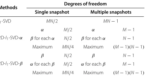
4.2 Degrees of freedom
A necessary and sufficient condition [20] from the mea-surementsX=AS,|supp(S)| =k, to uniquely determine Sis (|supp(S)|denotes the union over all the individual supports∪isupp(si)forS=[s1,· · ·,sl]):
|supp(S)|< (spark(A)−1+rank(X)) /2, (22)
where the spark ofA is defined as the smallest number
of columns in A that are linearly dependent. For DOA
estimation problems, the measurement matrix X and
the signal matrixSstand for the sampled snapshots at the array and the incoming source signals, respectively. The dictionaryAis a matrix composed of the steering vectors corresponding to each potential DOA as its columns. And the number of columns inAis much bigger than the num-ber of rows inA. Let L0 denote the number of sensors in the array. For linear or rectangular arrays whose mani-fold matrix is similar to a Vandermonde matrix, spark(A) is equal to L0+ 1 if the potential DOAs in the dictio-nary are not too close to each other so that the mutual coherence [20] is small. On the hand, rank(X) = 1 if the number of snapshots is only one and rank(X) =K if the number of singular vectors used is sufficient, e.g., equal to the number of sources. So empirically, thel1-SVD tech-nique can resolveM−1 sources with anM-sensors array if they are not located too close to each other [7]. This holds under the assumption that the number of singular vectors used inl1-SVD is sufficient, e.g., equal to the number of sources. When fewer singular vectors are taken than the number of sources, the number of resolvable sources may decrease.
For aM×Nrectangular array, with no consideration of array ambiguity and only one snapshot available,l1-SVD can process up toMN/2 sources. For 2D-l1-SVD-α, there exists a coherence between the samples of sub-arrays at different columns of the array as far as the estimation of
αis concerned, so 2D-l1-SVD-α can processM/2 differ-entα and up toN/2 differentβ for eachα. When there are enough snapshots and the number of uncorrelated columns in the data matrixX is not less than the num-ber of sensors,l1-SVD can process up toMN−1 sources, while 2D-l1-SVD-αcan process up toM−1 differentαand N−1 differentβfor each certainα. Similarly, 2D-l1 -SVD-β can process up toN/2 different β andM/2 different
αwith only one snapshot. When there are enough
snap-shots, 2D-l1-SVD-β can process up toN−1 differentβ andM−1 differentα. So the number of sources that
2D-l1-SVD or enhanced-2D-l1-SVD can process is less than l1-SVD when the sources are well separated in bothαand βdomains. However, when the sources are gathering inα orβ domains and several sources may be treated as one group in successive parameter estimation,
enhanced-2D-l1-SVD can resolve up to(M−1)(N−1)sources, which is close to l1-SVD if M and N are sufficiently large in practical application. The degrees of freedom of different methods are illustrated in Table 3.
4.3 The assumed number of sources
The l1-SVD technique works on the K singular vectors
whereK is the assumed number of sources. It has been
illustrated in [7] thatl1-SVD has a low sensitivity toK.
In [7], it is illustrated that l1-SVD can resolve
M − 1 sources using an M-sensor array. However,
when fewer singular vectors are taken than the num-ber of sources, the condition in (22) may be not satisfied and the number of resolvable sources may decrease. This limitation still exists in 2D situation. Assume that the 2D DOA of incoming sources are {(α1,β1,1),· · ·,(α1,β1,f1),· · ·,(αP,βP,1),· · ·,(αP,βP,fP)},
andP0 = P p=1
fp. To resolveP0sources that haveP
differ-entα, the assumed number of sources forl1-SVD should be not less thanP0ifP0is sufficiently large (for example, P0is close to the number of sensors). The number of sin-gular vectors should not be less thanPorfpto resolveP differentαandfpdifferentβ, correspondingly. As a result, if the assumed number of sources for 2D-l1-SVD is not less than max{P,f1,· · ·,fP}, the 2D-l1-SVD can resolveP0 sources. So 2D-l1-SVD may resolve more sources with fewer singular vectors. Moreover, 2D-l1-SVD may have an even smaller computational complexity by taking a smaller number of singular vectors.
4.4 Faulty or nonrectangular arrays
When there are only a small number of elements with failure in the array, the faulty elements have little effect on the performance of 2D-l1-SVD. The faulty array is no longer rectangular while it can be regarded as a rectangu-lar array with missing elements. Under this circumstance, the degree of freedom may be affected while 2D-l1-SVD is still able to produce correct DOA estimates. Empirically, 2D-l1-SVD-αcan resolveM0−1 differentαandN0−1 differentβfor eachαwhen the sources are not too close to
Figure 7Pseudo spectrum.(a)αin 2D-l1-SVD-α.(b)βfor two differentαin 2D-l1-SVD-α.(c)βin 2D-l1-SVD-β.(d)αfor two differentβin 2D-l1-SVD-β.
Figure 9Bias inαandβdomain of 2D-l1-SVD andl1-SVD in localizing two sources as a function of the source separation.
each other. Here,M0andN0denote the minimum number of valid elements in each row or column of the rectangu-lar array. On the other hand, there should not be too many invalid elements, or the distances between valid elements become so large that there will be grating lobes.
5 Simulation results
In this section, several simulations are conducted to val-idate the advantages of 2D-l1-SVD. All simulations are
performed using MATLAB 2012a running on an Intel Core i7 3770 CPU @ 3.4 GHz with 16 GB RAM, under Windows 7.
5.1 Time cost
Firstly, we compare the computation time of 2D-MUSIC,
l1-SVD, 2D-l1-SVD, and enhanced 2D-l1-SVD. Consider
a 5 × 5 URA with sensors spaced half a wavelength
apart and there are three uncorrelated sources with 100
snapshots. The DOAs of the three sources are (120°, 70°), (80°, 50°), and (50°, 130°). And SNR = 10 dB. The time that the four methods cost against Kαβ, which repre-sents the density of the grids or the number of potential source locations (the grids or potential locations are set as 0,π/Kαβ−1,· · ·,Kαβ −2π/Kαβ−1,π for bothαandβ domains), is demonstrated in Table 4. Each value in the table is an average over 50 trials. Table 4 shows that 2D-l1-SVD and enhanced 2D-l1-SVD have a much lower computational load than other methods. The cost time of enhanced 2D-l1-SVD is nearly twice of that of 2D-l1-SVD, and it is affected by the number of differentα andβ.
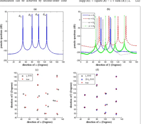
5.2 Pseudo spectrum with multiple sources
The pseudo spectrum of 2D-l1-SVD and l1-SVD when
there are 13 independent sources (four different α)
impinging on the 5×5 URA with sensors spaced half a
wavelength apart is illustrated in Figure 5. The true DOAs are (50°, 65°), (50°, 95°), (80°, 60°), (80°, 90°), (80°, 120°), (80°, 145°), (100°, 50°), (100°, 70°), (100°, 100°), (127°, 50°), (127°, 80°), (127°, 110°), and (127°, 140°). SNR = 10 dB, and there are 100 snapshots. 2D-l1-SVD is able to identify
four different α and give correct DOA estimation when
the assumed number of sources isK = 3 (Figure 5a,b,d).
l1-SVD has given correct estimation ifK=13 (Figure 5d)
while there are spurious peaks in the spectrum ofl1-SVD ifK = 3 (Figure 5c). So 2D-l1-SVD may perform better with fewer singular vectors.
5.3 Bias
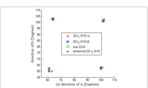
Many DOA estimation methods may have difficulty resolving closely spaced sources, and there is bias inherent in the nature of sparsity enforcing functionals [14]. Con-sider the faulty array in Figure 6 with sensors spaced half a wavelength apart. There are four uncorrelated sources with a SNR = 10 dB. And there are 100 snapshots. The pseudo spectrum of 2D-l1-SVD-αand 2D-l1-SVD-βwhen the true DOAs are (61°, 60°), (64°, 103°), (100°, 63°), and (102°, 101°) is illustrated in Figure 7. We can see that the peaks of the spectrum in Figure 7a,c are biased. A final estimation of DOA is given in Figure 8 by combining the results got by 2D-l1-SVD-α and 2D-l1-SVD-β, and the results are correct.
The bias of the DOA estimation of two sources with different angular separation between them is investigated here. Consider the faulty array in Figure 6. The source 1 is held fixed at (62.6°, 58.7°) and the source 2 is moving from the location of source 1 linearly. And SNR = 10 dB. Bias in theαorβdomain of 2D-l1-SVD andl1-SVD as a func-tion of the source separafunc-tionδ0(degrees) is demonstrated in Figure 9 while source 2 is located at (62.6° +δ0, 58.7° +
δ0). The values on each curve are an average over 50 tri-als. Figure 9 shows the presence of bias for low separations using both enhanced-2D-l1-SVD andl1-SVD, and the bias disappears whenδ0>20° for both algorithms.
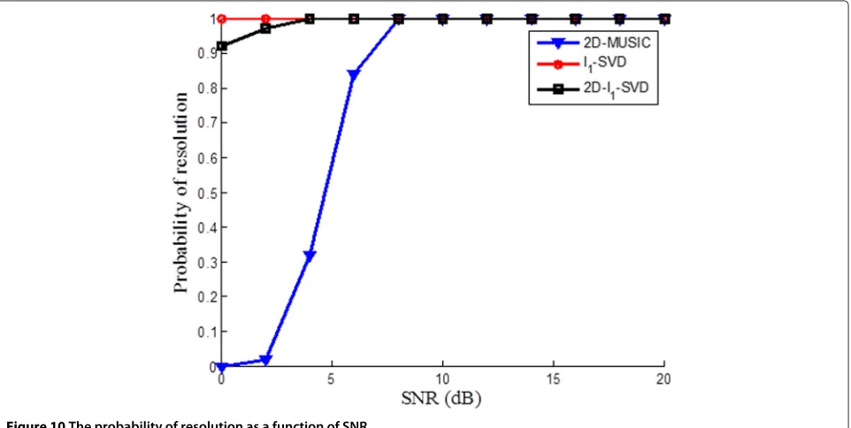
5.4 Resolution capability
The resolution performance of the proposed algorithms and the 2D-MUSIC algorithm is compared here. Con-sider the faulty array in Figure 6. There are two incoming sources from (80.3°, 106.4°) and (85.3°, 111.4°). There are 100 snapshots. The probability of resolution [21] as a func-tion of SNR is illustrated in the Figure 10, and it is based on 100 trials. We can see that bothl1-SVD and 2D-l1-SVD outperform 2D-MUSIC when the SNR is less than 8 dB. And 2D-l1-SVD performs close tol1-SVD. Note that the resolution probability of enhanced-2D-l1-SVD is the same to that of 2D-l1-SVD since the results of the enhanced algorithm are based on the estimates of 2D-l1-SVD.
5.5 RMSE
The root mean squared error (RMSE) is defined as
RMSE= 1
Consider the faulty array in Figure 6. The RMSE of dif-ferent methods against SNR based on 100 realizations compared with the Cramer-Rao lower bound (CRLB) [22] when there are a single source from (80.3°, 106.4°) with 100 snapshots is given in Figure 11a. And the RMSE against the number of snapshots when SNR of the single source is 5 dB is given in Figure 11b. It shows that 2D-MUSIC, 2D-l1-SVD, and enhanced-2D-l1-SVD perform close to the CRLB when there is only one source. The RMSE as a function of SNR based on 100 realizations when there are two uncorrelated sources from (80.3°, 106.4°) and (100.9°, 127.1°) is given in Figure 11c, and the RMSE against the number of snapshots when SNR of the two sources is 5 dB is given in Figure 11d. We can see that the performance of 2D-MUSIC deteriorates when there are not enough snap-shots (less than twice of the number of antennas) while SSR based algorithms work properly.
6 Conclusions
In this paper, a new 2D estimation method called
2D-l1-SVD and its improved version enhanced-2D-l1-SVD
are proposed for rectangular arrays. They are proved to be able to work for rectangular arrays even with miss-ing or faulty elements. Theoretical analysis and simulation results indicate that 2D-l1-SVD has a much lower arith-metic complexity due to successive parameter estimation while performing close to the popular l1-SVD. What is more, 2D-l1-SVD has better robustness to the assumed number of sources and enhanced-2D-l1-SVD is able to detect spurious peaks which are caused by inappropriate regularization parameter.
Competing interests
The authors declare that they have no competing interests.
Acknowledgements
The authors would like to thank the anonymous reviewers for their valuable comments that improved the manuscript.
Received: 26 August 2014 Accepted: 17 January 2015
References
1. H Krim, M Viberg, Two decades of array signal processing research: the parametric approach. IEEE Signal Process. Mag.13(4), 67–94 (1996) 2. E Tuncer, B Friedlander,Classical and Modern Direction-of-Arrival
Estimation(Elsevier Academic Press, Burlington, USA, 2009)
3. J Capon, High-resolution frequency-wavenumber spectrum analysis. Proc IEEE.57(8), 1408–1418 (1969)
4. R Schmidt, Multiple emitter location and signal parameter estimation. IEEE Trans. Antennas Propag.34(3), 276–280 (1986)
5. R Roy, T Kailath, ESPRIT-estimation of signal parameters via rotational invariance techniques. IEEE Trans. Acoustics Speech Signal. Process.37(7), 984–995 (1989)
6. P Stoica, K Sharman, Maximum likelihood methods for direction-of-arrival estimation. IEEE Trans. Acoustics Speech Signal. Process.38(7), 1132–1143 (1990)
7. D Malioutov, M Cetin, A Willsky, A sparse signal reconstruction perspective for source localization with sensor arrays. IEEE Trans. Signal Process.53(8), 3010–3022 (2005)
8. M Hyder, K Mahata, Direction-of-arrival estimation using a mixedl2,0 norm approximation. IEEE Trans. Signal Process.58(9), 4646–4655 (2010) 9. P Stoica, P Babu, J Li, A sparse covariance-based estimation method for
array processing. IEEE Trans. Signal Process.59(2), 629–638 (2011) 10. J Zheng, M Kaveh, Sparse spatial spectral estimation: a covariance fitting
algorithm, performance and regularization. IEEE Trans. Signal Process. 61(11), 2767–2777 (2013)
11. X Xu, X Wei, Z Ye, DOA estimation based on sparse signal recovery utilizing weightedl1-norm penalty. IEEE Signal Process. Lett.19(3), 155–158 (2012) 12. A Gershman, M Rubsamen, M Pesavento, One-and two-dimensional
direction-of-arrival estimation: an overview of search-free techniques. Signal Process.90, 1338–1349 (2010)
13. Y Wang, L Lee, A tree structure one-dimensional based algorithm for estimating the two-dimensional direction of arrivals and its performance analysis. IEEE Trans. Antennas Propag.56(1), 178–188 (2008)
14. D Malioutov, A sparse signal reconstruction perspective for source localization with sensor arrays. PhD thesis, Massachusetts Institute of Technology (2003)
15. Y Liu, M Wu, S Wu, Fast OMP algorithm for 2D angle estimation in MIMO radar. Electronics Lett.46(6), 444–445 (2010)
16. S Kikuchi, H Tsuji, A Sano, Pair-matching method for estimating 2-D angle of arrival with a cross-correlation matrix. IEEE Antennas Wireless Propag. Lett.5(1), 35–40 (2006)
17. Q Liu, S OuYang, L Jin, Two-dimensional DOA estimation with L-shaped array based on a jointly sparse representation. Inf. Technol. J.12, 2037–2042 (2013)
19. M Lobo, L Vandenberghe, S Boyd, H Lebret, Applications of second-order cone programming. Linear Algebra Its Applicat. Special Issue Linear Algebra Control Signals Image Process.284, 193–228 (1998)
20. M Davies, Y Eldar, Rank awareness in joint sparse recovery. IEEE Trans. Inf. Theory.58(2), 1135–1146 (2012)
21. Q Zhang, Probability of resolution of the MUSIC algorithm. IEEE Trans. Signal Process.43(4), 978–987 (1995)
22. Y Hua, T Sarkar, A note on the Cramer-Rao bound for 2-D direction finding based on 2-D array. IEEE Trans. Signal Process.39(5), 1215–1218 (1991)
Submit your manuscript to a
journal and benefi t from:
7Convenient online submission 7Rigorous peer review
7Immediate publication on acceptance 7Open access: articles freely available online 7High visibility within the fi eld
7Retaining the copyright to your article