Novel pattern recognition approaches for transcriptomics data analysis

(1)

University of Windsor University of Windsor

Scholarship at UWindsor

Electronic Theses and Dissertations Theses, Dissertations, and Major Papers

2014

Novel pattern recognition approaches for transcriptomics data

analysis

Iman Rezaeian University of Windsor

Follow this and additional works at: https://scholar.uwindsor.ca/etd

Recommended Citation Recommended Citation

Rezaeian, Iman, "Novel pattern recognition approaches for transcriptomics data analysis" (2014). Electronic Theses and Dissertations. 5085.

https://scholar.uwindsor.ca/etd/5085

This online database contains the full-text of PhD dissertations and Masters’ theses of University of Windsor students from 1954 forward. These documents are made available for personal study and research purposes only, in accordance with the Canadian Copyright Act and the Creative Commons license—CC BY-NC-ND (Attribution, Non-Commercial, No Derivative Works). Under this license, works must always be attributed to the copyright holder (original author), cannot be used for any commercial purposes, and may not be altered. Any other use would require the permission of the copyright holder. Students may inquire about withdrawing their dissertation and/or thesis from this database. For additional inquiries, please contact the repository administrator via email

(2)

NOVEL PATTERN RECOGNITION APPROACHES FOR

TRANSCRIPTOMICS DATA ANALYSIS

by

Iman Rezaeian

A Dissertation

Submitted to the Faculty of Graduate Studies through School of Computer Science in Partial Fulfillment of the Requirements for

the Degree of Doctor of Philosophy at the University of Windsor

Windsor, Ontario, Canada 2014

c

(3)

NOVEL PATTERN RECOGNITION APPROACHES FOR

TRANSCRIPTOMICS DATA ANALYSIS

by

IMAN REZAEIAN

APPROVED BY:

M. R. El-Sakka, External Examiner

Department of Computer Science, Western University

E. Abdel-Raheem

Department of Electrical and Computer Engineering

J. Lu

School of Computer Science

X. Yuan

School of Computer Science

A. Ngom, Co-Advisor School of Computer Science

L. Rueda, Advisor School of Computer Science

(4)

Declaration of Co-Authorship and

Previous Publication

I. Co-Authorship Declaration:

I hereby declare that this Dissertation incorporates the outcome of a joint research

un-dertaken in collaboration with Yifeng Li, Martin Crozier, Dr. Eran Andrechek, Dr. Alioune

Ngom, Dr. Luis Rueda and Dr. Lisa Porter. The collaboration is covered in Chapter 6 of

the Dissertation. In this research, experimental designs, applying and optimizing different

machine learning methods for prediction, numerical and visual analysis were performed by

the author.

I am aware of the University of Windsor Senate Policy on Authorship and I certify

that I have properly acknowledged the contribution of other researchers to my Dissertation,

and have obtained written permission from each of the co-author(s) to include the above

material(s) in my Dissertation. I certify that, with the above qualification, this Dissertation,

and the research to which it refers, is the product of my own work.

II. Declaration of Previous Publications:

This Dissertation includes 5 original papers that have been previously published/submitted

for publication in conferences and peer reviewed journals, as follows:

I certify that I have obtained a written permission from the copyright owner(s) to

(5)

iv

Dissertation chapter Publication title

Chapter 2 Luis Rueda, Iman Rezaeian: A Fully Automatic Gridding Method for

cDNA Microarray Images. BMC Bioinformatics (2011) 12: 113.

Chapter 3

Luis Rueda, Iman Rezaeian: Applications of Multilevel Thresholding Algorithms to Transcriptomics Data. Progress in Pattern Recognition, Image Analysis, Computer Vision, and Applications - 16th Iberoameri-can Congress (CIARP), Chile, 2011: 26-37.

Chapter 4

Iman Rezaeian, Luis Rueda: A new algorithm for finding enriched regions in ChIP-Seq data. ACM International Conference on Bioin-formatics, Computational Biology and Biomedicine (BCB), Chicago, USA, 2012: 282-288.

Chapter 5

Iman Rezaeian, Luis Rueda: CMT: A Constrained Multi-Level

Thresh-olding Approach for ChIP-Seq Data Analysis. PLoS ONE 9(4):

e93873, 2014.

Chapter 6

Iman Rezaeian, Yifeng Li, Martin Crozier, Eran Andrechek, Alioune Ngom, Luis Rueda, Lisa Porter: Identifying Informative Genes for Pre-diction of Breast Cancer Subtypes. Pattern Recognition in Bioinformat-ics - 8th IAPR International Conference (PRIB), France, 2013: 138-148.

clude the above published material(s) in my Dissertation. I certify that the above material

describes work completed during my registration as graduate student at the University of

Windsor.

I declare that, to the best of my knowledge, my Dissertation does not infringe upon

any-one copyright nor violate any proprietary rights and that any ideas, techniques, quotations,

or any other material from the work of other people included in my Dissertation, published

or otherwise, are fully acknowledged in accordance with the standard referencing

prac-tices. Furthermore, to the extent that I have included copyrighted material that surpasses

the bounds of fair dealing within the meaning of the Canada Copyright Act, I certify that I

have obtained a written permission from the copyright owner(s) to include such material(s)

(6)

v

revisions, as approved by my Dissertation committee and the Graduate Studies office, and

that this Dissertation has not been submitted for a higher degree to any other University or

(7)

Abstract

We proposed a family of methods for transcriptomics and genomics data analysis based

on multi-level thresholding approach, such as OMTG for sub-grid and spot detection in

DNA microarrays, and OMT for detecting significant regions based on next generation

sequencing data. Extensive experiments on real-life datasets and a comparison to other

methods show that the proposed methods perform these tasks fully automatically and with a

very high degree of accuracy. Moreover, unlike previous methods, the proposed approaches

can be used in various types of transcriptome analysis problems such as microarray image

gridding with different resolutions and spot sizes as well as finding the interacting regions

of DNA with a protein of interest using ChIP-Seq data without any need for parameter

adjustment. We also developed constrained multi-level thresholding (CMT), an algorithm

used to detect enriched regions on ChIP-Seq data with the ability of targeting regions within

a specific range. We show that CMT has higher accuracy in detecting enriched regions

(peaks) by objectively assessing its performance relative to other previously proposed peak

finders. This is shown by testing three algorithms on the well-known FoxA1 Data set, four

transcription factors (with a total of six antibodies) for Drosophila melanogaster and the

H3K4ac antibody dataset. Finally, we propose a tree-based approach that conducts gene

selection and builds a classifier simultaneously, in order to select the minimal number of

genes that would reliably predict a given breast cancer subtype. Our results support that this

(8)

vii

modified approach to gene selection yields a small subset of genes that can predict subtypes

with greater than 95% overall accuracy. In addition to providing a valuable list of targets for

diagnostic purposes, the gene ontologies of the selected genes suggest that these methods

have isolated a number of potential genes involved in breast cancer biology, etiology and

(9)

Dedication

to my love, Forough

(10)

Acknowledgements

I would like to take this opportunity to express my sincere gratitude to Dr. Luis Rueda, my

supervisor, for his steady encouragement, patient guidance and enlightening discussions

throughout my graduate studies. Without his help, the work presented here could not have

been possible.

I also want to express my gratitude to my co-advisor Dr. Alioune Ngom, who shared

many works with me and gave me many useful suggestions during my research.

I also wish to express my appreciation to Dr. Mahmoud R. El-Sakka, Western

Univer-sity, Dr. Esam Abdel-Raheem, Department of Electrical and Computer Engineering, Dr.

Jianguo Lu and Dr. Xiaobu Yuan, School of Computer Science for being in the committee

and spending their valuable time. Moreover, I would like to express my gratitude to Dr.

Lisa porter for her constructive suggestions and feedbacks.

Finally, I would like to thank all of my colleagues in pattern recognition and

bioinfor-matics lab, especially, Forough Firoozbakht, Mina Maleki and Yifeng Li for their consistent

support and help.

(11)

List of Figures

1.1 (a) Original DNA microarray image, 20391-ch1 (green channel), from the

SMD; (b) sub-grid extracted from the 8th column and 3rd row. . . 4

1.2 Diagrammatic view of the work flow of ChIP-Seq data analysis. . . 7

2.1 Sub-grid and spot detection in one of the SMD dataset images. Detected

sub-grids in AT-20387-ch2 (left), and detected spots in one of the sub-grids

(right). . . 30

2.2 Sub-grid and spot detection in one of the GEO dataset images. Detected

grids in GSM16101-ch1 (left), and detected spots in one of the

sub-grids (right). . . 31

2.3 Sub-grid and spot detection in one of the DILN dataset images. Detected

sub-grids in Diln4-3.3942B (left) and detected spots in one of the sub-grids

(right). . . 32

2.4 Failure to detect some spot regions due to the extremely contaminated

im-ages with artifacts in the sub-grid located in the first row and fourth column

of AT-20392-ch1 from the SMD dataset. . . 33

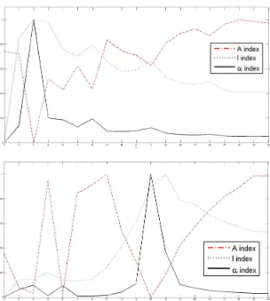
2.5 Plots of the index functions for AT-20387-ch2: (top) the values of the I, A

andαindices for horizontal separating lines, and (bottom) the values of the

I, A andαindices for vertical separating lines. . . 34

(16)

LIST OF FIGURES xv

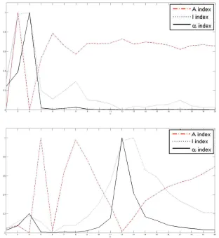
2.6 Plots of the index functions for the GSM16101-ch1: (top) the values of the

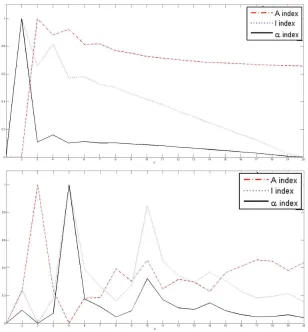
I, A andα indices for horizontal separating lines, and (bottom) the values of the I, A andαindices for vertical separating lines. . . 35 2.7 Plots of the index functions for the Diln4-3.3942B: (top) the values of the

I, A andα indices for horizontal separating lines, and (bottom) the values of the I, A andαindices for vertical separating lines. . . 36 2.8 Rotation adjustment of AT-20387-ch2. Four different rotations from -20

to 20 degrees with steps of 10 degrees (left), and the adjusted image after

applying the Radon transform (right). . . 37

2.9 The logs of spot volumes that correspond to the dilution steps in

Diln4-3.3942.01A (top) and Diln4-3.3942.01B (bottom). The red lines show the

average of logs of spot volumes in different dilution steps. The black line

corresponds to the reference line with slope equal to -1. . . 42

2.10 Detected sub-grids and the corresponding horizontal and vertical histogram.

(a) detected sub-grids in Diln4-3.3942.01A, (b) vertical histogram (c)

hori-zontal histogram. . . 43

2.11 Schematic representation of the process for finding sub-grids (spots) in a

cDNA microarray image. . . 45

2.12 Sub-grid detection in a microarray image from the SMD dataset. (a)

de-tected sub-grids in AT-20387-ch2 from the SMD dataset, (b) horizontal

histogram and detected valleys corresponding to horizontal lines, (c)

(17)

LIST OF FIGURES xvi

2.13 Spot detection in a sub-grid from AT-20387-ch2. (a) detected spots in one

of the sub-grids in AT-20387-ch2, (b) horizontal histogram and detected

valleys corresponding to horizontal lines, (c) vertical histogram and

de-tected valleys corresponding to vertical lines. . . 49

2.14 The refinement procedure. During the refinement procedure each line can

be moved to left or right (for vertical lines) and up or down (for horizontal

lines) to find the best location separating the spots. In this image, vi is the

sub-line before using the refinement procedure and vr is the sub-line after

adjusting it during refinement procedure. . . 53

2.15 Effect of the refinement procedure to increase the accuracy of the proposed

method. Detected spots in one of the sub-grids of AT-20387-ch1 from

the SMD dataset before using the refinement procedure (top), and detected

spots in the same part of the sub-grid after using the refinement procedure

(bottom). . . 54

3.1 Schematic representation of the process for finding significant peaks. . . 67

3.2 Detected sub-grids in AT-20387-ch2 microarray image (left) and detected

spots in one of sub-grids (right). . . 72

3.3 Three detected regions from FoxA1 data for chromosomes 9 and 17. The

x axis corresponds to the genome position in bp and the y axis corresponds

to the number of reads. . . 74

4.1 Schematic representation of the process for finding significant peaks by

(18)

LIST OF FIGURES xvii

4.2 Three detected regions from the FoxA1 dataset for chromosomes 1 (top), 17

(middle) and 20 (bottom). The x-axis corresponds to the genome position

in bp and the y-axis corresponds to the number of reads. . . . 89

4.3 Two true positive regions in chromosomes 3 and 13 of FoxA1 dataset. The

x-axis corresponds to the genome position in bp and the y-axis corresponds

to the number of reads. Both peaks are detected by OMT but only the

bottom one is detected by T-PIC, while none of them is detected by MACS. 90

5.1 A detected region from the FoxA1 dataset for chromosome 1. The x-axis

corresponds to the genome position in bp and the y-axis corresponds to the

number of reads. . . 103

5.2 Venn diagrams corresponding to all datasets. Each Venn diagram shows

the number of detected regions by CMT, MACS and T-PIC in each dataset

along with the number of detected regions by each pair and all

aformen-tioned methods. . . 105

5.3 Comparison between CMT, MACS and T-PIC based on the FDR rate and

number of peaks. . . 110

5.4 ROC curve corresponding to CMT, T-PIC and MACS. . . 110

5.5 One of the true positive regions located in chromosome 3 of the FoxA1

dataset. The red lines show the actual location of the previously verified

true positive region. The x-axis corresponds to the genome position in bp

and the y-axis corresponds to the number of reads. The peak is detected by

CMT but not by T-PIC or MACS. . . 113

5.6 Schematic diagram of the pipeline for finding significant peaks. . . 117

(19)

LIST OF FIGURES xviii

6.1 Determining breast cancer type using selected genes. . . 131

(20)

List of Tables

1.1 Comparison of ChIP-Seq and ChIP-chip technology. . . 6

1.2 The list of papers that have cited the proposed method by the author. . . 12

2.1 The specifications of the three datasets of cDNA microarray images used to

evaluate the proposed method. . . 25

2.2 Average processing times (in seconds) for detecting sub-grids within each

cDNA microarray image and detecting spots within each detected sub-grid. 26

2.3 Accuracy of detected sub-grids and spots for each image of the SMD dataset

and the corresponding incorrectly, marginally and perfectly aligned rates. . 27

2.4 Accuracy of detected sub-grids and spots for each image of the GEO dataset

and the corresponding incorrectly, marginally and perfectly aligned rates. . 27

2.5 Accuracy of detected sub-grids and spots for each image of the DILN

dataset and the corresponding incorrectly, marginally and perfectly aligned

rates. . . 27

2.6 The accuracy of the proposed method with and without using the

refine-ment procedure in the spot detection phase. Only images with changes in

accuracy are listed. . . 28

(21)

LIST OF TABLES xx

2.7 Accuracy of detected spots for different rotations of AT-20395-CH1 and

GSM16391-CH2, and the corresponding incorrectly, marginally and

per-fectly aligned rates. . . 38

2.8 Conceptual comparison of our proposed method with other recently

pro-posed methods based on the required number and type of input parameters

and features. . . 39

2.9 The results of the comparison between the proposed method (OMTG) and

the GABG and HCG methods proposed in [5] and [15] respectively. . . 39

2.10 Logs of volume intensities of each dilution step for images A and B from

the DILN dataset. . . 40

3.1 Conceptual comparison of recently proposed DNA microarray gridding

methods. . . 70

3.2 Conceptual comparison of recently proposed methods for ChIP-seq and

RNA-seq data. . . 71

4.1 Comparison between OMT and two recently proposed methods, MACS

and T-PIC, based on the number and mean length of detected peaks, and

enrichment score. . . 91

4.2 Percentage of common peaks detected by each method in the comparison,

related to each protein of interest. . . 92

4.3 Conceptual comparison of recently proposed methods for ChIP₋Seq data. 93

4.4 Comparison of OMT, MACS and T-PIC, based on the number of true

posi-tive (TP) and true negaposi-tive (TN) detected peaks. . . 94

(22)

LIST OF TABLES xxi

5.2 Percentage of common peaks detected by each method included in the

com-parison and related to each protein of interest. . . 106

5.3 Peak number, length and score comparison. Comparison between CMT,

MACS and T-PIC based on the number and mean length of detected peaks

and enrichment score. . . 108

5.4 Length and enrichement score comparison. Comparison between CMT,

MACS and T-PIC the average length of detected peaks and enrichment

score on FoxA1 dataset. . . 109

5.5 Conceptual comparison of recently proposed methods for finding peaks in

ChIP-Seq data. . . 111

5.6 Area under curve (AUC) comparison between CMT, MACS and T-PIC,

based on the number of false positive (FP) and true positive (TP) detected

peaks. . . 112

5.7 True positive and true negative peak comparison. the comparison of CMT,

MACS and T-PIC is based on the number of true positive (TP) and true

negative (TN) detected peaks. . . 112

5.8 Comparison of CMT, MACS and T-PIC, based on the percentage of

de-tected regions that are associated with different genomic features. . . 114

5.9 Comparison of CMT, MACS and T-PIC, based on the percentage of

de-tected regions dede-tected by one method and not by the others. . . 114

6.1 Top 20 genes ranked by the Chi-Squared attribute evaluation algorithm to

classify samples as one of the five subtypes. . . 135

(23)

List of Abbreviations

AUC: Area Under Curve, 112

cDNA: Complementary DNA, 22

ChIP: Chromatin Immunoprecipitation, 80

CMT: Constrained Multi-level Thresholding,

101

DNA: Deoxyribonucleic Acid, 60

FABLE: Fast Automated Biomedical

Litera-ture Extraction, 137

FDR: False Discovery Rate, 107

GEO: Gene Expression Omnibus, 24

MEDLINE: Medical Literature Analysis and

Retrieval System Online, 137

MRF: Markov Random Field, 60

mRMR: minimum Redundancy Maximum

Rel-evance, 126

OMT: Optimal Multi-level Thresholding, 81

OMTG: Optimal Multi-level Thresholding

Grid-ding, 24

qPCR: quantitative Polymerase Chain

Reac-tion, 94

Ribonucleic Acid, 5

RNA-Seq: RNA Sequencing, 81

ROC: Receiver Operating Characteristic, 109

SMD: Stanford Microarray Database, 3, 24

SVM: Support Vector Machine, 127

(24)

Chapter 1 Introduction

Pattern recognition and image processing and analysis approaches are some of the main

streams for analysis of biological data, especially in transcriptomics. One of the main aims

of pattern recognition techniques is to make the process of learning and detection of patterns

explicit, in such a way that it can be implemented on computers. Automatic recognition,

description and classification have become important problems in a variety of scientific

disciplines such as biology, medicine and artificial intelligence. Classification, as one of the

most well-known techniques in pattern recognition, is used to build models for identifying

the correct class label corresponding to an unknown input sample. These methods are also

very useful for analyzing biological data, identifying diseases and biomarkers. On the other

hand, when there is no explicit class label corresponding to each sample, the model should

figure out the appropriate label for each sample by analyzing the data. Clustering techniques

are among these methods, which group similar samples together. Clustering methods has

been used vigorously for analyzing multi-dimensional transcriptomics data. Clustering one

dimensional data can be solved easily by using multi-level thresholding techniques, for

which efficient algorithms are known. Multilevel thresholding has been applied to many

(25)

CHAPTER 1. 2

problems in signal and image processing and analysis. Examples are image segmentation,

vector and scalar quantization, finding peaks in histograms, processing microarray images

and finding enriched regions in next generation sequencing data [1–4].

1.1 Transcriptomics Data Analysis Using Machine

Learn-ing Methods

Transcriptomics data analysis is one of the areas that can benefit by using the

computa-tional methods. Clustering techniques are among those methods that can help scientists to

detect patterns in biological data. Clustering one dimensional data can be efficiently solved

using several techniques such as K-means, fuzzy K-means and multi-level thresholding.

In particular, multilevel thresholding can solve this problem efficiently by using optimal,

polynomial time algorithms. In this thesis, multilevel thresholding is used for finding

sub-grids and spots in microarray images in Chapters 2 and 3. This method is also used in

Chapters 4 and 5 for finding enriched regions in ChIP-Seq data. Feature selection methods

are among other machine learning techniques that can be used to select a subset of relevant

features from a large set. There are different feature selection methods such as minimum

Redundancy Maximum Relevance (mRMR) [5] and chi-squared [6]. In this thesis we use

the chi-squared method in Chapter 6 to select a subset of genes that discriminate

differ-ent subtypes of beast cancer. Classification techniques are other types of machine learning

methods that can be used to train models for identifying unknown samples. There are

dif-ferent types of classification methods such as Decision tree [7], Bayes classifier [8], support

vector machines (SVMs) [9], fuzzy rule-based classification methods [10] and neural

(26)

CHAPTER 1. 3

scheme to classify different subtypes of breast cancer.

1.2 Microarray Image Processing and Analysis

A DNA microarray is a collection of microscopic DNA spots attached to a solid surface.

Using Microarrays, scientists are able to measure the expression levels of large numbers

of genes simultaneously. DNA microarray images are obtained by scanning DNA

microar-rays at high resolution and are composed of sub-grids of spots. There are different steps

toward analyzing DNA microarray images such as gridding, segmentation and

quantifica-tion among others. Gridding microarray images is one of the most important stages of

microarray image analysis, since any error in this step is propagated to further steps and

may reduce the integrity and accuracy of the analysis dramatically. DNA microarray

im-ages contain sub-grids, and each sub-grid contains a set of spots arranged in a grid with

a certain number of rows and columns. Figure 1.1 depicts a real DNA microarray image

downloaded from the Stanford Microarray Database (SMD) [12], which corresponds to a

study of the global transcriptional factors for hormone treatment of Arabidopsis thaliana

samples. The full image, Figure 1.1a, contains 12_×4=48 sub-grids. Each sub-grid,

con-tains 18_×18=324 spots, which each has the resolution of 24_×24 pixels. One of the

sub-grids is shown in Figure 1.1b.

The aim of DNA microarray image processing and analysis is to find the positions of

the spots and then identify the pixels that represent gene expression, separating them from

the background and noise. The main steps involved in processing and analyzing a DNA

microarray image are the following: spot addressing or gridding, segmentation, noise

treat-ment and removal and background correction, which are discussed in more detail below.

(27)

CHAPTER 1. 4

(28)

CHAPTER 1. 5

and size of spots, number of sub-grids, and even their exact locations. However, many

physicochemical factors produce noise, misalignment, and even deformations in the

sub-grid template that it is virtually impossible to know the exact location of the spots after

scanning, at least with the current technology, without performing complex procedures.

Prior to applying the gridding process to find the locations of the spots, the sub-grids must

be identified, a process that is also known as sub-gridding. Once the sub-grids are identified,

the gridding step takes a sub-grid as input and aims to find the exact location of each spot.

Depending on how complex the mechanisms are, the gridding method may or may not

require some parameters about the sub-girds, namely the number of rows and columns of

spots, the size of the spots in pixels, and others. Various methods have been proposed for

solving this problem with some variations in terms of the amount of computer processing

time, user intervention and parameters required [13–17].

1.3 ChIP-Seq Data Analysis

There are certain types of proteins that bind to some regions in DNA molecules, and these

events are related to transcription and translation of RNA molecules into proteins.

Protein-DNA binding has been studied using different biotechnological techniques such as

ChIP-chip, ChIP-on-chip and ChIP-Seq [18–22]. They all use chromatin immunoprecipitation

(ChIP), which precipitates a protein antigen out of the solution using a specific antibody

designed to attach to that protein of interest. Of these, ChIP-Seq combines ChIP

tech-nology with high throughput, next generation sequencing, which allows one to investigate

protein-DNA interactions more accurately. There are several advantages when using

ChIP-Seq as an alternative technology to ChIP-chip, which combines the ChIP with microarray

(29)

CHAPTER 1. 6

Table 1.1: Comparison of ChIP-Seq and ChIP-chip technology.

ChIP-chip ChIP-Seq

Resolution 30-100 bp 1 bp

Coverage limited by sequence on the array whole genome

Required amount of ChIP DNA few micro grams 10-50 nano gram

cost $400-$800 per array $1000 per Illumina lane

with higher signal-to-noise ratios and a larger number of localized peaks. As observable

from the table, ChIP-Seq has much higher resolution in comparison with ChIP-chip

tech-nology. Also, one of the main issues in ChIP-chip technology, which is noise pollution due

to the hybridization step, does not exist in ChIP-Seq technology. Moreover, ChIP-Seq can

cover the whole genome, whereas in ChIP-chip the coverage is limited to the amount of

DNA attached to the array. Lastly, the amount of ChIP DNA required for performing the

analysis is much higher in ChIP-chip technology in comparison with ChIP-Seq.

Figure 1.2 shows the work flow of ChIP-Seq data analysis. First, the DNA chromatin

is sheared by sonication into small fragments (between 200-600 bp depends on the

experi-ment). Then, using an antibody specific to the protein of interest, the DNA-protein complex

is immunoprecipitated. Finally, after purifying DNA, the reads are sequenced and mapped

to the reference genome. In the peak calling module, which is the step we focus on in this

thesis, the locations in DNA that interact with certain proteins of interest are determined.

After detecting those regions of interest, several analysis steps can be performed such as

(30)

CHAPTER 1. 7

Figure 1.2: Diagrammatic view of the work flow of ChIP-Seq data analysis.

1.4 Finding Transcriptomics Biomarkers

Finding relevant transcriptome biomarkers corresponding to a certain disease is a key step

toward efficient prediction and diagnosis of many diseases at early stages. Traditional gene

selection approaches usually consider transcriptome of cancer cells for comparison to the

patterns of normal cells in a cancer vs. non-cancer scenario for finding relevant

transcrip-tome biomarkers. Here, we focus on a more challenging multi-class problem that consists

(31)

CHAPTER 1. 8

a specific disease such as breast cancer.

While breast cancer is often thought of as a single disease, increasing evidence suggests

that there are multiple subtypes of breast cancer that occur at different rates in different

groups. They have their own specific treatment procedure, are more or less aggressive, and

even have different survival rates. Having their own genetic and transcriptomics signatures

makes the treatment procedure dramatically different from one subtype to another. The

analysis in this case is more complicated, since each selected biomarker can be related to

one or more classes with different possibilities or impact levels and it is essential to stratify

patients into their relevant disease subtype prior to treatment. We address this problem by

proposing a hierarchical method that finds an optimal subset of biomarkers for predicting a

patient’s subtype. It can be used for a wide range of diseases consisting a family of different

subtypes with the ability of using different machine learning techniques to optimize the

model based on the needs.

1.5 Motivation and Objectives

The first task in DNA microarray image processing is gridding, which, if done correctly,

substantially improves the efficiency of the subsequent tasks that include segmentation,

quantification, normalization and data mining [25]. Most of the proposed methods use

one or more parameters to adjust their algorithms to the input image. Using more

param-eters can decrease the flexibility of the method, since these paramparam-eters are needed to be

adjusted carefully based on the features of each microarray image before running the

grid-ding algorithm. We introduced a parameterless and yet very powerful method for gridgrid-ding

microarray images that removes the burden of fine-tuning the parameters while providing a

(32)

CHAPTER 1. 9

the spots within each sub-grid.

As mentioned earlier, next generation sequencing offers higher resolution, less noise,

and greater coverage in comparison with its microarray-based counterparts. Moreover,

de-termining the interaction between a protein and DNA to regulate gene expression is a very

important step toward understanding many biological processes and disease states.

ChIP-Seq is one of the techniques used for finding regions of interest in a specific protein that

interacts with DNA using next generation sequencing technology [26–32]. The growing

popularity of ChIP-Seq has increased the need to develop new algorithms for peak finding.

Due to mapping challenges and biases in various aspects of the existing protocols,

iden-tifying relevant peaks is not a straightforward task. One of the problems of the existing

methods is that the locations of the detected peaks could be non-optimal. Moreover, for

detecting these peaks all methods use a set of parameters that may cause variations of the

results for different datasets. Thus, after some modifications, we proposed a new model for

finding the interaction sites between a protein of interest and DNA using multi-level

thresh-olding algorithm coupled with a model to find the best number of peaks based on clustering

techniques for pattern recognition that addresses both of these issues.

Another downside of the existing methods is that they try to find all the enriched regions

regardless of their length. These regions can be grouped by their length. For example,

histone modification sites normally have a length of 50 to 60 kbp, while some other regions

of interest like exons have a much smaller length of around 100 bp. Using these methods,

there is no way to focus on regions with a specific length and all of the relevant peaks should

be detected first. This is a time consuming task that forces the model to process all possible

regions. We also proposed a modified version of multi-level thresholding to deal with this

(33)

CHAPTER 1. 10

length which consequently increases the accuracy and performance of the model.

On the other hand, as discussed in Section 1.4, another problem that is relevant in

tran-scriptomics data analysis is finding the most informative genes associated with different

subtypes of breast cancer, which is an important problem in breast cancer biomarker

dis-covery. Finding relevant genes corresponding to each type of cancer is a key step toward

efficient diagnosis and treatment of cancer. Machine learning approaches can be used to

precisely determine the number of genes required to predict a patient subtype with a high

degree of reliability. Moreover, modeling today’s complex biological systems requires

ef-ficient computational models to extract the most valuable information from existing data.

In this direction, pattern recognition techniques in machine learning provide a wealth of

algorithms for feature extraction and selection, classification and clustering.

1.6 Contributions

The contributions of the thesis are based on using machine learning techniques for

tran-scriptome data analysis. We propose various models and algorithms applicable on different

transcriptome analysis technology. The main contributions of this thesis are summarized as

follows:

• Proposing the optimal multi-level thresholding gridding (OMTG) method for finding

sub-grids in microarray image and spots within each detected sub-grid. The proposed

method is free of parameters (Chapter 2). We also proposed a new validity index (α) for finding the optimal number of sub-grids in microarray image and optimal number

of spots within each sub-grid (Chapters 2 and 3). OMTG was originally proposed

(34)

CHAPTER 1. 11

authors’ proposed method for microarray image gridding. Table 1.2 shows the list of

these publications.

• Adapting the proposed optimal multi-level thresholding model as a new framework

(OMT) to find the interaction points between a protein of interest and DNA (Chapter

4) . Also, proposing a new high performance constrained based approach (CMT)

used to find enriched regions in ChIP-Seq data (Chapter 5).

• Proposing a framework using Chi2 feature selection [33] and a support vector

ma-chine (SVM) classifier [34] to obtain biologically meaningful genes, and to increase

the accuracy for predicting breast tumor subtypes. The proposed model is flexible, in

the sense that any feature selection and classifier can be embedded in it. The model

can be used for prediction and diagnosis of various diseases with different subtypes

(Chapter 6). We also discovered a new, compact set of biomarkers or genes useful for

distinguishing among breast cancer types (Chapter 6).

1.7 Thesis Organization

The thesis is organized in seven chapters. Chapters 2 and 3 cover the topics related to the

proposed optimal multilevel thresholding algorithm and its application in DNA microarray

image analysis as follows:

Chapter 2: Luis Rueda, Iman Rezaeian: A Fully Automatic Gridding Method for cDNA

Microarray Images. BMC Bioinformatics (2011) 12: 113.

Chapter 3: Luis Rueda, Iman Rezaeian: Applications of Multilevel Thresholding

(35)

CHAPTER 1. 12

Table 1.2: The list of papers that have cited the proposed method by the author.

Year Title Reference

2011 Automatic Spot Identification for High Throughput

Mi-croarray Analysis [47]

2012 FPGA based system for automatic cDNA microarray

im-age processing [35]

2012 Denoising and block gridding of microarray image using

mathematical morphology [40]

2012 An improved automatic gridding based on mathematical

morphology [42]

2012 An improved automatic gridding method for cDNA

mi-croarray images [43]

2013 Two dimensional barcode-inspired automatic analysis for

arrayed microfluidic immunoassays [48]

2013

A New Gridding Technique for High Density Microarray Images Using Intensity Projection Profile of Best Sub Im-age

[37]

2013 Recognition of cDNA micro-array image based on

artifi-cial neural network [38]

2013 Using the Maximum Between-Class Variance for

Auto-matic Gridding of cDNA Microarray Images [41]

2013 An improved SVM method for cDNA microarray image

segmentation [44]

2013 A new method for gridding DNA microarrays [36]

2014 gitter: A Robust and Accurate Method for Quantification

of Colony Sizes from Plate Images [46]

2014 Crossword: A fully automated algorithm for the image

seg-mentation and quality control of protein microarrays [39]

2014 An Effective Automated Method for the Detection of Grids

(36)

CHAPTER 1. 13

Computer Vision, and Applications - 16th Iberoamerican Congress (CIARP), Chile,

2011: 26-37.

Chapters 4 and 5 cover two proposed methods for analyzing ChIP-Seq data as follows:

Chapter 4: Iman Rezaeian, Luis Rueda: A new algorithm for finding enriched regions in

ChIP-Seq data. ACM International Conference on Bioinformatics, Computational

Biology and Biomedicine (ACM-BCB), Chicago, USA, 2012: 282-288.

Chapter 5: Iman Rezaeian, Luis Rueda: CMT: A Constrained Multi-Level Thresholding

Approach for ChIP-Seq Data Analysis. PLoS ONE 9(4): e93873, 2014.

Similarly, a novel method for finding a subset of most informative genes to classify

breast cancer subtypes is included in Chapter 6.

Chapter 6: Iman Rezaeian, Yifeng Li, Martin Crozier, Eran Andrechek, Alioune Ngom,

Luis Rueda, Lisa Porter: Identifying Informative Genes for Prediction of Breast

Can-cer Subtypes. Pattern Recognition in Bioinformatics - 8th IAPR International

Con-ference (PRIB), France, 2013: 138-148.

Finally, Chapter 7 concludes the thesis and identifies some problems arising from this

(37)

Bibliography

[1] Siddharth Arora, Jayadev Acharya, Amit Verma, and Prasanta K Panigrahi. Multilevel

thresholding for image segmentation through a fast statistical recursive algorithm.

Pat-tern Recognition Letters, 29(2):119–125, 2008.

[2] Hao Gao, Wenbo Xu, Jun Sun, and Yulan Tang. Multilevel thresholding for image

segmentation through an improved quantum-behaved particle swarm algorithm.

In-strumentation and Measurement, IEEE Transactions on, 59(4):934–946, 2010.

[3] Ming-Huwi Horng. Multilevel thresholding selection based on the artificial bee colony

algorithm for image segmentation. Expert Systems with Applications, 38(11):13785–

13791, 2011.

[4] Madhubanti Maitra and Amitava Chatterjee. A hybrid cooperative–comprehensive

learning based pso algorithm for image segmentation using multilevel thresholding.

Expert Systems with Applications, 34(2):1341–1350, 2008.

[5] Peng, Hanchuan and Long, Fulmi and Ding, Chris. Feature selection based on mutual

information criteria of max-dependency, max-relevance, and min-redundancy. Pattern

Analysis and Machine Intelligence, IEEE Transactions on, 27(8):1226–1238, 2005.

(38)

BIBLIOGRAPHY 15

[6] Pearson, K. X. On the criterion that a given system of deviations from the probable

in the case of a correlated system of variables is such that it can be reasonably

sup-posed to have arisen from random sampling. The London, Edinburgh, and Dublin

Philosophical Magazine and Journal of Science, 50(302):157–175, 1900.

[7] Kingsford, Carl and Salzberg, Steven L. What are decision trees? Nature, 26(9):1011–

1013, 2008.

[8] Ramoni, Marco, and Paola Sebastiani. Robust bayes classifiers. Artificial Intelligence,

125(1):209–226, 2001.

[9] Cortes, Corinna, and Vladimir Vapnik. Support vector machine. Machine learning,

20(3):273–297, 1995.

[10] Ken Nozaki, Hisao Ishibuchi, and Hideo Tanaka. Adaptive fuzzy rule-based

classifi-cation systems. Fuzzy Systems, IEEE Transactions on, 4(3):238–250, 1996.

[11] Hagan, M. T., Demuth, H. B. and Beale, M. H. Neural network design. Boston: Pws

Pub, 1996.

[12] J. Hubble, J. Demeter, H. Jin, M. Mao, M. Nitzberg, T. Reddy, F. Wymore, Z. K.

Zachariah, G. Sherlock, and C. A. Ball, “Implementation of genepattern within the

stanford microarray database,” Nucleic acids research, vol. 37, no. suppl 1, pp. D898–

D901, 2009.

[13] L. Rueda and I. Rezaeian, “A fully automatic gridding method for cdna microarray

images,” BMC bioinformatics, vol. 12, no. 1, p. 113, 2011.

[14] D. Bariamis, D. K. Iakovidis, and D. Maroulis, “M3g: maximum margin microarray

(39)

BIBLIOGRAPHY 16

[15] G. Antoniol and M. Ceccarelli, “A markov random field approach to microarray image

gridding,” in Pattern Recognition, 2004. ICPR 2004. Proceedings of the 17th

Interna-tional Conference on, vol. 3, pp. 550–553, IEEE, 2004.

[16] M. Ceccarelli and G. Antoniol, “A deformable grid-matching approach for microarray

images,” Image Processing, IEEE Transactions on, vol. 15, no. 10, pp. 3178–3188,

2006.

[17] L. Rueda and V. Vidyadharan, “A hill-climbing approach for automatic gridding of

cdna microarray images,” IEEE/ACM Transactions on Computational Biology and

Bioinformatics (TCBB), vol. 3, no. 1, p. 72, 2006.

[18] Michael J Buck and Jason D Lieb. Chip-chip: considerations for the design,

anal-ysis, and application of genome-wide chromatin immunoprecipitation experiments.

Genomics, 83(3):349–360, 2004.

[19] W Evan Johnson, Wei Li, Clifford A Meyer, Raphael Gottardo, Jason S Carroll, Myles

Brown, and X Shirley Liu. Model-based analysis of tiling-arrays for chip-chip.

Pro-ceedings of the National Academy of Sciences, 103(33):12457–12462, 2006.

[20] Raja Jothi, Suresh Cuddapah, Artem Barski, Kairong Cui, and Keji Zhao.

Genome-wide identification of in vivo protein–dna binding sites from chip-seq data. Nucleic

acids research, 36(16):5221–5231, 2008.

[21] Peter J Park. Chip–seq: advantages and challenges of a maturing technology. Nature

Reviews Genetics, 10(10):669–680, 2009.

[22] Anton Valouev, David S Johnson, Andreas Sundquist, Catherine Medina, Elizabeth

(40)

anal-BIBLIOGRAPHY 17

ysis of transcription factor binding sites based on chip-seq data. Nature methods,

5(9):829–834, 2008.

[23] Schones, Dustin E., and Keji Zhao. ”Genome-wide approaches to studying chromatin

modifications.” Nature Reviews Genetics 9.3 (2008): 179–191.

[24] Ho, Joshua WK, et al. ChIP-chip versus ChIP-seq: lessons for experimental design

and data analysis. BMC Genomics, 12.1(2011):134.

[25] L Qin, L Rueda, A Ali, and A Ngom: Spot Detection and Image Segmentation in

DNA Microarray Data. Applied Bioinformatics 2005,4:1–12.

[26] Barski A, Zhao K (2009) Genomic location analysis by ChIP-Seq. Journal of Cellular

Biochemistry 107: 11–18.

[27] Park P (2009) ChIP-seq: advantages and challenges of a maturing technology. Nat

Rev Genetics 10: 669–680.

[28] Furey TS (2012) ChIP-seq and beyond: new and improved methodologies to detect

and characterize protein–DNA interactions. Nature Reviews Genetics 13: 840–852.

[29] Micsinai M, Parisi F, Strino F, Asp P, Dynlacht BD, et al. (2012) Picking ChIP-seq

peak detectors for analyzing chromatin modification experiments. Nucleic acids

re-search 40: e70–e70.

[30] Jackman RW, Wu CL, Kandarian SC (2012) The ChIP-seq-Defined Networks of

Bcl-3 Gene Binding Support Its Required Role in Skeletal Muscle Atrophy. PloS one 7:

(41)

BIBLIOGRAPHY 18

[31] Auerbach RK, Chen B, Butte AJ (2013) Relating genes to function: identifying

en-riched transcription factors using the encode chip-seq significance tool.

Bioinformat-ics 29: 1922–1924.

[32] Stower H (2013) DNA Replication: ChIP-seq for human replication origins. Nature

Reviews Genetics 14: 78–78.

[33] Liu, H., Setiono, R.: Chi2: Feature Selection and Discretization of Numeric

At-tributes. In: IEEE International Conference on Tools with Artificial Intelligence, pp.

388–391. IEEE Press, New York (1995)

[34] Vapnik, V.N.: Statistical Learning Theory. Wiley, New York (1998)

[35] Bogdan Belean, Monica Borda, Bertrand Le Gal, and Romulus Terebes. Fpga based

system for automatic cdna microarray image processing. Computerized Medical

Imaging and Graphics, 36(5):419–429, 2012.

[36] Christoforos C Charalambous and George K Matsopoulos. A new method for gridding

dna microarrays. Computers in biology and medicine, 43(10):1303–1312, 2013.

[37] J Deepa and Tessamma Thomas. A new gridding technique for high density

microar-ray images using intensity projection profile of best sub image. Computer Engineering

& Intelligent Systems, 4(1), 2013.

[38] RM Farouk and EM Badr2and M SayedElahl. Recognition of cdna micro-array

im-age based on artificial neural network. Journal of Computer Vision Approaches Vol,

(42)

BIBLIOGRAPHY 19

[39] Todd M Gierahn, Denis Loginov, and J Christopher Love. Crossword: A fully

auto-mated algorithm for the image segmentation and quality control of protein

microar-rays. Journal of proteome research, 2014.

[40] Nurnabilah Samsudin, Rathiah Hashim, and Noor Elaiza Abdul Khalid. Denoising

and block gridding of microarray image using mathematical morphology. In

Com-puting and Convergence Technology (ICCCT), 2012 7th International Conference on,

pages 230–235. IEEE, 2012.

[41] Gui-Fang Shao, Fan Yang, Qian Zhang, Qi-Feng Zhou, and Lin-Kai Luo. Using the

maximum between-class variance for automatic gridding of cdna microarray images.

Computational Biology and Bioinformatics, IEEE/ACM Transactions on, 10(1):181–

192, 2013.

[42] Guifang Shao. An improved automatic gridding based on mathematical morphology.

Journal of Convergence Information Technology, 7(1), 2012.

[43] Guifang Shao, Tingna Wang, Zhigang Chen, Yushu Huang, and Yuhua Wen. An

improved automatic gridding method for cdna microarray images. In Pattern

Recog-nition (ICPR), 2012 21st International Conference on, pages 1615–1618. IEEE, 2012.

[44] Guifang Shao, Tingna Wang, Wupeng Hong, and Zhigang Chen. An improved svm

method for cdna microarray image segmentation. In Computer Science & Education

(ICCSE), 2013 8th International Conference on, pages 391–395. IEEE, 2013.

[45] PK Srimani and Shanthi Mahesh. An effective automated method for the detection of

(43)

BIBLIOGRAPHY 20

Annual Convention of Computer Society of India-Vol II, pages 445–453. Springer,

2014.

[46] Omar Wagih and Leopold Parts. gitter: A robust and accurate method for

quantifi-cation of colony sizes from plate images. G3: Genes— Genomes— Genetics, pages

g3–113, 2014.

[47] Eunice Wu, Yan A Su, Eric Billings, Bernard R Brooks, and Xiongwu Wu. Automatic

spot identification for high throughput microarray analysis. Journal of bioengineering

& biomedical science, 2011.

[48] Yi Zhang, Lingbo Qiao, Yunke Ren, Xuwei Wang, Ming Gao, Yunfang Tang,

Jianzhong Jeff Xi, Tzung-May Fu, and Xingyu Jiang. Two dimensional

barcode-inspired automatic analysis for arrayed microfluidic immunoassays. Biomicrofluidics,

(44)

Chapter 2 A Fully Automatic Gridding Method for

cDNA Microarray Images

2.1 Background

Microarrays are one of the most important technologies used in molecular biology to

mas-sively explore how the genes express themselves into proteins and other molecular

ma-chines responsible for the different functions in an organism. These expressions are

moni-tored in cells and organisms under specific conditions, and have many applications in

med-ical diagnosis, pharmacology, disease treatment, just to mention a few. We consider cDNA

microarrays which are produced on a chip (slide) by hybridizing sample DNA on the slide,

typically in two channels. Scanning the slides at a very high resolution produces images

composed of sub-grids of spots. Image processing and analysis are two important aspects

of microarrays, since the aim of the whole experimental procedure is to obtain meaningful

biological conclusions, which depends on the accuracy of the different stages, mainly those

at the beginning of the process. The first task in the sequence is gridding [1–5], which if

(45)

CHAPTER 2. 22

done correctly, substantially improves the efficiency of the subsequent tasks that include

segmentation [6], quantification, normalization and data mining. When producing cDNA

microarrays, many parameters are specified, such as the number and size of spots,

num-ber of sub-grids, and even their exact locations. However, many physicochemical factors

produce noise, misalignment, and even deformations in the sub-grid template that it is

vir-tually impossible to know the exact location of the spots after scanning, at least with the

current technology, without performing complex procedures. Roughly speaking, gridding

consists of determining the spot locations in a microarray image (typically, in a sub-grid).

The gridding process requires the knowledge of the sub-girds in advance in order to proceed

(sub-gridding).

Many approaches have been proposed for sub-gridding and spot detection. The Markov

random field (MRF) is a well known approach that applies different constraints and

heuris-tic criteria [1, 7]. Mathemaheuris-tical morphology is a technique used for analysis and processing

geometric structures, based on set theory, topology, and random functions. It helps

re-move peaks and ridges from the topological surface of the images, and has been used for

gridding the microarray images [8]. Jain’s [9], Katzer’s [10], and Stienfath’s [11]

mod-els are integrated systems for microarray gridding and quantitative analysis. A method

for detecting spot locations based on a Bayesian model has been recently proposed, and

uses a deformable template to fit the grid of spots using a posterior probability model for

which the parameters are learned by means of a simulated-annealing-based algorithm [1,3].

Another method for finding spot locations uses a hill-climbing approach to maximize the

energy, seen as the intensities of the spots, which are fit to different probabilistic models [5].

Fitting the image to a mixture of Gaussians is another technique that has been applied to

(46)

Radon-CHAPTER 2. 23

transform-based method that separates the sub-grids in a cDNA microarray image has been

proposed in [12]. That method applies the Radon transform to find possible rotations of the

image and then finds the sub-grids by smoothing the row or column sums of pixel

intensi-ties; however, that method does not automatically find the correct number of sub-grids, and

the process is subject to data-dependent parameters.

Another approach for cDNA microarray gridding is a gridding method that performs a

series of steps including rotation detection and compares the row or column sums of the

top-most and bottom-most parts of the image [13, 14]. This method, which detects rotation

angles with respect to one of the axes, either x or y, has not been tested on images having

regions with high noise (e.g., the bottom-most 1₃ of the image is quite noisy).

Another method for gridding cDNA microarray images uses an evolutionary algorithm

to separate sub-grids and detect the positions of the spots [15]. The approach is based on a

genetic algorithm that discovers parallel and equidistant line segments, which constitute the

grid structure. Thereafter, a refinement procedure is applied to further improve the existing

grid structure, by slightly modifying the line segments.

Using maximum margin is another method for automatic gridding of cDNA microarray

images based on maximizing the margin between rows and columns of spots [16]. Initially,

a set of grid lines is placed on the image in order to separate each pair of consecutive rows

and columns of the selected spots. Then, the optimal positions of the lines are obtained by

maximizing the margin between these rows and columns using a maximum margin linear

classifier. For this, a SVM-based gridding method was used in [17]. In that method, the

positions of the spots on a cDNA microarray image are first detected using image analysis

operations. A set of soft-margin linear SVM classifiers is used to find the optimal layout of

(47)

CHAPTER 2. 24

one of the SVM classifiers, which maximizes the margin between two consecutive rows or

columns of spots.

2.2 Results and Discussion

For testing the proposed method (called Optimal Multi-level Thresholding Gridding or

OMTG), three different kinds of cDNA microarray images have been used. The images

have been selected from different sources, and have different scanning resolutions, in order

to study the flexibility of the proposed method to detect sub-grids and spots with different

sizes and features.

The first test suite consists of a set of images drawn from the Stanford Microarray

Database (SMD), and corresponds to a study of the global transcriptional factors for

hor-mone treatment of Arabidopsis thaliana samples. The images can be downloaded from

smd.princeton.edu, by selecting “Hormone treatment” as category and “Transcription

fac-tors” as subcategory. Ten images were selected, which correspond to channels 1 and 2 for

experiments IDs 20385, 20387, 20391, 20392 and 20395. The images have been named

using AT (which stands for Arabidopsis thaliana), followed by the experiment ID and the

channel number (1 or 2).

The second test suite consists of a set of images from Gene Expression Omnibus (GEO)

and corresponds to an Atlantic salmon head kidney study. The images can be downloaded

from ncbi.nlm.nih.gov, by selecting “GEO Datasets” as category and searching the name

of the image. Eight images were selected, which correspond to channels 1 and 2 for

ex-periments IDs GSM16101, GSM16389 and GSM16391, and also channel 1 of GSM15898

and channel 2 of GSM15898. The images have been named using GSM followed by the

(48)

CHAPTER 2. 25

The third test suite consists of two images, obtained from a dilution experiment (DILN)

and correspond to channels experiments IDs Diln4-3.3942.01A and Diln4-3.3942.01B [18].

The specifications of the cDNA microarray images for each of these three test suites are

summarized in Table 2.1.

Table 2.1: The specifications of the three datasets of cDNA microarray images used to evaluate the proposed method.

Suite Name SMD GEO DILN

Database Name

Stanford Microarray Database

Gene Expression

Omnibus Dilution Experiment

Image Format Tiff Tiff Tiff

No. of Images 10 8 2

Image Resolution 1910_×5550 1900_×5500 600_×2300

Sub-grid Layout 12_×4 12_×4 5_×2

Spot Layout 18_×18 13_×14 8_×8

Spot Resolution 24_×24 12_×12 from 12_×12 to 3_×3

To assess the performance of the proposed method, we consider the percentage of the

grid lines that separate sub-grids/spots incorrectly, marginally and perfectly. Each spot

was evaluated as being perfectly, marginally or incorrectly gridded if the percentage of its

pixels within the grid cell is 100%, between 80% and 100%, or less than 80% respectively

[16]. These quantities were found by visually analyzing the result of the gridding produced

by our method. For SMD and GEO, our gridding was not compared with the gridding

currently available in these databases. For DILN, apart from the visual analysis, we also

apply segmentation and quantification by computing the volume of log of intensity and

relate these to the rate of dilution in the biological experiment. For the implementation,

we used Matlab2010 on a Windows 7 platform and an Intel core i7 870 cpu with 8GB of

(49)

CHAPTER 2. 26

2.2.

Table 2.2: Average processing times (in seconds) for detecting sub-grids within each cDNA microarray image and detecting spots within each detected sub-grid.

Sub-grid Detection Spot Detection

SMD 379.1 10.8

GEO 384.7 9.2

DILN 62.3 3.8

2.2.1 Sub-grid and Spot Detection Accuracy

Table 2.3 shows the results of applying the proposed method, OMTG, for spot detection on

the SMD dataset. With the proposed method, spot locations can be detected very efficiently

with an average accuracy of 98.06% for this dataset. The same sets of experiments were

re-peated for the GEO dataset and the results are shown in Table 2.4. Again, the spot locations

are detected very efficiently with an average accuracy of 99.26%. The experiments were

repeated for the DILN dataset and the results are shown in Table 2.5. Although the sizes of

the spots in each sub-grid are different in this dataset, the spot locations are detected very

efficiently with an average accuracy of 97.95%. In most of the images, the performance

of the method is more than 98% and incorrectly and marginally aligned rates are less than

1%. Only in a few images with noticeable noise and defects, the accuracy of the method

is less than 98%, while incorrectly aligned rates increase to more than 2%. This shows the

flexibility and power of the proposed method. For all the images, in the sub-grid detection

phase, the incorrect and marginal gridding rates are both 0%, yielding an accuracy of 100%.

This means the proposed method works perfectly in sub-grid detection for this case.

One of the reasons for the lower accuracy in spot detection is that the distance between

(50)

approxi-CHAPTER 2. 27

Table 2.3: Accuracy of detected sub-grids and spots for each image of the SMD dataset and the corresponding incorrectly, marginally and perfectly aligned rates.

Image Incorrectly Marginally Perfectly Incorrectly Marginally Perfectly

AT-20385-CH1 0.0% 0.0% 100% 4.30% 0.46% 95.24%

AT-20385-CH2 0.0% 0.0% 100% 2.83% 0.09% 97.08%

AT-20387-CH1 0.0% 0.0% 100% 2.90% 0.14% 96.96%

AT-20387-CH2 0.0% 0.0% 100% 0.52% 0.11% 99.37%

AT-20391-CH1 0.0% 0.0% 100% 0.64% 0.17% 99.19%

AT-20391-CH2 0.0% 0.0% 100% 0.32% 0.26% 99.42%

AT-20392-CH1 0.0% 0.0% 100% 4.10% 0.33% 95.57%

AT-20392-CH2 0.0% 0.0% 100% 0.21% 0.25% 99.54%

AT-20395-CH1 0.0% 0.0% 100% 0.41% 0.12% 99.47%

AT-20395-CH2 0.0% 0.0% 100% 0.98% 0.31% 98.71%

Table 2.4: Accuracy of detected sub-grids and spots for each image of the GEO dataset and the corresponding incorrectly, marginally and perfectly aligned rates.

GSM15898-CH1 0.0% 0.0% 100% 0.58% 0.16% 99.26%

GSM15899-CH2 0.0% 0.0% 100% 1.00% 0.21% 98.79%

GSM16101-CH1 0.0% 0.0% 100% 0.00% 0.32% 99.68%

GSM16101-CH2 0.0% 0.0% 100% 1.57% 0.06% 98.37%

GSM16389-CH1 0.0% 0.0% 100% 0.79% 0.12% 99.09%

GSM16389-CH2 0.0% 0.0% 100% 0.57% 0.04% 99.39%

GSM16391-CH1 0.0% 0.0% 100% 0.00% 0.24% 99.76%

GSM16391-CH2 0.0% 0.0% 100% 0.14% 0.13% 99.73%

Table 2.5: Accuracy of detected sub-grids and spots for each image of the DILN dataset and the corresponding incorrectly, marginally and perfectly aligned rates.

Diln4-3.3942.01A 0.0% 0.0% 100% 2.23% 0.05% 97.72%

(51)

CHAPTER 2. 28

mately eight pixels between spots, and approximately 30 pixels horizontally and 100 pixels

vertically between sub-grids in the SMD dataset, 200 pixels in the GEO dataset and 25

pix-els horizontally, and 200 pixpix-els vertically in the DILN dataset. Another possible reason for

this behavior is that the number of pixels in each sub-grid is far lower than that of a

microar-ray image (around 1/50). Thus, the noise present in the image affects the spot detection

phase much more than the sub-grid extraction stage. It is important to highlight, however,

that because of the relatively large distance between sub-grids, the detection process is not

affected by the presence of noise.

Additionally, to evaluate the effectiveness of the refinement procedure, we tested the

accuracy of the proposed method with and without applying the refinement procedure. The

results are shown in Table 2.6. For simplicity, we only include those images in which

there is a change in accuracy. We observe that applying the refinement procedure slightly

improve the efficiency of the method in all the images in the table.

Table 2.6: The accuracy of the proposed method with and without using the refinement procedure in the spot detection phase. Only images with changes in accuracy are listed.

Without Refinement Procedure With Refinement Procedure

AT-20385-CH1 4.73% 0.79% 94.48% 4.30% 0.46% 95.24%

AT-20387-CH2 0.93% 0.54% 98.53% 0.52% 0.11% 99.37%

AT-20391-CH2 0.71% 0.58% 98.71% 0.32% 0.26% 99.42%

AT-20395-CH2 1.37% 0.76% 97.87% 0.98% 0.31% 98.71%

GSM16101-CH2 2.13% 0.21% 97.66% 1.57% 0.06% 98.37%

GSM16389-CH1 0.93% 0.19% 98.88% 0.79% 0.12% 99.09%

GSM16391-CH2 0.47% 0.26% 99.27% 0.14% 0.13% 99.73%

To analyze the results from a different perspective, we have also performed a visual

analysis. Figure 2.1 shows the detected sub-grids in the AT-20387-ch2 image (left) and the

(52)

CHAPTER 2. 29

in the GSM16101-ch1 image (left) and the detected spots in one of the sub-grids (right),

while Figure 2.3 shows the sub-grids detected in the Diln4-3.3942B image (left) and the

detected spots in one of the sub-grids (right). As shown in the all three figures, the proposed

method finely detects the sub-grid locations first, and in the next stage, each sub-grid is

divided precisely into the corresponding spots with the same method. The robustness of

OMTG is so high that spots in sub-grids can be detected very well even in noisy conditions,

such as those observable in the selected grid in Figure 2.1. The ability to detect

sub-grids and spots in different microarray images with different resolutions and spacing is

another important feature of the proposed method.

As mentioned earlier, deformations, noise and artifacts can affect the accuracy of the

proposed method. Figure 2.4 shows an example in which the proposed method fails to

detect some spot regions due to the extremely contaminated regions with noise and artifacts.

In this particular sub-grid, noisy regions tend to be confused with spots. Also, most spots

have low intensities that are confused with the background. After testing other methods on

this image, we observed that they also fail to detect the correct gridding in these regions.

To further analyze the efficiency of the proposed method to automatically detect the

correct number of spots and sub-grids, we show in Figures 2.5, 2.6 and 2.7 the plots for

the indices of validity against the number of sub-grids for AT-20387-ch2 , GSM16101-ch1

and Diln4-3.3942B respectively. The plots on top of the figures represent the values of

the index functions (y axis) for detecting the horizontal lines for the I, A and α indices respectively, while the plots of the indices for the vertical separating lines are shown at

the bottom of the figures. We observe that it would be rather difficult to find the correct

(53)

CHAPTER 2. 30

Figure 2.1: Sub-grid and spot detection in one of the SMD dataset images. Detected sub-grids in AT-20387-ch2 (left), and detected spots in one of the sub-sub-grids (right).

pronounced peaks at 4 and 12 respectively for SMD and GEO images, and pronounced

peaks at 2 and 5 respectively for DILN images. For example, it is clearly observable at the

(54)

CHAPTER 2. 31

(55)

CHAPTER 2. 32

Novel pattern recognition approaches for transcriptomics data analysis

Scholarship at UWindsor

Scholarship at UWindsor

Novel pattern recognition approaches for transcriptomics data

Novel pattern recognition approaches for transcriptomics data

analysis

analysis

NOVEL PATTERN RECOGNITION APPROACHES FOR

TRANSCRIPTOMICS DATA ANALYSIS

NOVEL PATTERN RECOGNITION APPROACHES FOR

TRANSCRIPTOMICS DATA ANALYSIS

IMAN REZAEIAN

APPROVED BY:

Declaration of Co-Authorship and

Previous Publication

Abstract

Dedication

Acknowledgements

Contents

List of Figures

List of Tables

List of Abbreviations

Chapter 1

Introduction

1.1

Transcriptomics Data Analysis Using Machine

Learn-ing Methods

1.2

Microarray Image Processing and Analysis

1.3

ChIP-Seq Data Analysis

1.4

Finding Transcriptomics Biomarkers

1.5

Motivation and Objectives

1.6

Contributions

1.7

Thesis Organization

Bibliography

Chapter 2

A Fully Automatic Gridding Method for

cDNA Microarray Images

2.1

Background

2.2

Results and Discussion

2.2.1

Sub-grid and Spot Detection Accuracy