Maximum-Likelihood and Markov Chain Monte Carlo Approaches to Estimate Inbreeding and Effective Size From Allele Frequency Changes



Maximum-Likelihood and Markov Chain Monte Carlo Approaches to Estimate

Inbreeding and Effective Size From Allele Frequency Changes

Guillaume Laval,* Magali SanCristobal

†,1

_{and Claude Chevalet}

†

*Computational and Molecular Population Genetics Laboratory, Zoology Institute, University of Bern, 3012 Bern, Switzerland and †_{Laboratoire de Ge´ne´tique Cellulaire, Institut National de la Recherche Agronomique, 31326 Castanet-Tolosan, France}

Manuscript received November 28, 2002 Accepted for publication March 25, 2003

ABSTRACT

Maximum-likelihood and Bayesian (MCMC algorithm) estimates of the increase of the Wright-Male´cot inbreeding coefficient,Ft, between two temporally spaced samples, were developed from theDirichlet proximation of allelic frequency distribution (model MD) and from the admixture of the Dirichlet ap-proximation and the probabilities of fixation and loss of alleles (model MDL). Their accuracy was tested using computer simulations in whichFt⫽10% or less. The maximum-likelihood method based on the model MDL was found to be the best estimate ofFtprovided that initial frequencies are known exactly. When founder frequencies are estimated from a limited set of founder animals, only the estimates based on the model MD can be used for the moment. In this case no method was found to be the best in all situations investigated. The likelihood and Bayesian approaches give better results than the classical

F-statistics when markers exhibiting a low polymorphism (such as the SNP markers) are used. Concerning the estimations of the effective population size all the new estimates presented here were found to be better than theF-statistics classically used.

M

ONITORING genetic diversity in animal popula- the expectation and variance of the allelic frequencies distribution are given by

tions has become an important concern for insti-tutions involved in the preservation of wild life and of

E(pt,i|p0)⫽p0,i (1)

endangered species, as well as in animal breeding. In the latter case, a few breeds are selected with high selection

Var(pt,i|p0)⫽

冤

1⫺

冢

1⫺

1 2N

冣

t

冥

_p

0,i(1⫺p0,i), (2)

pressure, while other breeds are no longer extensively used and are faced with risks of extinction. In both cases,

se-when genetic drift is assumed during t discrete and vere reductions in the genetic effective size are observed,

nonoverlapping generations. The quantity 1 ⫺ (1 ⫺ leading to the loss of genetic diversity. Measuring this

1/2N)t_{, which can be viewed as the growth from the}

loss can be performed by means of historical surveys of

founder generation of the Wright-Male´cot inbreeding allelic frequencies at a number of polymorphic loci.

coefficient (Wright1931;Male´cot1948), will be de-Such time-spaced sampling protocols have been applied

notedFtand used as a measure of time.

in a wide range of populations, from natural and

domes-A theoretical framework based on F-statistics pro-tic taxa (Waples1990;Kantanenet al.1999).

Further-posed by Krimbas andTsakas (1971) was developed more, the development of systematic molecular analysis,

byNeiandTajima(1981) andPollak(1983) to derive through hybridization onto DNA chips or

high-through-the variance effective size N of populations from the put mass spectrometry analyzers of single-nucleotide

approximated relationNˆ⫽t/2Fˆtin whicht, the number

polymorphism, with expected lower costs, will allow

pop-of generations between two samplings, is known. The ulation geneticists to perform large-scale DNA analysis

estimations ofFtand of the variance effective size

per-and make this type of study probably very common in

formed in a natural population give the increase in the the future.

inbreeding coefficient and the size of a Wright-Fisher Consider a neutral marker exhibitingkalleles and an

population that would experience a comparable in-isolated population of effective sizeN, which is described

crease in variance of gene frequency over time. by its allele frequenciesp0 ⫽ (p0,1, . . . , p0,i, . . . , p0,k)

In fact, estimates of allele frequencies are obtained andpt ⫽(pt,1, . . . ,pt,i, . . . ,pt,k) (fori ⫽1, . . . ,k), in

by sampling a number of individuals in the population, a first generation, named the founder generation, and

which suggests using the theory of coalescence.

Follow-t generations later, respectively. In thetth generation

ing it (Figure 1, right, broken arrows), the probability to get a samplemt⫽{mt,1, . . . ,mt,i, . . .mt,J_0,•} at timet, given

the true initial frequenciesp0⫽{pt,1, . . . ,pt,i, . . .pt,J_0,•}, 1_{Corresponding author:Laboratoire de Ge´ne´tique Cellulaire, INRA,}

is obtained by conditioning on the true numberJ0,•⫽ Chemin de Borde-Rouge—Auzeville, BP 27, 31326 Castanet-Tolosan

Cedex, France. E-mail: [email protected] 兺iJ0,iof original genes, or lines of descent, from which

the founder sample, it is clear that this first model can-not take into account the loss of alleles due to the drift process. We introduced a second model, which is an ad-mixture of allele fixation and loss probabilities ( Cheva-let2000) and the Dirichlet distribution, to consider that one or more founder alleles can disappear (pt,i ⫽ 0 for

somei).

Distributions of the samplemtare obtained

condition-ally on initialexactfrequenciesp0. In this article we

there-fore consider the following two cases. First, we propose maximum-likelihood estimates based on two models, Dirichlet only and Dirichlet and allele loss probabilities admixture, when founder frequencies are known. This theoretical situation allows us to discuss the relevance of the Dirichlet approximation and the benefit given Figure1.—Graph showing different ways to get the proba- _{by the introduction of the allele loss probabilities.} bility of a sample drawn from thetth generation. The

coales-Second, the founder frequencies are estimated from

cence approach is presented in the right-hand side with

bro-a smbro-all sbro-ample of founder bro-animbro-als. In such bro-a cbro-ase the

ken arrows, and the alternative approach, developed in the

present article, is in the left-hand side with solid arrows. second model taking allele loss into account is hardly tractable. Developing unbiased estimates requires fur-ther statistical developments that are not presented in the final sample originates. The probability distribution _{this article. Here, we consider only the first model} (Dir-ofJ0,•, given the sizemt,•⫽兺imt,iof the final sample, can ichlet only) in which the sampling process within the

be derived exactly (Tavare1984, Sect. 7.3). Under that _{founder generation is dealt with either from a heuristic} condition, the probability of the observed samplemtis point of view, checking for possible corrections of

maxi-obtained by summing over the possible drawingsJ0,iof mum likelihood estimates, or using a Monte Carlo

Mar-J0,•genes from the original population with the combina- kov chain (MCMC) algorithm in a Bayesian context. torial distribution between the partitionsJ0,iandmtthat _{Comparisons with twoF-statistic methods, one}

intro-is independent of time (Wilson and Balding 1998; _{duced byNeiandTajima(1981) and promoted byBarker} Beaumont1999). _{et al.(1998) and another that is derived from Reynolds’} In the following, we consider the alternative approach _{genetic distance (Reynoldset al.1983), were performed} (Figure 1, left, solid arrows), introducing the direct tran- _{using computer simulations focused on short-term} evo-sition between initial allele frequencies p0 and allele _{lution. The largest simulated values of Ft were chosen}

frequenciesptat timet, followed by the final (multinom- _{to be slightly} ⬎_{0.1, i.e., 10 generations of drift for an} ial) sampling giving the observed samplemt. Asymptotic _{effective population size of 50.}

distribution of allele frequencies is known under special _{Since the number of generations between the founder} cases involving mutations between a finite number of _{and the tth generation is known, we test the accuracy} alleles and leading to Dirichlet distributions (Wright _{of the estimations ofN from the maximum-likelihood} 1951), or under the infinite-alleles model, leading to _{estimations ofF}

tusing the classical formulaNˆ ⫽t/2Fˆt.

distributions such as Ewens’ sampling formula (Ewens _{We also introduce a corrected estimate ofN.}

1972) and related results (Tavare1984). In the present _{Furthermore, to test these new methods} (maximum-context we neglect effects of mutations since we refer _{likelihood estimates and MCMC algorithm) to a real} to medium or small populations analyzed over a short _{data set, a French snail population (a species of} impor-interval of time during which mutations are not

ex-tance for French consumers) was analyzed. pected to play an important role in the change of allelic

frequencies. Hence, we refer to the simple drift process as the only source of frequency fluctuations.

STATISTICAL BACKGROUND

The exact transition due to drift has no simple

analyti-cal expression. We therefore investigated approxima- Multinomial-Dirichlet model: In the following sec-tions of joint allele probability using the Dirichlet distri- tions, this model is called multinomial-Dirichlet (MD). bution (BaldingandNichols1995;Holsinger1999). We assumed that the allele-frequency distributions in The parameters of the Dirichlet are adjusted to fit with the current generation can be approximated by a Dir-the known moments of Dir-the drift process. As a by-product, ichlet distribution (BaldingandNichols1995; Hol-we use the same model as described inKitadaet al.(2000) _singer1999;Kitadaet al.2000), with parameters␣t⫽

to directly estimate the increase of the inbreeding coef- _{(␣t,1, . . . ,␣t,i, . . . ,␣t,k),} ficient and derive from it the variance effective size.

Since a model based on the Dirichlet approximation at _f(p

t|␣t)⫽ ⌫ (At)

兿

i⌫(␣t,i)

兿

k

i⫽1

p␣t,i⫺1

t,i ,

where兺i␣t,i ⫽At. Parameters␣tcan be related toFtby alet(2000), and the ␣S,i parameters of the Dirichlet

characterizing a transient stateSwere set to adjusting the first two moments under the genetic drift

model (Equations 1 and 2) and under the statistical _␣

S,i ⫽AtqS,i,

Dirichlet model. This leads to

keeping a single unconditionalAtparameter, and taking

␣t,i⫽Atp0,i withAt⫽

1

Ft

⫺1. (3)

qS,i⫽

p0,i

1⫺ p0,(S⫺lost)

, ₍₇₎

It may be shown that the drift and the Dirichlet

distribu-tions are only approximately equal, since third moments where p0,(S⫺lost) is the total of initial frequencies of lost alleles in state S, both approximations being justified are different in an amount proportional toF2

t, indicating

that the approximation is valid only for smallFtvalues. by the short-term scope of the present scenario.

Writingf(pt|p0,Ft) as a mixture (Equation 5), the

like-Taking account of gene sampling in thetth

genera-tion is performed as follows: for one locus, the gene lihood of a sample becomes a mixture involving various

Sterms: sampling gives partitionsmt⫽(mt,1, . . . ,mt,i, . . . ,mt,k).

Let us denote the total number of sampled alleles,i.e., _ᏸ

MDL⫽L(mt|p0,Ft)

twice the number of individuals, as兺imt,i ⫽mt,•.

Assum-ing that the sample stage is described by a multinomial _⫽

兺

S

冮

p_t

Pr(mt|pt,S)Tr(pt|S,p0,Ft)Pr(S|p0,Ft).

drawing, the whole model is a compound multinomial-Dirichlet model:

Since the first term Pr(mt|pt,S) is zero for anyS state in which one allele is observed in the sample while it is

mt|ptⵑ ᏹk(mt,•;pt) and pt|Ft,p0ⵑᏰk(Atp0).

of null frequency in stateS, there are only one or two Accordingly, an approximate likelihoodᏸMDofmtgiven _{terms in the previous likelihood. If all the alleles are}

p0andAt(after integratingptout) can be written as _{observed in the sample (stateS1), then the likelihood}

ᏸMDL is equivalent toᏸMD in Equation 4, weighted by

ᏸMD⫽

⌫(At)

兿

i⌫(Atp0,i)

兿

i⌫(mt,i⫹Atp0,i)

⌫(mt,•⫹At)

⌫(mt,•⫹1)

兿

i⌫(mt,i⫹1)

.

Pr(S1|p0,Ft). Otherwise, at least one allele is not observed

(4)

in the sample. In that case, twoSstates must be consid-Allele loss taken into account:In the following sections, _{ered, the one in which all frequenciespt,i are positive} this model is called multinomial-Dirichlet and allele loss _{but sampling did not allow some alleles to be observed} (MDL). The Dirichlet distribution is no longer valid _{(stateS1) and the state that indicates that unobserved} when fixation or loss of alleles occurs and is expected _{alleles have been lost (stateS2). For example, for three} to bias the likelihood since any null allele frequency is _{alleles (seeappendix a), ifmt,1⬎0,mt,2⬎0, andmt,3⫽} considered as the result of final sampling only. Taking _{0, the whole likelihoodᏸMDL is given by}

into account a possible loss of alleles during the drift

ᏸMDL⫽ Pr(111|p0,Ft)Ᏸ111⫹ Pr(110|p0,Ft)Ᏸ110 (8) process implies thatf(pt|p0, Ft) is written as a mixture

of discrete and continuous terms, introducing the prob- _with abilities that some alleles can be lost. LetS be a state

in which some of the alleles are lost; then _Ᏸ 111⫽

⌫(At)

兿

i⫽3

i⫽1⌫(Atq111,i)

兿

i⫽3

i⫽1⌫(mt,i⫹Atq111,i)

⌫(mt,•⫹At)

⌫(mt,•⫹1)

兿

i⫽3

i⫽1⌫(mt,i⫹1)

f(pt|p0,Ft)⫽

兺

S

Pr(S|p0,Ft)Tr(pt|S,p0,Ft). (5)

Ᏸ110⫽

⌫(At)

兿

i⫽2

i⫽1⌫(Atq110,i)

兿

i⫽2

i⫽1⌫(mt,i⫹Atq110,i)

⌫(mt,•⫹At)

⌫(mt,•⫹1)

兿

i⫽2

i⫽1⌫(mt,i⫹1)

, Pr(S|p0,Ft) is the probability of getting stateSat reduced

timeFtfrom the initial conditionsp0and is derived from

where 111 stands for stateS1in which the three alleles the probabilities that alleles are fixed,

have been kept, and 110 for stateS2in which the third Pr(pt,i⫽ 1|p0,Ft), (6)

allele has been lost during the drift process. which are given by solutions of the classical partial

differ-ential equation ofKimura(1955). Then Tr(pt|S,p0,Ft)

ESTIMATION PROCEDURE

stands for the distribution of transient frequenciespt,i,

excluding null frequencies, conditional on stateS, on The likelihoods ᏸMD and ᏸMDL, in Equations 4 and 8, depend on the true founder frequencies. Thus we “time” Ft, and on initial conditions p0,i. appendix a

shows the method for the calculation of the probabilities consider the following two cases:

Known founder frequencies:This situation allows us of S states and to derive expectations qS,i of nonnull

frequencies under the variousSconditions. Following to check by simulation the validity of the Dirichlet ap-proximation made in this study. However, this situation the same heuristics as before, we approximated the

tran-sient distributions by Dirichlet distributions, adjusting can be found in some selected breeds in which all founder animals are known and can be genotyped. their parameters to the genetic drift model.

Chev-log ᏸ⫽

兺

ᐉ

log ᏸᐉ, 1983), given by

FˆR ⫽

兺

k

i⫽1(x0,i ⫺xt,i)2

(1⫺

兺

k i⫽1x20,i)

, ₍₁₂₎

in whichᏸᐉ⫽ᏸMDin model MD (Equation 4) andᏸᐉ⫽

ᏸMDLin model MDL (Equation 8), was performed using

a quasi-Newton algorithm. In model MD and in model _{in which, for generations 0 andt,兺ix}2

i is replaced by

MDL, the maximum-likelihood estimators are named _(兺ix2

i ⫺ (1/m•))/(1⫺(1/m•)) (Nei1978).

FˆMD(ML)andFˆMDL(ML), respectively. Multilocus estimation and variance prediction for Estimated founder frequencies:For one locus, gene _{F-statistics: Denoting Fˆᐉ a single-locus estimate} (Equa-sampling within the founder generation gives partitions _{tion 11 or 12), multilocus estimates were written as}

m0⫽(m0,1, . . . ,m0,i, . . . ,m0,k). Let the total number of

alleles sampled be 兺i m0,i ⫽ m0,•. The estimations of Ft _Fˆ ⫽

兺

ᐉ(n0,ᐉ⫺1)Fˆᐉ

兺

ᐉ(n0,ᐉ⫺1)

, ₍₁₃₎

can be based on likelihoods (Equations 4 and 8), where

p0 are replaced by consistent estimatorsx0(x0,i⫽m0,i/ _wheren

0,ᐉare the observed numbers of founder alleles

m0,•). Since maximum-likelihood estimations do not ex- _{at locusᐉ(Pollak1983). Weighting byn}

0,ᐉ⫺1 allows plicitly account for the sampling process in the founder _{heterogeneity of information between markers to be} generation, this was performed as follows. _{taken into account in minimizing the variance of the}

multi-Model MD (Dirichlet): FˆMD(ML)shows a positive bias of 1/ _{locus estimation assuming statistical independence}

be-m0,•(data not shown), corresponding toReynoldset al.’s _{tween loci.}

(1983) distance between the sample and the founder _{The predictions of the standard error (SE) ofNeiand} generation in a Multinomial sampling scheme. Hence, as _{Tajima’s (1981) distance given inPollak(1983),Barker} inKrimbasandTsakas(1971), a correctionFˆMD(corrML)⫽ _{et al.(1998), andFoulleyandHill(1999) and of the}

FˆMD(ML)⫺1/m0,•was proposed. _{standard error ofReynoldset al.’s (1983) distance given}

Alternatively, a full Bayesian approach can be imple- _{in Lavalet al. (2002) lead to an approximated} multi-mented, taking advantage of prior knowledge on param- _{locus standard error of (13) equal to}

etersAtandp0through Gamma and Dirichlet distribu-tions, respectively, as

SE(Fˆt)⬇

冪

2

兺

ᐉ(n0,ᐉ⫺1)冢

Ft⫹

1

m0,•⫹

1

mt,•

冣

. (14)

At|a,bⵑ Ᏻ(a,b), (9)

p0|␣0ⵑ Ᏸk(␣0), (10)

SIMULATION PROCEDURE

with␣0⫽(␣0,1, . . . ,␣0,k). Computer simulations showed

that maximum a posteriori estimates of Ft were biased, Twenty genetically independent loci were always

con-with biases depending on sample size (data not shown), sidered in the simulations. A simulated population of and could not be simply corrected as was the case for sizeN⫽500, with allele frequenciesp00,i(fori⫽1, . . . ,

FˆMD(ML). Therefore, Bayes estimates, notedFˆMD(MC)in the k), was initially considered, and a pure genetic drift following, were derived from the mean of the marginal process was simulated 1000 times through five

genera-a posterioridistribution of parameters of interest,f(Ft|m0, tions. This process generates 1000 quasi-independent

mt), obtained by means of a MCMC approach using a populations used as starting points for simulation runs. Metropolis-Hasting algorithm (Metropoliset al.1953; To provide inbreeding coefficient values in the inter-Hasting1970; andappendix b). _{val [0.002, 0.008], each one of these 1000 populations,}

Model MDL (Dirichlet and allele loss): Combining the _{described by its founder frequenciesp0, was submitted} model accounting for gene loss and the sampling pro- _{to a further pure genetic drift process, with constant} cess in the founder generation (p0are replaced byx0) diploid effective sizes set to 500 individuals during 8 did not give satisfactory results. No simple rule was nonoverlapping generations. Samples ofmt,•⫽50 alleles found to obtain unbiased estimates through maximiza- were drawn (sampling of 25 diploids) in a multinomial tion of likelihood or ofa posterioriprobability. Extending way every two generations. To provide inbreeding coef-the MCMC algorithm was postponed for future studies. ficient values in the interval [0.01, 0.1], the same process Bias correction forF-statistics:As inWilliamsonand was applied to a population of 100 individuals evolving Slatkin(1999), we used theF-statisticFˆNT(the indext during 22 generations.

is omitted) ofNeiandTajima(1981) corrected for re- Two kinds of sampling at the stage of the founder pop-duced sample size: ulation were considered: (i)exhaustive sampling, where the founder sample size is made up of the complete

FˆNT⫽ 1

k

兺

k

i⫽1

(x0,i⫺xt,i)2

xi(1⫺xi) ⫺

冢

1

m0,•⫹

1

mt,•

冣

withxi⫽(x0,i⫹xt,i)/2. founder population, so that the true founder allele

fre-quencies p0,i are known, and (ii)finite sampling, where

(11)

the founder sample size m0,•was set to 50 alleles

(sam-pling of 25 diploids).

tions, in which allele frequencies of the initial popula-tion were set to p00,i ⫽ 1/k, were performed withk⫽

2,k⫽4, andk⫽8 alleles, respectively.

In Biochemical and microsatellite founder frequencies two sets of 1000 simulations were used, in which allele fre-quenciesp00,iin the initial populations were set to

bio-chemical and microsatellite marker frequencies published inKantanenet al. (1999) and inLavalet al. (2000), respectively.

RESULTS

Performances of the estimates were compared using the bias,Bt (or the relative bias, Bt/Ft with Ft the true

value of inbreeding coefficient) and the standard error, SEt, computed overSsimulations (unless it was explicitly

indicated,Swas always set to 1000). The global accuracy of estimations was established on the basis of the square root of MSE (

√

MSEt⫽

√

B2t ⫹SE2t), a criterion combining

bias and variance, which is equal to the standard error when the estimation is unbiased.

Approximate confidence intervals of relative biases and standard errors were computed using formulas that are valid for normal distributions of estimates. They are indicated in the figures when relative biases are signifi-cantly different from zero (zero outside the 95% confi-dence interval,P⬍0.05) and when differences between

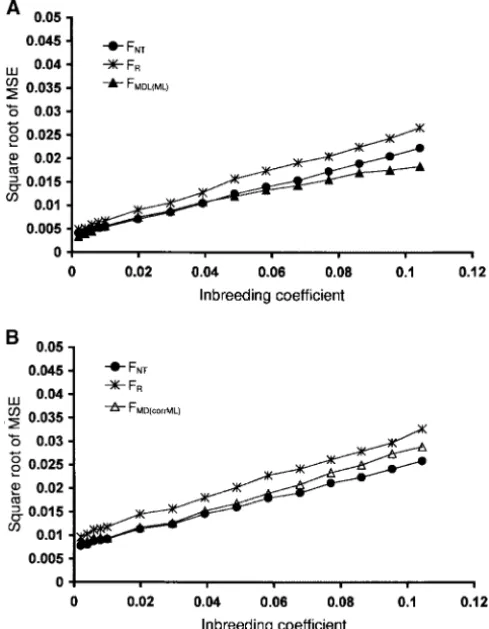
standard errors were significant (no overlapping of the Figure2.—Square root of mean square errors of inbreeding estimations: two, four, and eight founder alleles per locus are

95% confidence intervals,P⬍ 0.05).

shown. The estimations ofFtⱕ0.01 (respectivelyFtⱖ0.01) were computed over 20 loci and 1000 replications performed

Uniform founder frequencies with populations ofN⫽500,tvarying from 2 to 8 (respectively

N⫽100,tvarying from 2 to 22). Every sample size was equal

Known founder frequencies (Figures 2A, 3A, 4A, and _{to 25 individuals. In A, the true founder frequencies are known.} 5A):Square root of the mean squared error—Figure 2A:With In B, the founder sample size was set to 25 individuals. In both A and B, dotted lines show the results obtained with

uni-two founder alleles per locus (top curves),FˆNTgives the

form distributions involving four founder alleles. Solid lines

least accurate estimations (

√

MSE are the highest)

what-show the results obtained with uniform distributions involving

ever the level of drift. With four founder alleles (middle _{two (top curves) and eight (bottom curves) founder alleles.} curves) and eight founder alleles (bottom curves) per

locus, the two likelihood methodsFˆMD(ML)(Dirichlet

with-racy of every method is determined mainly by the

stan-out gene loss) andFˆMDL(ML)(Dirichlet with gene loss) diverge

from each other forⵑF⬎0.07 in the first case andF⬎ dard errors of the estimations (

√

MSE⬇SE) as long as the number of loci is not too large (⬍50).

0.04 in the second case. FˆMD(ML) shows a large loss of

accuracy with eight alleles whereasFˆMDL(ML)always gives Standard error—Figures 4A and 5A:The prediction given by Equation 14 provides a conservative basis for choos-the best estimations for anyFtvalue (with results

signifi-cantly better forF⬎0.08) and a small to medium num- ing the number and the polymorphism of markers needed to achieve a given level of precision as defined ber of alleles.

Relative bias—Figure 3A: As expected from its defini- by the variance. Indeed it is apparent that the different methods considered here are characterized by a vari-tion, FˆR shows no significant bias as is illustrated for

eight alleles (Figure 3A) and for fewer alleles (data not ance equal to or less than that predicted by the formula. In every situation encountered (four alleles, data not shown). In contrast to this result, other measures show

biases that are dependent on polymorphism and on the shown, and eight alleles, Figure 5A)FˆMDL(ML)proves to be the best with respect to the criterion of minimal vari-amount of drift.FˆNTshows significant positive bias with

two alleles (data not shown); with eight allelesFˆNT, and ance, with the difference with the theoretical reference (Equation 14) always significant forF⬎0.07. For eight alsoFˆMDL(ML), exhibit small but significant negative biases

forF⬎0.07 (confidence intervals in Figure 3A). How- alleles (Figure 5A) FˆNT performs nearly as well but is slightly less accurate [differences betweenFˆNTandFˆMDL(ML) ever, biases remain small. Therefore, except forFˆMD(ML)

Figure4.—Standard errors of inbreeding estimations: two founder alleles per locus. For the replication conditions refer

Figure3.—Relative biases of inbreeding estimations: eight to the Figure 2 legend. The straight line is the expected value founder alleles per locus. For the replication conditions refer of standard deviation from Equation 14. Confidence intervals to the Figure 2 legend. Confidence intervals are shown when of SE are shown when differences between methods are sig-the bias is significantly different from 0. In this case all methods nificant. In A the differences between methods are significant exceptFˆRshow biases significantly different from 0 for almost forFtvalues⬎0.08 [except betweenFˆRandFˆMD(ML)]. In BFˆMD(corrML)

every value ofFt. exhibits standard errors significantly lower than the standard

errors of the other methods for every value ofFtⱖ0.01.

Estimated founder frequencies (Figures 2B, 3B, 4B,

and 5B): As mentioned above, taking account of the error of estimation [

√

MSE⬇SE, except for FˆMD(corrML) computed with eight alleles per locus andFt⬎0.07].

sampling process within the founder generation needs

additional statistical treatments when the Dirichlet ap- Standard error—Figures 4B and 5B:The best method is

FˆMD(corrML) when the number of alleles is reduced (two proximation and loss of gene probabilities are

com-bined. Replacing p0,i by x0,i provides biased estimates, alleles, Figure 4B). With eight alleles per locus (Figure

5B)FˆNTis the best method with a reduction in standard with biases inversely proportional to the founder sample

size. The results given byFˆMDL(ML)are not shown. error of up to 25% for anFtvalueⵑ0.10.

The results presented in this section highlight the

Square root of the mean square error—Figure 2B:For two

alleles (top curves) a gain in accuracy was found with main drawback of the Dirichlet approximation. Biases depending on the founder polymorphism of markers the corrected likelihood estimateFˆMD(corrML). Beyond 7%

drift,FˆRis slightly better thanFˆNT. For four alleles, results and on theFtvalues appear even for a small amount of drift

(Ftⱕ0.1). This problem can be avoided when allele loss

are nearly identical for all the compared methods. With

eight allelesFˆNTturns out to be better than the others. probabilities are taken into account. These results sug-gest that this new model should be used to develop

fur-Relative bias—Figure 3B: FˆRis always unbiased (biases

were never statistically different from zero under the ther estimates, which will be more accurate when highly polymorphic markers are used. HoweverFˆMD(corrML) per-simulation conditions used in this article). BothFˆNTand

FˆMD(corrML) measures show a bias that depends on the forms well with markers exhibiting two alleles. This method should, then, be recommended when markers allelic distribution, changing in sign with the number

of alleles and the true value ofFt. In the range ofFtvalues such as single-nucleotide polymorphisms (SNPs) are used.

This method, as well as the MCMC algorithm, was considered, and discarding very low values, the relative

Figure5.—Standard errors of inbreeding estimations: eight founder alleles per locus. For the replication conditions refer

Figure6.—Square root of mean square errors: biochemical to the Figure 2 legend. The straight line is the expected value

markers. The results were performed (1000 replications,N⫽

of standard deviation from Equation 14. Confidence intervals

500 andN⫽100) with distributions of founder frequencies of SE are shown when differences between methods are

signifi-belonging to 20 biochemical markers, exhibiting an average cant. In AFˆRandFˆMD(ML)exhibit the same results. The differences

number of founder alleles of 2.5, observed within cattle breeds betweenFˆRandFˆMDL(ML)are significant forFtvalues⬎0.03. The

fromKantanenet al.(1999). differences betweenFˆNTand FˆMDL(ML) are significant for Ft ⬎

0.07. In BFˆNTexhibits standard errors significantly lower than the standard errors of the other methods forFt⬎0.05.

When the founder frequencies of biochemical mark-ers are estimated (Figure 6B), the likelihood approach

FˆMD(corrML)andNeiandTajima’s (1981) statistics provide the accuracy of the estimations ofN obtained with the

the best inbreeding estimations:FˆMD(corrML)is nearly the corrected maximum-likelihood method (estimations of

best for biochemical markers. As for the replications

N were derived from the estimations of Ft) was

deter-performed in the previous section, the effect of bias on mined with these data sets.

the global accuracy (

√

MSE⬇SE) is negligible. For mi-crosatellite markers (Figure 7B), the method giving the Biochemical and microsatellite founder frequencies

smallest standard error still provides the most accurate In this section the allele frequency distributions in- Festimations, in this caseFˆNT.

clude rare founder alleles and different numbers of The MCMC algorithm requires larger computation times alleles between markers. The

√

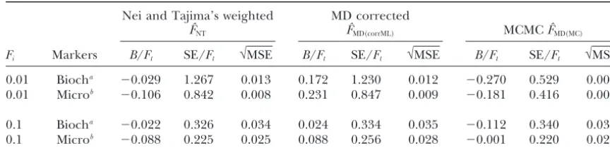
MSE in Figures 6 and 7 than the likelihood methods. The results are shown for were computed with 20 biochemical (Kantanenet al. two different values ofFt,Ft⫽0.01 andFt⫽0.1 (Table

1999) and 20 microsatellite (Lavalet al.2000) markers 1), and the number of simulations was limited toS⫽

However, even ifFˆt is unbiased,Nˆ is biased as

E(Nˆ)⬇ t 2E(Fˆt)

⫹ t

2E(Fˆt)3

Var(Fˆt). (16)

Equation 14 suggests the following estimateNˆ_⬘ofN:

Nˆ⬘ ⫽ t

2[Fˆt⫹(2/Fˆt

兺

ᐉ(n0,ᐉ⫺1))(Fˆt⫹1/m0,•⫹1/mt,•)2]

. ₍₁₇₎

The performances of these estimates are given in Tables 2 and 3. Their names are given with the same subscript as used for theFˆnotation.

The results obtained withNˆRandNˆMD(MC)are not shown since they are less accurate than those obtained with

NˆNTandNˆMD(corrML), respectively.

In every case, theNˆ⬘estimations are less biased with a smaller standard error than that of the noncorrected estimatorsNˆ. The corrected-likelihood method is more accurate than the F-statistics, for every t and for both biases and standard errors. It is more suitable to com-bine Nˆ_⬘ with the corrected maximum-likelihood ap-proach: in the last row of Table 3 (20 microsatellites),

Nˆ⬘MD(corrML) gives an unbiased estimation and leads to a decrease of 30% of the standard error ofNˆNT.

It should be mentioned here that this corrected esti-mate must be used when the experimental conditions lead to a small coefficient of variation of the estimation ofFt, since Equation 16 is accurate only when Var(Fˆt)/

Figure7.—Square root of mean square errors: microsatel- _E(Fˆ

t)2is negligible. The highest relative standard error lite markers. The results were performed (1000 replications,

ofFtin Tables 2 and 3 is⬍0.5. In practice Equation 14

N⫽500 andN⫽100) with distributions of founder

frequen-can be used to estimate the relative standard error to

cies belonging to 20 microsatellite markers, exhibiting an

aver-age number of founder alleles of four, observed within pig decide whetherNˆ⬘is relevant.

breeds fromLavalet al.(2000).

A REAL DATA SET

The numbers of simulations used to compute accuracy

We used a data set provided by J. F.Arnauld (unpub-criteria are equal to 85 (biochemical markers) and 91

lished results) to illustrate the behavior of the corrected (microsatellites) for Ft ⫽ 0.01 and equal to 100 (for

maximum-likelihood method and the MCMC algorithm both biochemical and microsatellite markers) forFt⫽

with a real data set. The population ofHelix aspersa (Gas-0.1, respectively.

tropoda: Helicidae) belongs to an intensive agricultural With biochemical and microsatellite markers,FˆMD(MC)

zone located in Brittany (northwestern France), in the was found to be significantly more accurate than FˆNT

polders of the Bay of Mont-Saint-Michel. The snail popu-andFˆMD(corrML)forFtvalues of 0.01 (the first two rows in

lation was sampled in 1998 and 2000 with 15 and 30 in-Table 1). The

√

MSE is almost halved in every case. For

dividuals, respectively. The estimations ofFtandNwere

Ft ⫽ 0.1 the MCMC algorithm does not give the same

computed with four microsatellite markers, exhibiting large gain in accuracy. There are no significant

differ-5, 6, 8, and 12 alleles in the founder generation, respec-ences among the three methods. The MCMC algorithm

tively. allows us to compute the posterior marginal distribution

The estimations ofFtobtained withFˆNT,FˆR, andFˆMD(corrML) of the parameter of interest,f(Ft|m0,mt) (Figures 8 and

are equal to 0.011, 0.016, and 0.032, respectively. Their 9;Ft⫽0.01 andFt ⫽0.1, respectively).

coefficients of variation, computed from Equation 14, Estimation of N: These data sets were also used to

are equal to 1.715, 1.264, and 1 respectively. With such obtain estimations of the effective population size since

coefficients of variation Nˆ⬘ cannot be used. We

esti-t is known (and small) and biases ofFestimations are

mated the effective size from Equation 15 assuming one small. ForFtbetween 0.01 and 0.1 (a simulated

popula-generation per year (Madec et al.2000). The estima-tion ofN⫽100) estimations ofNcan be simply obtained

tions ofNobtained withNeiandTajima’s (1981), Rey-from

noldset al.’s (1983), and the corrected maximum-likeli-hood methods are equal to 88, 62, and 31 individuals,

Nˆ ⬇ t

2Fˆt

. ₍₁₅₎

TABLE 1

Estimation ofFt⫽0.01 andFt⫽0.1 computed with the MCMC algorithm from biochemical and

microsatellite markers

Nei and Tajima’s weighted MD corrected

FˆNT FˆMD(corrML) MCMCFˆMD(MC)

Fi Markers B/Ft SE/Ft √MSE B/Ft SE/Ft √MSE B/Ft SE/Ft √MSE

0.01 Biocha _{⫺0.029 1.267 0.013 0.172 1.230 0.012 ⫺0.270 0.529 0.006}

0.01 Microb ⫺_{0.106 0.842 0.008 0.231 0.847 0.009} ⫺_{0.181 0.416 0.005}

0.1 Biocha _{⫺0.022 0.326 0.034 0.024 0.334 0.035 ⫺0.112 0.340 0.037}

0.1 Microb _{⫺0.088 0.225 0.025 0.088 0.256 0.028 ⫺0.001 0.220 0.023}

The estimations ofFtwere computed with the simulated data sets presented in Figures 6B and 7B but in every data set only the first 100 simulations were used. Vague priors␣0⫽1,a⫽2, andb⫽250 were chosen.

For every simulation the total number of iterations was set to 200,000, and only the last 100,000 were used to computeFˆMD(MC). We kept the same parameters (0.4, 4, and 25 forbu,ag, andbg, respectively, forFt⫽0.01; 0.5, 1, and 10 forbu,ag, andbg, respectively, forFt⫽0.1) for all simulations and we discarded simulations in which convergence is of doubtful validity (the percentage of accepted values⬍5). The number of simulations used to compute accuracy criteria is equal to 85 (biochemical markers) and 91 (microsatellites) forFt⫽0.01 and equal to 100 (for both biochemical and microsatellite markers) forFt⫽0.1, respectively.

a_{Biochemical markers.}

b_{Microsatellite markers.}

The MCMC estimations of Ft and of the coefficient comparison with the standard errors. To illustrate this

point whenFt⫽0.08, markers exhibit eight alleles, and

of variation (computed with the standard error obtained

from the marginal posterior distribution of Ft, Figure founder allele frequencies are exactly known, ⬎200

markers are needed for the unbiasedFˆRstatistic to out-10) are equal to 0.007 and 0.857, respectively.

performNeiandTajima’s (1981) method. Hence work-ing with measures with a low bias may be an advantage

DISCUSSION

when the level of inbreeding is low.

It must be stressed that this conclusion is quite differ-Since many different methods and situations were

ent when we consider the distance between two different investigated in this study, a summary table (Table 4) is

breeds. Indeed, the values of distances are often⬎0.1. given to highlight the main results obtained when the

Methods such asFˆNTand similar statistics as well as likeli-founder frequencies are estimated with a limited likeli-founder

hood estimates show nonnegligible biases when allele sample size (here 25 individuals), the situation most

numbers andFtvalues are large and therefore cannot

widely found in an experimental scheme.

be recommended on the basis of this work. Unbiased Scope of the present work:The scope of this article

methods such asReynoldset al.’s (1983) distance would was limited to a short-term investigation. The

compari-be preferred in such cases (Lavalet al.2002). sons of methods are based on an expected increase in

For dominant markers such as randomly amplified inbreeding of 10% or less, which corresponds to 10

gen-polymorphic DNA or amplified fragment length poly-erations for a population of 50 individuals. This seemed

morphism, allelic frequencies can be estimated with the a realistic timescale since the validity of the assumption

square root rule from the frequencies of absence of of no mutation may be questionable for longer time

bands and can be used to estimateFt, keeping in mind

intervals. The number of markers used was 20, which is

that a deviation from the Hardy-Weinberg proportions a common value found in practical (MacHugh et al.

leads to biased maximum-likelihood estimations of al-1997;Moazami-Goudarziet al.1997;Lavalet al.2000)

lelic frequencies. Some software (Arlequin,Schneider and theoretical studies (Berthier et al. 2002). This

et al.2000) provide better estimations of allelic frequen-allows the comparisons of methods made in the present

cies for dominant markers by using an expectation-max-study to be useful for experiments currently performed.

imization algorithm (ExcoffierandSlatkin1995). Increasing the number of markers to get a better

es-Performances of various estimates ofFtwere sensitive

timate of drift, which reduces the standard error around

to the total number of alleles over loci (Equation 14). the expectation but not around the true value, requires

Considering biallelic markers, SNPs seem to be full of the use of unbiased measures. Bias becomes a significant

potential (Vignalet al.2002) since their low numbers consideration when the number of alleles is large, and

of alleles can be counterbalanced by the high number analytical corrections forFˆNTcould be derived to avoid

of SNPs found in the whole genome. As a consequence this bias. In practice, however, this may be not crucial

the assumption of independence between loci does not since with the number of markers commonly used and

Figure 8.—Histogram and kernel density estimate of MCMC drawings in the posterior distribution of the

inbreed-Figure 9.—Histogram and kernel density estimate of ing coefficient, forFt⫽0.01. We kept the same parameters

MCMC drawings in the posterior distribution of the inbreed-as in Table 1. A and B were computed with one simulation

ing coefficient, forFt⫽0.1. We kept the same parameters as involving 20 biochemical markers and one simulation

involv-in Table 1. A and B were computed with one simulation involv- in-ing 20 microsatellite markers, respectively. For biochemical

volving 20 biochemical markers and one simulation involving markers the mean and the standard error are equal to 0.0062

20 microsatellite markers, respectively. For biochemical mark-and 0.0046, respectively, mark-and the percentage of accepted

val-ers the mean and the standard error are equal to 0.093 and ues of theAtparameter by the Metropolis-Hasting algorithm

0.03, respectively, and the percentage of accepted values of is equal to 19%. For microsatellite markers the mean and the

theAtparameter by the Metropolis-Hasting algorithm is equal standard error are equal to 0.0065 and 0.0046, respectively,

to 23%. For microsatellite markers the mean and the standard and the percentage of accepted values of theAtparameter is

error are equal to 0.093 and 0.023, respectively, and the per-equal to 17%.

centage of accepted values of theAtparameter is equal to 27%.

The theoretical prediction (Equation 14), although

computed under the assumption of the statistical inde- alleles per locus). More work is needed to quantify the influence of nonindependence of loci on the variances pendence of loci (linkage disequilibrium remains null),

seems to be a conservative estimate of the variance of of the estimates.

Analytical approximation: We derived an approxi-the optimizedF-statistics (Equation 13) and of the other

measures considered. With a real data set in which some mate likelihood by using the Dirichlet approximation of conditional allele frequency distribution. Comparisons be-markers are in linkage disequilibrium, the expected

standard error cannot be computed easily. Some prelim- tween likelihood methods computed when true founder frequencies are known and theF-statistics (unbiased like inary simulations have been undertaken with 100

indi-viduals, 22 generations, and 20 highly polymorphic loci FˆR and with a small variance likeFˆNT) indicate that the MD approximation model is relevant when the polymor-(20 founder alleles per locus), with a recombination

raterbetween them varying from 0.5 to 0.001. Results phism of markers is low.

When factors enhance the probability that alleles may show that the variance of theFRestimate is not affected

by linkage between loci as long asr⬎0.1. The standard be lost (high polymorphism leading to the occurrence of rare founder alleles and intermediate and high levels deviation is increased by 17% ifr⫽ 0.05 and by 155%

rele-TABLE 2

Estimation ofN⫽100 from biochemical markers

Nei and Tajima weighted MD corrected

NˆNT(15) Nˆ⬘NT(17) NˆMD(corrML)(15) Nˆ⬘MD(corrML)(17)

Ft t d ␮ ␴ d⬘ ␮ ␴ d⬘ ␮ ␴ d⬘ ␮ ␴ d⬘

0.058 12 2 137 115 1 99 40 0 130 87 2 94 39 0

0.067 14 0 132 103 0 101 41 0 129 101 0 100 40 0

0.077 16 2 126 78 2 103 42 1 123 62 1 101 40 1

0.086 18 0 124 67 0 103 42 0 121 61 0 102 39 0

0.095 20 0 123 65 0 104 42 0 120 57 0 102 38 0

0.100 22 0 119 49 0 103 36 0 116 44 0 101 33 0

The estimations of effective sizes were computed with the simulated data set presented in Figure 6B but restricted to the simulated evolution of the population of 100 individuals.␮is the mean and␴is the standard error.tis the number of generations from the founder generation. If at least one method provided values

⬎50⫻N⫽5000 (WilliamsonandSlatkin1999) as well as negative values the simulation was discarded for the correspondingt(dandd⬘are, respectively, the total and per method numbers of discarded runs). In ad-dition, when the number of discarded runs overstepped 10 (1%) the entire issue for this number of generations was removed from the table. The names of theNestimates are given by the same subscripts as used for theF

notations.

vant. Several levels of approximations were used, to cir- Combining probabilities of losses and a mixture of distri-butions in model MDL allowed the best estimates to be cumvent the combinatorial problems raised by the exact

coalescent approach when the number of alleles in- obtained when using initial known frequencies (Figure 2A). The advantage over other methods seems to be uni-creases. Likelihoods and posterior probabilities were

derived by means of a Dirichlet model and probabilities form over all considered cases, and the most pronounced improvement concerns the variance ofF estimates, al-of fixation and loss al-of alleles made use al-of a simple

ap-proximation. The latter was previously checked (Chev- though the gain seems to be less for a large number of alleles.

alet2000) and should not induce much error in the

short-term evolution considered here. The Dirichlet ap- The latter observation suggests that the combined approximation becomes less accurate for more than proximation may be more sensitive. The simpler version

(model MD) makes use of a single distribution that does eight alleles per loci. It may be suggested that the choice of the Dirichlet distributions used for transient allele not allow for null frequencies of alleles. Indeed, the

be-havior of the corresponding estimate (FˆMD(ML)) observed frequencies (appendix a) is the most sensitive step since—considering the first two moments of distribu-in Figure 2A shows the deleterious effects of distribu-increasdistribu-ing

drift or number of alleles, with both effects increasing tions—it can be proved that it is not possible to equate the true mixture (Equation 5) to the mixture of Dirich-the probabilities that some alleles may be lost by drift.

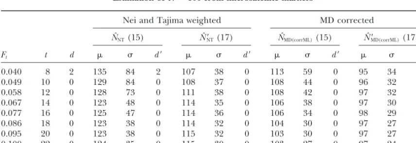
TABLE 3

Estimation ofN⫽100 from microsatellite markers

Nei and Tajima weighted MD corrected

NˆNT(15) Nˆ⬘NT(17) NˆMD(corrML)(15) Nˆ⬘MD(corrML)(17)

Ft t d ␮ ␴ d⬘ ␮ ␴ d⬘ ␮ ␴ d⬘ ␮ ␴ d⬘

0.040 8 2 135 84 2 107 38 0 113 59 0 95 34 0

0.049 10 0 129 84 0 108 37 0 108 44 0 96 32 0

0.058 12 0 128 73 0 111 38 0 108 42 0 97 32 0

0.067 14 0 123 48 0 114 35 0 106 38 0 97 30 0

0.077 16 0 125 47 0 114 36 0 106 34 0 98 29 0

0.086 18 0 123 38 0 114 32 0 104 30 0 97 27 0

0.095 20 0 123 38 0 115 32 0 103 30 0 97 27 0

0.100 22 0 124 35 0 115 30 0 103 27 0 97 24 0

Initial sampling:Precision in the estimation of founder allele frequencies is a key to accurately estimate the amount of drift. For example, the best estimate obtained with exact biochemical founder frequencies [Figure 6A,

FˆMDL(ML)estimate] shows the same mean square error as the best estimate possible with microsatellite markers sam-pled in the founder generation (Figure 7B,FˆNTestimate). As mentioned above in experimental schemes applied to domestic breeds all founder animals are known and can be sampled. In this special case, we have shown that it is possible to derive a valuable approximation of the drift process, which allows improvements of Ft

estima-tion to be obtained with both biochemical and microsa-tellites markers. The gain is significant for intermediate values of Ft (in the range of 5–10%) and if the mean

Figure 10.—Histogram and kernel density estimate of

number of alleles is not too large. From a practical point

MCMC drawings in the posterior distribution of the

inbreed-of view concerning natural populations the methods

ing coefficient, for a French snail population. The parameters

of the prior distribution are equal to those presented in based on this MDL model might be used when the

Table 1. The parameters of the candidate generating densities _{founder sample is large (up to 100 individuals). The bias} (bu⫽0.4,ag⫽8, andbg⫽20) and the number of replicates _{of the maximum-likelihood estimates, which is inversely} (500,000 with a burn-in period of 150,000 replicates) were

em-proportional to the founder sample size (data not

pirically chosen to give an optimal convergence of the chains

shown), tends to be small in front of the standard error.

of theAtandp0,i; 25% (respectively 10%) of the sampled values

of theAtparameter (respectively the founder frequenciesp0,i) For small founder sample sizes no method was found

are accepted by the Metropolis algorithm (Robert 1996). _{to be consistently better than the others over all the}

Because of the small number of markers (four markers) the _{situations tested. Introducing the allele loss probabilities} convergence of chains needs large numbers of replicates to be

in the Dirichlet model is hardly tractable in this case

completed (the number of replicates used here is significantly

and we kept this for future work. However, the methods

higher than those used with the simulated data sets; Table 1).

The mean and the standard error are equal to 0.007 and based on the Dirichlet model without allele loss greatly

0.006, respectively. _{improve the estimation of the amount of drift in several}

interesting situations.

The corrected maximum-likelihood methods (FˆMD(corrML)) let distributions that yields Equation 8. Other parameter _{and the MCMC algorithm should be preferred when} adjustments, such as using exact conditional expectations _{markers of low polymorphism are used, a situation that} (appendix a) rather than the simplified expression of _{may be of importance with the advent of the SNP} mark-Equation 7, and adjusting the dispersion parameters (A) _{ers. Using estimations of founder frequencies can lead} for each transient stateS, might give a better account of _{to biased F}

t estimations with the maximum-likelihood

drift for mid- or long-term processes. At the same time _{method based on the MD model but we have shown} this should avoid the combinatorial problem driven by _{that this problem can be solved simply with a heuristic} a large number of alleles in the exact coalescence. _{correction. This bias correction gives more accurate}

estimations than the F-statistics give without changing the standard error of the maximum-likelihood estimate.

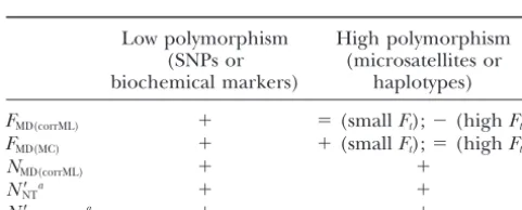
TABLE 4

In contrast, the MCMC algorithm greatly reduces the

Advantage of each method as a function of the polymorphism _{standard error of the maximum-likelihood estimate.}

Us-of markers used and _{ing this algorithm, which performs a numerical}

integra-with moderate founder sample sizes

tion of the nuisance parameters (herep0), is the most

relevant when a large part of this standard error is due

Low polymorphism High polymorphism

to the sampling in the founder generation, as was the

(SNPs or (microsatellites or

case for small Ft. We can deduce from Equation 14

biochemical markers) haplotypes)

that the sampling process is largely responsible for the FMD(corrML) ⫹ ⫽(smallFt);⫺(highFt)

decrease of the accuracy of estimations whenFtis small:

FMD(MC) ⫹ ⫹(smallFt);⫽(highFt)

the relative standard error SEt/Ft becomes large when

NMD(corrML) ⫹ ⫹

Fttends to 0 [the part depending on 1/(m0,•) is inversely

N⬘NTa ⫹ ⫹

proportional toFt].

N⬘MD(corrML)a ⫹ ⫹

The analysis of the French snail population shows ⫺, less accurate than the bestF-statistic;⫽, as accurate as

that the MCMC algorithm can be applied to a real data

the bestF-statistic;⫹, more accurate than the bestF-statistic.

set. The Markov chain well converges and the estimation

a_{The N}⬘ _{estimator can be used when the coefficient of}

by the other approaches, suggesting that the results given be used to analyze multiple data sets obtained by way of simulation. The consensus (identical for all the sim-by the MCMC algorithm are consistent. The MCMC

al-gorithm presented here is based on model MD and is ulations performed) values of the parameters of the candidate generating densities can be empirically deter-therefore affected by factors that enhance the

probabil-ity that alleles are lost: the presence of rare alleles in mined to obtain optimal convergences of the MCMC algorithm for most simulations. Although the computa-the founder sample, highly polymorphic markers, and

values of inbreeding⬇0.1. For this reason the MCMC tion time required for each simulation is reasonable (e.g., 5 min with 20 microsatellites on a Unix Sun oper-algorithm does not bring significant improvement with

this range of inbreeding values. The simulations made ating system with a processor of 480 MHz), this is still a limitation withⵑ10,000–100,000 simulations. Neverthe-with the known founder frequencies show that the

stan-dard error ofFˆMDL(ML)is always smaller than the standard less, computation times might be improved with multipro-error ofFˆMD(ML). This suggests that efforts should be made cessing computations using more powerful processors. to implement a MCMC algorithm based on the model Estimation of effective sizes:To compare the perfor-MDL, although analysis may be difficult and substantial mances of our estimates to the maximum-likelihood computation times may be required to analyze large method developed byWilliamsonandSlatkin(1999) multiple data sets. we performed 1000 simulations, keeping the same pa-Nevertheless, since for Ft ⫽0.1 the algorithm based rameters as they used in the third line of their Table 1,

on the model MD remains as accurate as the best i.e., a population of 25 individuals evolving during four

F-statistics, it can be used even with polymorphic mark- generations in which samples of 50 individuals were ers (haplotypes or microsatellites). Moreover, this algo- drawn in the founder and the fourth generation, respec-rithm gives the posterior distribution of all the parame- tively. Estimations were computed with 15 diallelic mark-ters and allows us to compute statistics, such as highest ers with founder frequencies uniformly distributed. posterior probability intervals, directly from the data The mean and the standard error of 2⫻NˆNT(which rather than from approximated calculus in which unver- is the haploid size of the population as defined in their ified assumptions were made. article) between the founder and the fourth generation Simulated tests of departure from drift:As a by-prod- are equal to 64 and 44, respectively, while they are equal uct, this work will allow the distributions of theFtesti- to 68 and 43, respectively, in Table 1 ofWilliamson

mates to be computed for one locus, considering the _{andSlatkin(1999). Since our programs return similar} pure genetic drift model as the null hypothesis. This _{results forNeiandTajima’s (1981) statistics a} compari-provides a way to test for deviations from drift, using _{son can be made. The gain in accuracy obtained with} the comparison between the value ofFtestimated from the maximum-likelihood methods ofWilliamsonand

allele frequency changes and the distribution of theFt Slatkinis interesting: mean and the standard error are

estimates obtained from computer simulations (assum- _{equal to 62 and 35, respectively. Our corrected} maxi-ing panmixia or usmaxi-ing pedigree information when it is _{mum-likelihood estimate computed from Equation 15} available). Such simulation-based tests may be helpful _[Nˆ_{MD(corrML)] seems to be as upward biased with a smaller}

to detect parts of the genome that are under the influ- _{standard error: 54 and 26 for mean and standard error,} ence of selection or of any departure from drift. _{respectively. The estimations exhibit smaller standard} As discussed inWilliamsonandSlatkin(1999) and _{errors whatever the method computed from Equation} Andersonet al.(2000), methods based on the complete _{17. The mean and standard error of the 2 *N}ˆ_{⬘NTestimate}

enumeration of all possible genetic states of a population _{are equal to 48 and 25, respectively. The 2 *N}ˆ_{MD(corrML)⬘}

(hidden Markov chain as well as coalescent approaches; _{estimate gives a mean and a standard error equal to 52} Berthieret al.2002) require intensive computation times. _{and 25, respectively. These results suggest that it would} Although these approaches are valuable, they are diffi- _{be advantageous to combine the methods recently} pro-cult to apply with multiple simulated data sets:ⵑ10,000– _{posed (WilliamsonandSlatkin1999;Berthieret al.} 100,000 simulations are needed to get the null distribu- _{2002) with theNˆ⬘estimate. A comparative study should} tion used to detect a marker under selection. _{be made to confirm this.}

Using analytical approximations allows substantial _{Other related situations:It should be noted that all} cuts in computation times. The corrected-likelihood _{the likelihood and Bayesian (MCMC algorithm)} meth-method might easily be used in such simulation-based _{ods presented in this article can be extended to include} tests with markers expected to be largely disseminated _{several sampling regimes. For example, a situation that} on the whole genome like the SNP markers. Moreover, _{occurs in practice is where animals are sampled and} with a single marker exhibiting two founder alleles (a _{genotyped at several points in time as described in} common SNP) andFtvalues⬎0.06 the standard error of _{Andersonet al.(2000). Data can be treated time interval}

FˆMD(corrML)is almost one-half that ofFˆR(data not shown), _{by time interval, or a single likelihood may be written,} which is the most accurate F-statistic in this situation _{taking the whole process into account,}

(Figure 2B).