Substructure Model for Concrete Behavior Simulation under Cyclic Multiaxial Loading

SUBSTRUCTURE MODEL FOR CONCRETE BEHAVIOR

SIMULATION UNDER CYCLIC MULTIAXIAL

LOADING

A.A. Khosroshahi and S.A. Sadrnejad*

Department of Civil Engineering, K.N. Toosi University of Technology P.O. Box 15878-4416, Tehran, Iran

[email protected] - [email protected]

*Corresponding Author

(Received: August 17, 2006 – Accepted in Revised Form: May 9, 2008)

Abstract This paper proposes a framework for the constitutive model based on the semi-micromechanical aspects of plasticity, including damage progress for simulating behavior of concrete under multiaxial loading. This model is aimed to be used in plastic and fracture analysis of both regular and reinforced concrete structures, for the framework of sample plane crack approach. This model uses multilaminated framework with sub-loading surface to provide isotropic and kinematics hardening/softening in the ascending/descending branches of loading. In multilaminated framework a relation between stress/strain and yield function on planes of various orientation is defined and stress/strain path history for each plane is kept for a sequence of future analysis. Four basic stress states including compression-shear with increase/decrease in the compression/shear ratio,tension-shear and pure compression are defined and the constitutive law for each plane is derived from the most influenced combination of stress states. With using sub-loading aspect of the surface, the kinematics and isotropic hardening are applied to the model to make it capable of simulating the behavior under any stress path, such as cyclic loading in the ascending/descending branch of loading. Based on the experimental results of the literature, the model parameters are calibrated. The model results under monotonic loading and also different states of cyclic loadings such as uniaxial compression, tension, alternate compression tension, shear and triaxial compression are compared with experimental results that shows the capability of the model.

Keywords Concrete, Multilaminate, Microplane, Elastoplastic, FEM, Substructure, Fracture

ﻩﺪﻴﻜﭼ

ﺑﻮﭼﺭﺎﻬﭼﻪﺋﺍﺭﺍﻪﺑﻪﻟﺎﻘﻣﻦﻳﺍ ﻱﺍﺮﺑﻲ

ﻡﻮﻬﻔﻣﺱﺎﺳﺍﺮﺑﻱﺭﺎﺘﺧﺎﺳﻱﻮﮕﻟﺍ ﺒﺷ

ﻬ ﺰﻳﺭﻪ

ﺖﻓﺮﺸﻴﭘﻞﻣﺎﺷﻱﺮﻴﻤﺧ

ﺭﻮـﺤﻣﺪـﻨﭼﻱﺭﺍﺬﮔﺭﺎـﺑﺖﺤﺗﻦـﺘﺑﺭﺎﺘﻓﺭﻱﺯﺎﺳﻪﻴﺒﺷﻱﺍﺮﺑﻲﮔﺪﻳﺩﺐﻴﺳﺁ

ﻲﻣﻱ

ﺩﺯﺍﺩﺮﭘ

.

ﻩﺩﺎﻔﺘﺳﺍﻑﺪﻫﻪﺑﻮﮕﻟﺍﻦﻳﺍ

ﺕﺎـﺤﻔﺻ ﻱﻭﺭ ﻙﺮﺗ ﺐﻳﺮﻘﺗ ﺏﻮﭼﺭﺎﻬﭼ ﺭﺩ ﺢﻠﺴﻣ ﻲﻨﺘﺑ ﻱﺎﻫ ﻩﺯﺎﺳ ﻭ ﻦﺘﺑ ﺖﺴﻜﺷ ﻱﺮﻴﻤﺧ ﻱﺎﻫ ﻞﻴﻠﺤﺗ ﺭﺩ

ﻲﮔﺪﺷ ﺖﺨﺳ ﻭ ﻱﺭﺍﺬﮔﺭﺎﺑ ﺮﻳﺯ ﺢﻄﺳ ﺯﺍ ﻩﺩﺎﻔﺘﺳﺍ ﺎﺑ ﻱﺍ ﻪﺤﻔﺻ ﺪﻨﭼ ﺏﻮﭼﺭﺎﻬﭼ ﺱﺎﺳﺍﺮﺑ ﻭ ﺖﺳﺍ ﻪـﻧﻮـﻤﻧ

/

ﻡﺮﻧ

ﻲﺋﻻﺎﺑﺮـﺳ ﻱﺎـﻫ ﻪﺧﺎﺷ ﺭﺩ ﻲﺘﻛﺮﺣ ﻭ ﻥﺎــﺴﻤﻫ ﻲﮔﺪﺷ

/

ﻴﺋﺎﭘﺮـﺳ

ﻲﻣ ﻱﺭﺍﺬﮔﺭﺎﺑ ﻲﻨ

ﺪﺷﺎﺑ

.

ﺪﻨﭼ ﺏﻮﭼﺭﺎﻬﭼ ﺭﺩ

ﻱﺍ ﻪﺤﻔﺻ

ﺶﻨﺗﻦﻴﺑ ﻁﺎﺒﺗﺭﺍ

/

ﻱﺎﻫﺮﻴﺴﻣ ﻭ ﻩﺪﺷ ﻒﻳﺮﻌﺗ ﻒﻠﺘﺨﻣ ﺕﺎﻬﺟ ﺎﺑ ﺕﺎﺤﻔﺻ ﻱﻭﺭ ﻥﻼﻴﺳ ﻊﺑﺎﺗ ﻭ ﺶﻧﺮﻛ

ﺶﻨﺗﻪﭽﺨﻳﺭﺎﺗ

/

ﻲﻣﻪﺘﺷﺍﺩﻪﮕﻧ ﻞﻴﻠﺤﺗﻱﺪﻌﺑ ﻞﺣﺍﺮﻣ ﻱﺍﺮﺑﻪﺤﻔﺻﺮﻫ ﻱﺍﺮﺑﺶﻧﺮﻛ ﺩﻮﺷ

.

ﺳﺎﺳﺍﺖﻟﺎﺣﺭﺎﻬﭼ ﯽ

ﺶﻨﺗ

ﺶﻳﺍﺰﻓﺍ ﺎﺑﺵﺮﺑ ﺭﺎﺸﻓﻞﻣﺎﺷ

/

ﺭﺎﺸﻓﺖﺒﺴﻧﺭﺩ ﺶﻫﺎﻛ

/

ﺑ ،ﺵﺮ ﺶﺸﻛ

-ﻥﻮﻧﺎﻗ ﻭﻩﺪﺷﻒﻳﺮﻌﺗ ﺺﻟﺎﺧﺭﺎﺸﻓﻭﺵﺮﺑ

ﻲﻣﻩﺩﺭﻭﺁ ﺖﺳﺪﺑ ﺶﻨﺗﺕﻻﺎﺣﺐﻴﻛﺮﺗ ﺮﻴﺛﺎﺗﻦﻳﺮﺘﺸﻴﺑﻱﺍﺮﺑﻪﺤﻔﺻﺮﻫ ﻱﺍﺮﺑﻱﺭﺎﺘﺧﺎﺳ

ﺩﻮﺷ

.

ﻡﻮﻬﻔﻣ ﺯﺍﻩﺩﺎﻔﺘﺳﺍ ﺎﺑ

ﺭﺎﺘﻓﺭ ﻱﺯﺎﺳﻪﻴﺒﺷﻪﺑ ﺭﺩﺎﻗﻮﮕﻟﺍ ﻭﻩﺪﻳﺩﺮﮔﻝﺎﻤﻋﺍ ﻮﮕﻟﺍ ﺭﺩﻲﺘﻛﺮﺣﻭ ﻥﺎﺴﻤﻫﻲﮔﺪﺷ ﺖﺨﺳﻱﺭﺍﺬﮔﺭﺎﺑ ﺮﻳﺯ ﺢﻄﺳ ﺑﻪﻠﻤﺟﺯﺍﺶﻨﺗﺮﻴﺴﻣﺮﻫﺖﺤﺗ

ﻲﺋﻻﺎﺑﺮﺳﻱﺎﻫ ﻪﺧﺎﺷﺭﺩﻱﺍﻪﺧﺮﭼﻱﺎﻫﺭﺎ

/

ﻲﻣﻱﺭﺍﺬﮔﺭﺎﺑﻲﻨﻴﺋﺎﭘﺮﺳ ﺪﺷﺎﺑ

.

ﺱﺎﺳﺍﺮﺑ

ﻭﺪﻳﺩﺮﮔﻲﺠﻨﺳﺍﺮﻓﻮﮕﻟﺍﻲﻫﺎﮕﺸﻳﺎﻣﺯﺁﺞﻳﺎﺘﻧ ﺞـﻳﺎﺘﻧ

ﻮﮕﻟﺍ

ﻒﻠﺘﺨﻣﺕﻻﺎـﺣﻦﻴﻨﭽﻤﻫﻭﻪﻣﺎـﮔﻚﺗﻱﺭﺍﺬﮔﺭﺎـﺑﺖﺤﺗ

ﻱﺭﻮﺤﻣ ﻚﺗﺭﺎﺸﻓ ﺪﻨﻧﺎﻣ ﻱﺍﻪﺧﺮﭼ ﺭﺎﺑ

ﺭﺎﺸﻓ ،ﺶﺸﻛ،

-ﺞـﻳﺎﺘﻧ ﺎـﺑ ﻱﺭﻮـﺤﻣ ﻪﺳ ﺭﺎـﺸﻓ ﻭﺵﺮـﺑ ،ﺏﻭﺎﻨﺘﻣ ﺶﺸﻛ

ﺖﺳﺍﻮﮕﻟﺍﺖﻴﻠﺑﺎﻗﻩﺪﻨﻫﺩﻥﺎﺸﻧﻪـﻛﺪـﻳﺩﺮـﮔﻪﺴﻳﺎـﻘﻣﻲﻫﺎﮕﺸﻳﺎـﻣﺯﺁ

.

1. INTRODUCTION

A simulation of concrete behavior and fractured

loading is very significant. Several models are used in the recent years based on the stress/strain invariants, the classical approach to constitutive modeling of concrete based on direct use of stress/strain tensor, and their invariants were used in the first decade of computer programming, and there hasn’t been any more accurate modeling of concrete since. However the models based on the concrete sub-structures, such as microplane and multilaminated could improve concrete modeling specially where the concrete is non-isotropic or there is fabric property or even a crack in the concrete. The proposed model is able to predict the behavior of concrete under any arbitrary stress/strain path and final failure mechanism.

1.1. Multilaminate Concept

The concept of multilaminate is based on the numerical approximation of integration, and the distribution of a certain physical property such as strain distributed over the surface of a media. This approach can numerically be achieved by summing up the multiplication of the property values by the specified weighted coefficients for predefined points and considering as an approximate representative value over the media. Based on this framework the behavior of a three dimensional media is averaged and approximated into the appropriate summation of slipping behavior of sampling planes passing through points. Consequently, this slip feature could be representative of the real variations of strain which are taken place through the boundaries of artificial structural units. Therefore, the accuracy of the solutions is highly related to the employed constitutive relation for the frictional slip/ opening/closing gaps of a sampling point.

1.2. History of Multilaminate Framework

The concept of multilaminate approach was first proposed by Taylor in 1938 [1]. Later a theory of plasticity based on the concept of slip theory was developed by Batdorf, et al [2] and Budiansky for metals. This theory was based on the assumption that, slip in any particular orientation in the material, will develop to a plastic shear strain which depends only on the history of the corresponding component of shear stresses/strains.

Multilaminates model for rocks was developed

by Zienkiewicz, et al [3], Also Pande, et al [4] developed elasto/viscoplastic model for clays. Bazant, et al [5] developed a model called microplane model for fracture analysis of concrete. This model was proposed to describe inelastic decline of stress at increasing strain which results to from progressive development of fracture and was based on the strain control parameters and summation of stress increments on each plane with using equivalent virtual energy to obtain macro-stress.

Sadrnejad, et al [6,7] developed a multilaminate model for granular materials and in particular sands.

2. MODEL EXPLANATION

The proposed model is originally based on the multi-laminated framework for elastoplastic behavior of intact concrete, sub-structural boundaries, considering hardening/softening rule and elastic behavior of sub-structural units. It consists of the following basis:

• Constitutive equations

• Yield function and potential surface • Hardening/Softening rule

• Flow rule and consistency condition

2.1. General Constitutive Equation

From classical theory strain can be decomposed to elastic and plastic components as follow:

P ε d e ε d ε

d = +

σ d e C e ε

d =

σ d p C P ε

d =

Ce is the elastic part of compliance matrix and CP is the plastic compliance matrix. Ce is constant for different planes and is computed from elasticity theory.

The term dεP _{can be calculated from weighted}

n planes is considered as shown in Figure 1:

p i ε d . T ] ε [L n

1

i Wi

π 8 P ε

d ∑

= =

With considering dε_ip=C_ipdσ_i

dσ ]. σ L [ . p i C . T ] ε L [ n

1

i i

W π 8 P ε

d ∑

= =

] σ L .[ p i C . T ] ε L [ p i

C =

. p i C . n

1

i Wi

π 8 P

C ∑

= =

Where L_ε and L_σ are transformation matrices for strain and stresses, respectively n is number of planes. C_ip is 3 x 3 compliance matrix for plane i in the local coordinates and Cp_i is 6 x 6

compliance matrix in the global coordinate.

Cp is composed from weighted summation of p

i

C corresponding to any of the active planes, It

should be noted that Cp_i for elastic planes

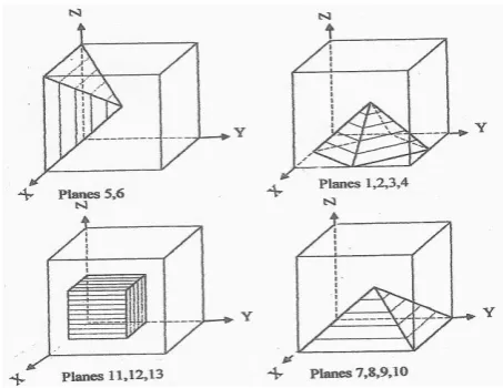
(Non-active planes) is equal Zero, Analysis shows that using 13 planes satisfy accuracy for most engineering problems. These planes are shown in the Figure 2

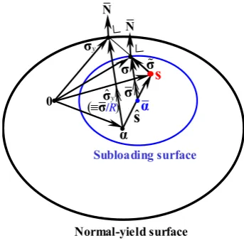
A modified Sub-loading yield surface is used in the models [8,9], for elasto-plastic behavior of planes as shown in Figure 3 sub-loading surface,which always passes through the current stress point and keeps a similar shape to the yield surface, therefore renamed as the normal-yield surface, and an orientation of similarity to the normal-yield surface. The subloading surface does not only translate but also expands/contracts with the plastic deformation.

The similarity-center S moves with a plastic deformation. Although it was fixed in the origin of stress space in the initial subloading surface model, using this concept the model has strong capability to predict isotropic and kinematics hardening behavior for loading, unloading and reloading.

2.2. Stress State on Planes

The effects of any stress/strain path over a simple typical dx,dy,dz cube element on an arbitrary sampling plane can lead to four stress/strain paths. All stress states in the material can be divided to four categories on a typical plane which are as follows:

• Compression-Shear with Increasing in the Compression

• Compression-Shear with Decreasing in the Compression

• Tension-Shear • Pure Compression

Figure 1. Multilaminate framework aspect and planes orientations.

In this framework, any form of yield criterion including crack effects may be considered for different sampling plane to any local behavior aspect, and with the summation of all planes behavior we approach the media behavior.

In most cases of element stress/strain paths the compression or tension, accompanied shear is the governing case, but for generality of the model, pure compression is considered in the model. In this way any complex form of stress/strain path is analysed into the stated four, on the planes cases and lead to proper planar behavior.

The yielding criteria proposed for the identified cases are introduced as follow:

2.2.1. Compression-shear When a plane is subjected to compression and shear in the loading path, two load pattern may exist:

™ Increasing or constant shear/compression rate with increase in the compression stress, sample of this load path is Triaxial compression test with the constant lateral pressure and increasing axial compression stress. The uniaxial compression is a special case that shear/compression ratio is constant.

™ Increasing shear/compression rate with decreasing compression stress. Sample with this load pattern is a triaxial test, when the lateral compression is decreased but axial compression is remained.

The behavior of concrete under the above load paths is not completely similar thus two separate functions are used in the equations.

2.2.1.1. Increasing Shear/Compression Rate

With Increase in the Compression Stress

In this models’ hyperbolic yield function for compressive and shear stresses is considered as follows: x σ n σ 2 z σˆ 2 y σˆ τ F(H) ) 2 n σ 3 C n (σ H C τ ) σˆ f( = + = ≤ + − = 3 C

= Material constant

F(H) = Hardening/Softening Function

m H i H , 4 v ) m H / i H ( 1 C 1 ( 2 v ) H (

F = + + ≤

m H i H , 4 v ) 1 m H / i H ( 2 C . 2 v ) m H / i H ( 1 C 1 ( 2 v ) H ( F > + − + + = 2 p zi 2 p yi 2 p xi si i

H =ε = ε +ε +ε Plastic strain

Hm = v1 = Model variable

C1,C2 Material constants

v2 Material Strength variable Hi

C Hystersis softening parameter

) i 0 H I H ( i A e ) i 0 h C 3 v . 4 C )( SIGN 1 ( 11 C ) i 0 H i H ( i A e ) i 0 H C 3 v . SIGN ( ) i 0 H i H ( i A e . 3 v Hi C − − − − − − − − =

SIGN = 1 for loading/reloading; SIGN = -1 for unloading; at the end of previous cycle CH0i = CHi

value, it may be CH0i =v3.C4 for first loading.

The term H0i is value of Hi at the end of

previous cycle in the first loading (virgin material) and it is zero. If the previous load path is pure • • • • 0 α • σ _s Subloading surface Normal-yield surface α ˆ s σ_% σ y σ ˆy σ N N )

(≡σ/R

compression H_0i =C₁₄ε_vmax.

The term Ai is cyclic parameter. At the first

loading, it is C12. Then it becomes: i 0 H . 13 C 12 C i

A = +

at the end of previous cycle.

All active planes in the state of loading such as uniaxial compression, Biaxial Compression, Triaxial Compression and also some planes in the Biaxial Compression-Tension test can be categorized in the compression-Shear state. Also it should be noted that some planes, for example plane normal to load in uniaxial compression test is in pure compression, but this plane remains elastic in the test.

2.2.1.2. Increasing Shear/Compression Rate

With Decrease in Compression Stress

In the model yield function is similar to increasing compression stress except the C3 is revised to C5 as

follows: ) H ( F ) 2 n 5 C n ( H C ) ˆ (

f σ =τ− σ + σ ≤

2.2.2.Tension-shear In this model mohr-Coloumb linear yield function between tension stress and shear stress is used:

i H 8 C e ) 4 v 2 v ( ) H ( T F x n 2 z ˆ 2 y ˆ ) H ( T F n H C ) ˆ ( f + = σ = σ σ + σ = τ ≤ σ − τ = σ

Hardening is considered in the CH as frictional

hardening/softening including degrading in the cyclic hystersis behavior also FT(Hi)represents

cohesional hardening/softening and when the crack opens the cohesional strength of material is considered as zero but the frictional strength is remained.

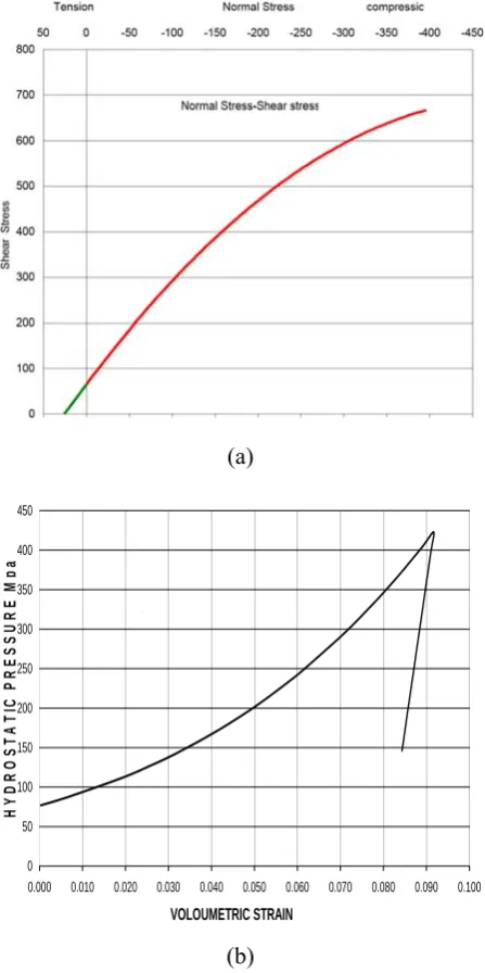
2.2.3. Pure compression state For pure compression exponential function is used as follows: 5 v c E ) v 9 C ( Exp 5 v c E

n = − ε −

σ 5 v c E ) v 9 C ( Exp c E 5 v n ) ^ (

f σ =−σ + − ε −

3 / ) z y n (

v = ε +ε +ε

ε

v Max max

v = ε

ε at end of loading

=

9

C Material constants v5 = Material variable

Figure 4 Shows this function typically

2.3. Stresses on Planes

For plane i three normal vectors is defined and stress is computed as follow:

=

σ_i stress on plane i

=

i n

r _{normal cosine of plane i} =

i

mr arbitrary vector on plane i

= il r

vector on plane i perpendicular mr_i

Vector summary are as follow

2.4. Kinematic Hardening

Kinematic

hardening is defined as below:

i i i

ˆ =σ −α σ

=

α^_i Kinematics hardening vector

7 c i H 6 C i b i i i b i ^ = σ σ = α

C6, C7, material constants

3. COMPUTATION PROCEDURE

Hi calculated from previous step. Based on the stress state of plane, the yield function is calculated. For guaranty to move in or at the surface of yield function a penalty function of U is defined as: 0 . 1 ) i H ( i F ) i ˆ ( i f i

R = σ ≤

i R ln i u i U =−

ui = V6 for shear compression state

ui = V7 for shear tension state

U is the function that relates R increment to plastic strain increment and it guarantees that Ri is to be

less than unit, It should be noted that in the numerical calculation R may be greater than one for 1-2 steps but the penalty function of U adjust it to unit even though the load step is large.

|| p i d || i U i

R& = ε

1 R 0 u 1 R 0 u 1 R 0 u 0 R for u > < = = < > = ∞ =

Similarity center S is the center of subloading in the space of stress

i S k i S 1 k i

S + = +&

⎪⎭ ⎪ ⎬ ⎫ ⎪⎩ ⎪ ⎨ ⎧ + α + σ ε

= 0FSˆ

F 1 i Ri ~ || p d || 10 C

S& &

C10 = material Constant i

S i i

~ _{=σ −}

σ

i i S

Sˆ= −α

NA N P

dε =λ Non Associate flow Rule

1 || N || ) ( f || / ) ( f N = σ ∂ σ ∂ σ ∂ σ ∂ = σ ∂ σ ∂ = ′ σ ∂ σ ∂ = ′ σ ∂ σ ∂ = ′ ) ( f ) 3 ( NA N , ) ( f ) 2 ( NA N , 15 C . ) ( f ) 1 ( NA N NA N / NA N NA

N = ′ ′

(a) 0 50 100 150 200 250 300 350 400 450

0.000 0.010 0.020 0.030 0.040 0.050 0.060 0.070 0.080 0.090 0.100

VOLOUMETRIC STRAIN H Y D R O S T A T IC PR ESSU R E M p a ` (b)

C15 = Material Constant

NA N P M

) N ( tr P

dε = σ&

⎥ ⎦ ⎤ ⎢

⎣ ⎡

⎥ ⎦ ⎤ ⎢

⎣ ⎡

σ ⎥⎦ ⎤ ⎢⎣

⎡ ′ ₊ + =

R U h F F a N tr P M

λ α = λ

=H& , a & h

Ra Sˆ U Z ) R 1 (

a = − − +

λ α

= &

Sˆ h F F 1 a R ~ C S

Z = σ+ + ′

λ

= &

i NA N p i M

) i i N ( tr p i

C = σ&

Then the Cp _{can be calculated with weighted}

summation of all planes.

∑ = π

= 13

1 i

p i C i w 8

p C

4. CALIBRATION

The parameters of models are divided into two groups, fixed parameters, that are the same for all normal concrete and need not to be calibrated for different concrete, They are parameters C1,

C2, C15 and variable parameters that should be

adjusted for each type of concrete such as V1,

V2, …, V7.

The model has been calibrated for experimental data in three stages, in the first stage the material strength under different classical load paths, such as biaxial stresses, uniaxial compression and tension, triaxial compression and shear-compression interaction is evaluated, and the parameters of most materials are defined, in the second stage the material response and strain are evaluated for many load paths such as uniaxial compression, uniaxial tension,biaxial compression,

biaxial compression-tension,triaxial compression with an increase in axial compression or decrease in lateral pressure, and also concrete behavior under pure compression. In the last stage the model is evaluated for unloading, reloading and cyclic loading.

For calibration of variable parameters(V1 to V7)

that have more effects on the model behavior, specified concrete stress-strain data for uniaxial compression, uniaxial tension and also a data for biaxial or triaxial compression strength are necessary for calibration of shear-compression and shear-tension states, and test data for pure compression should be used for calibration of model if pure compression is important. The variable parameters ranges are are shown in Table 3 (SI units).

The effect of each variable parameter on the model behavior are investigated and are as follow: V1 Shifts peak stress, increase strain

of peak stress point

V2 Increase concrete strength,

specially shear and tensile strength V3 Changes stiffness and also

compression strength

V4 Controls on the pure shear strength

and tensile strength

V5 Increase material strength in pure

compression

V6 Controls material stiffness in the

compression state

V7 Controls material stiffness in the

tension state

Fixed parameters (C1 to C15) has not changed in

different concrete and the values set can be used for normal concrete with compressive strength between 20 MPa to 60 MPa but for high strength concrete or special concrete such as fiber reinforced concrete, these values should be adjusted, It should be noted that when more accuracy is necessary some of the fixed parameter is recommended to be adjusted, for example C3 is

very important for high confinement or C13 is very

important for cyclic stress behavior. The typical values of fixed parameters for normal concrete are shown in Table 3.

behavior are investigated and are as follow:

C1,C2 Shift post peak and effect on the

residual stress

C3 Controls strength on high pressure

region specially (increasing compression)

C4 Controls stiffness degrading

C5 Controls strength on high pressure

region specially (Decreasing compression)

C6,C7 Affect on the kinematic hardening

C8 Affect on the hardening/softening

in the tension state

C9 Increase the plastic limit in pure

compression

C10 Control hystersis behavior and

residual stress

C11 Affect on the back stress in the

hystersis,

C12 and C13 Affect on the hystersis behavior

C14 Relates the pure compression

damage to other states of stress C15 Affect on the volumetric strain

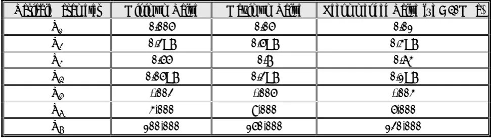
TABLE 1. Planes normal Vectors and Weights.

Weight l r mr

n

r

Plane 27/840 6 1 2 , 6 1 , 6 1 − − 0 , 2 1 , 2 1 ₋ 3 1 , 3 1 , 3 1 1 27/840 6 1 2 , 6 1 , 6 1 − − 0 , 2 1 , 2 1 3 1 , 3 1 , 3 1 ₋ 2 27/840 6 1 2 , 6 1 , 6

1 _{− +}

+ 0 , 2 1 , 2 1 3 1 , 3 1 , 3 1 − 3 27/840 6 1 2 , 6 1 , 6

1 _{− −}

− 0 , 2 1 , 2 1 ₋ 3 1 , 3 1 , 3 1 − − 4 32/840 0, 0, 1

0 , 2 1 , 2 1 ₋ 0 , 2 1 , 2 1 + 5 32/840 0, 0, 1

0 , 2 1 , 2 1 0 , 2 1 , 2 1 − 6 32/840 0, 1, 0

2 1 , 0 , 2 1 ₋ 2 1 , 0 , 2 1 + 7 32/840 0, 1, 0

2 1 , 0 , 2 1 2 1 , 0 , 2 1 − 8 32/840 1, 0, 0

2 1 , 2 1 , 0 2 1 , 2 1 , 0− 9 32/840 1, 0, 0

2 1 , 2 1 ,

0 − −

2 1 , 2 1 , 0 10 40/840 0, 0, 1

0, 1, 0 1 , 0 , 0

11

40/840 0, 0, 1

1, 0, 0 0 , 1, 0

12

40/840 1, 0, 0

0, 0, 1 0 , 0 , 1

It should be noted that if only compression-shear state is important, the strength of concrete can be adjusted with defining V2 and V3 and for adjusting

Stiffness the variable V6 should be adjusted, Thus

for compression shear state that is most important and practical case only four variable of V1, V2, V3

and V6 are necessary, For tension and tension shear

cases variable V3, V4 and V7 should be adjusted

too. V5 is only significant for pure compression

and high confinement pressure cases.

5. MODEL EVALUATION

As illustrated above the model has been evaluated

TABLE 2. Variable Parameters Ranges.

Variable Parameter Minimum Value Maximum Value Recommended Value(f”c = 40MPa)

V1 0.005 0.05 0.01

V2 0.2E7 0.5E7 0.3E7

V3 0.55 0.7 0.63

V4 0.05E7 0.2E7 0.1E7

V5 -.002 -.005 -.003

V6 3,000 8,000 5,000

V7 100,000 150,000 120,000

TABLE 3. Constant Parameters.

Constant Parameter Recommended Value (Normal Concrete)

C1 -0.01

C2 -0.001

C3 3.E-9

C4 1.8

C5 1.5E-9

C6 1.6E6

C7 0.4

C8 5000

C9 250.

C10 300

C11 200

C12 -55.

C13 -5000.

C14 0.11

0.00 0.10 0.20 0.30 0.40 0.50

0.00 0.20 0.40 0.60 0.80 1.00

Experimental-Bressler(1958) Experimental-Goode(1967) Model

Bresler[10] f 'c=28.8MPa E=38610MPa

v1=0.01

v2=0.28E7

v3=0.62

v4=0.08e7

v6=5000

v7=120000

Figure 5. Comparison of model for shear-compression experimental data Bresler [10] and Goode [11].

-1.40 -1.20 -1.00 -0.80 -0.60 -0.40 -0.20 0.00 0.20 0.40

-1.40 -1.20 -1.00 -0.80 -0.60 -0.40 -0.20 0.00 0.20 0.40

TASUJI et al Model

`

Tasuji et. al. [12] f 'c=34.5MPa ft=3.15 MPa E=31000MPa v1=0.01 v2=0.28E7 v3=0.64 v4=0.08e7 v6=5000 v7=120000

Figure 6. Comparison of model for biaxial stress experimental data, Tasuji [12].

with experimental data from literature for its calibration and evaluations in monotonic and cyclic loading

5.1. Monotonic Loading

The model is checked for different state of monotonic loadings with experimental results in the literature such as compression-shear, uniaxial compression,uniaxial

tension,Biaxial compression, biaxial compression tension and triaxial compression.

Figure 5 shows the comparison of shear compression force interaction of model prediction, experimented by Bresler, et al [10] and also Goode, et al [11] that shows the strength of the model is close to experimental result.

Tasuji, et al [12] with model prediction, The model has good fitting in compression-tension and also tension-tension region but in the compression-compression region it is little more than the experimental result.

Figure 7 shows the result of uniaxial compression test (Van Mier [13]) as predicted by model that

shows very good fitting of the whole response, also the volumetric strain results of the model is compared with experimental results that is quite fitted.

Figure 8 shows the comparison of uniaxial tension tests performed by Pettersson, et al [14],the model result is close to experimental data and has good fitting.

0.00 10.00 20.00 30.00 40.00 50.00

0.000 0.002 0.004 0.006 0.008 0.010

STRAIN

STR

E

S

S

(M

Pa)

Experimental Model

`

Van Mier [13] f 'c=38.2MPa E=38000MPa

v1=0.01

v2=0.30E7

v3=0.64

v4=0.1e7

v6=5000

v7=120000

(a)

0.00 10.00 20.00 30.00 40.00 50.00

-0.004 -0.003 -0.002 -0.001 0.000 0.001 0.002

VOLUMETRIC STRAIN

STRESS(

M

P

a)

Experimental Model

`

(b)

Figures 9 and 10 show the experimental data of Sfer [15] for triaxial test under low and high confinement with model results,They show that model predicts higher strength (7 %) in low confinement but it is close to experimental result.

5.2. Cyclic Loading

Different states of cyclic loadings such as uniaxial compression, uniaxial compression, uniaxial compression-tension and proportional and non-proportional triaxial compression are considered for evaluation of model.

0.0 1.0 2.0 3.0 4.0

0.0000 0.0001 0.0002 0.0003 0.0004 0.0005

STRAIN

ST

RE

SS

(M

Pa)

Experimental Model

Petersson [14] (a) f 'c=42.5MPa ft =3.4 MPa E=40000MPa v1=0.01 v2=0.31E7

(a)

0.0 1.0 2.0 3.0 4.0 5.0 6.0

0.0000 0.0002 0.0004 0.0006 0.0008

STRAIN

STRESS(

M

Pa

)

Experimental Model

`

Petersson[14] (b) f 'c=56.7MPa ft=4.8 MPa E=40000MPa v1=0.01 v2=0.40E7 v3=0.66 v4 0 15e7

(b)

Figure 11 shows the result of uniaxial compression cyclic loading of Sinha [16] with model prediction that shows close fitting between model result and experiment.

Figure 12 and 13 show the result of uniaxial cyclic tension and uniaxial tension alternate

compression experimental test data of Reihardt [17] with model simulation that show a good result and fitness.

Figure 14 shows the result of cyclic shear test of Eligenhause [18] with model prediction that shows good prediction.

Lateral Pressure=9MPa

0.00 20.00 40.00 60.00 80.00 100.00

0.000 0.005 0.010 0.015 0.020 0.025 0.030

STRAIN

STR

ESS(

Mpa

)

Experimental Model

Sfer et. al [15] f 'c=40MPa E=31000MPa v1=0.01 v2=0.30E7 v3=0.64

a)

(a)

0 20 40 60 80 100

-0.010 -0.005 0.000 0.005 0.010

VOLOUMETRIC STRAIN

ST

R

ESS(

MPa

)

Experimental Model

(b)

Figure 15 shows the result of hydrostatic compression of Bazant [19] with model prediction that shows very good fitting.

Figures 16 shows the comparison between Hurlbeut [20] test data for tri-axial compression with constant lateral pressure of 1Ksi (6.91 MPa)

with model prediction and in Figure 17 the result of Scavuzzo, et al [21] triaxial compression test when the axial compression decreases with an increase in the lateral pressure, as cyclic loading is shown, that illustrate good fitting of model and experimental results.

Lateral Pressure=30MPa

0.00 20.00 40.00 60.00 80.00 100.00 120.00 140.00 160.00

0.000 0.010 0.020_STRAIN0.030 0.040 0.050

STR

ESS(

M

p

a)

Experimental Model

Sfer et. al[15] f 'c=40MPa E=31000MPa v1=0.01 v2=0.30E7 v3=0.64 v4=0.1e7 v6=5000

v7=120000

(a)

0.00 25.00 50.00 75.00 100.00 125.00 150.00

-0.040 -0.030 -0.020 -0.010 0.000 0.010 0.020

VOLOUMETRIC STRAIN

ST

R

E

SS

(M

p

a

)

Experimental Model

(b)

6. CONCLUSIONS

From this research on the basis of substructure a model for simulation of concrete behavior under any stress/strain path in the multilaminate framework,

with using sub-loading surface is derived. The comparison of model with experimental data such as monotonic uniaxial compression/tension, biaxial loading, triaxial compression and hydrostatic compression, show the good simulation of model. It

0.00 5.00 10.00 15.00 20.00 25.00 30.00 35.00

0.000000 0.002000 0.004000 0.006000 0.008000

AXIAL STRAIN

AXI

AL S

TRE

SS

(M

pa

)

model-monotonic model

Experimental `

Sinha et. al. [16] f 'c=29.0MPa E=21300MPa v1=0.01 v2=0.28E7 v3=0.62

4 0 08 7

Figure 11. Comparison of model for cyclic uniaxial compression experimental data-Sinha, et al [16].

0.00 0.50 1.00 1.50 2.00 2.50 3.00

0.000 0.005 0.010 0.015 0.020 0.025 0.030 AXIAL STRAIN

A

X

IA

L

S

T

RE

SS(

M

p

a)

model-monotonic

model

Experimental `

Reinhardt et al.[18] f 'c=44.5MPa ft=2.6MPa E=34700MPa v1=0.01 v2=0.35E7 v3=0.63 v4=0.10e7 v6=5500 v7=130000

Figure 12. Comparison of model for cyclic tension experimental data-reinhardt [17].

-2.00 -1.50 -1.00 -0.50 0.00 0.50 1.00 1.50 2.00 2.50 3.00

-0.005000 0.000000 0.005000 0.010000 0.015000 0.020000 0.025000 0.030000

AXIAL STRAIN

AX

IA

L S

TRES

S(

M

pa)

model-monotonic model

Experimental

`

Reinhardt et al.[17] f 'c=44.5MPa ft=2.6MPa E=34700MPa v1=0.01 v2=0.35E7 v3=0.63 v4=0.10e7 v6=5500

Figure 13. Comparison of model for cyclic compression-Tension experimental data-reinhardt [17].

0.00 5.00 10.00 15.00

0.000 0.020 0.040 0.060

SHEAR STRAIN

SH

EA

R ST

RE

SS

(M

pa

)

model-monotonic model Experimental

`

Eligenhausen et. al. [18] f 'c=28.0MPa ft=2.75MPa E=25000MPa v1=0.01 v2=0.26E7 v3=0.61 v4=0.07e7 v6=4500 v7=120000

also shows the capability of the model to predict the behavior of concrete under any stress path such as

uniaxial compression/tension hydrostatic, loading/reloading and cyclic triaxial compression.

0.00 100.00 200.00 300.00 400.00 500.00 600.00

0.000 0.010 0.020 0.030 0.040 0.050 0.060 0.070

AXIAL STRAIN

AX

IA

L STR

ESS(

Mpa)

model

Experimental

`

Bazant et. al. [19] f 'c=45.5MPa E=35000MPa v1=0.01 v2=0.43E7 v3=0.63 v4=0.1e7 v5=0.03

6 5000

Figure 15. Comparison of model for cyclic Hydrostatic compression experimental data-Bazant, et al [19].

0.00 20.00 40.00 60.00 80.00 100.00 120.00 140.00 160.00 180.00 200.00

0.000 0.005 0.010 0.015 0.020 0.025 0.030

AXIAL STRAIN

AX

IA

L ST

RE

SS

(M

pa

) model

Experimental

`

Hurlbut et. al. [20] f 'c=19.2MPa E=17000MPa v1=0.01 v2=0.25E7 v3=0.6 v4=0.08e7

7. REFERENCES

1. Taylor, G. I. “Plastic Strain in Metals”, J. of Industrial Metals, Vol. 62,(1938), 307-324.

2. Batdorf, S. B. and Budiansky, B., “A Mathematical Theory of Plasticity Based on the Concept of Slip”,

National Advisory Committee for Aeronautics, TN 1871, (1949).

3. Zienkewics, O. C. and Pande, G. N., “Time Dependent Multi-Laminate Model of Rocks-A Numerical Study of Deformation of Rock Masses”, Int. J. of Numerical and Analytical Methods in Geomechanics, (1977),

219-247.

4. Pande, G.N. and Sharma, K. G., “Multilaminate Model of Clays-A Numerical Evaluation of the Influence of Rotation of Principal Stress Axes”, Int. J. for Numerical and Analyt. Meth. in Geomech, (1983),

397-418

5. Bazant, Z. P. and Oh, B. H., “Microplane Model for Fracture Analysis of Concrete Structures”, Proceeding Symposium on the International of Non-Nuclar Munitions with Structures, Us Air force Academy,

(1983), 49-53.

6. Sadrnejad, S. A. and Pande, G. N., “A Multilaminate Model for Sands”, Proceeding of 3rd International Symosium on Numerical Models in Geomechanics, NUMOG III, Niagara Fall, Canada, (1989), 8-11.

7. Sadrnejad, S. A., “A Sub-Loading Surface Multilaminate Model for Elastic Plastic Porous Media”,

International Journal of Engineering, Vol. 15, No.4,

(2002), 315-324.

8. Hashiguchi, K., “Elastoplastic Constitutive Equations with Extended Low Rules”, J. Fac. Agr., Kyushu University, No. 38, (1994), 279-286.

9. Hashiguchi, K., “Guide-manual for Elastoplastic Constitutive Models Comparison of Elastoplastic Constitutive Models Emphasizing on Subloading Surface Model and Bounding Surface Model”, http://www.Mech.Bpes.Kyushu-U.Ac.Jp/Index-E.Htm, Kyushu University website, (2005).

10. Bresler, B. and Pistler, K. S., “Strength of concrete under combined stresses”, J. of Am.Conc. Inst., Vol.

551, No. 9, (1958), 321-345.

11. Goode, C. D. and Helmy, M. A., “The Strength of Concrete Under Combined Shear and Direct Stress”,

Mag. of Conc. Research, Vol. 19, No. 59, (1967),

179-200.

12. Tasuji, M. E., Slate, F. O. and Nilson, A. H., “Stress-Strain Response and Fracture of Concrete in Biaxial Loading”, ACI J., (July 1978), 306-312.

13. Van Mier, J. G., “Multiaxial Strain Softening of Concrete”, J. of Mat. and Fracture, Vol. 111, No. 19, 179-200.

14. Peterson, P. E., “Crack Growth and Development of Fracture Zone in Plain Concrete and Similar Materials”, Rep. No. TVBM1006 Lund Institute of Technology, Sweden, (2001).

15. Sfer, D., Carol, I., Gettu, R. and Este, G., “Study of the Behavior of Concrete Under Triaxial Compression”,

ASCE-J. of Eng. Mech., Vol. 128, No. 2, (2002),

156-0.00 10.00 20.00 30.00 40.00 50.00 60.00 70.00 80.00

0.000000 0.002000 0.004000 0.006000 0.008000

AXIAL STRAIN

AXI

AL S

TRE

SS

(M

pa) model

Experimental

`

Scavuzzo et. al. [21] f 'c=24.2MPa E=24200MPa v1=0.01 v2=0.26E7 v3=0.61 v4=0.08e7 v6=5000

163.

16. Sinha, B. P.,Gerstel, K. H. and Tulin, L. G., “Stress-Strain Relations for Concrete Under Cyclic Loading”, J. Am. Conc. Inst, Vol. 62, No. 2, (1964), 195-210.

17. Reinhardt, H. W. and Cornelissen, H. A. W., “Post-Peak Cyclic Behaviour of Concrete in Uniaxial Tensile and Alternating Tensile and Compressive Loading”,

Cement and Concrete Research, Vol. 14, (1984),

263-270.

18. Eligenhausen, R., Popov, E. P. and Bertero, V. V, “Local Bond Stress-Slip Relationships of Deformed Bars Under Generalized Excitations”, Eartquake Engineering Research Center, College of Engineering, University of California, Bekeley, C.A. Report No.

UCB/EERC-83/23, (1983).

19. Bazant, Z. P., Xiang, Y., Adley, M., Prat, P. C. and Akers, S., “Microplane Model for Concrete II, Data Delocalization and Verification”, J. of Eng. Mech. ASCE, Vol. 3, (1996), 263-268.

20. Hurlbert, B. J., “Experimental and Computational Investigation of Strain Softening in Concrete”, Report AFOSR 80-0273, US Air Force Office of Scientific Research, University of Colorado, Boulder, U.S.A., (1985).