INSURANCE DEMAND, FINANCIAL
DEVELOPMENT AND ECONOMIC
GROWTH IN SOUTH AFRICA:
EVIDENCE FROM TODA-YAMAMOTO
CAUSALITY TEST
D. O. Olayungbo
Department of Economics, Obafemi Awolowo, University, Ile-Ife, Nigeria
Abstract
This paper examines the dynamic interactions among insurance demand, financial development and economic growth in South Africa for the period of 1970 to 2012. A Vector Error Correction Model (VECM) and Toda-Yamamoto (T-Y) causality test are used to analyze the short run and long run relationship after establishing a multivariate cointegration relation among the variables of interest. The VECM shows that, in the short run, financial development promotes insurance demand. The Toda-Yamamoto causality test supports the insurance-led and finance-led growth hypothesis with unidirectional causalities running from insurance activities and financial development to economic growth. Therefore, the results of this paper support the theory of supply leading and demand-following hypothesis for South Africa. We conclude that financial interdependence of insurance demand and financial development are crucial for growth in South Africa. The policy implication of the results is that efforts should be geared towards the implementation of policies that promotes the mutual interdependence of insurance and financial activities in South Africa.
Key words:
Insurance Demand; Financial Development; Growth; T-Y causality; South Africa.
INTRODUCTION
insurance and economic growth have also been many and mixed. For instances, studies like Soo (1996), and Ward and Zurbruegg (2000) found evidence that economic growth promotes insurance development, that is the relationship is demand-following. Others studies such as Kugler and Ofoghi (2005), Arena (2008), Haiss and Sumegi (2008), Curak, et al, (2009), Avram et al,(2010) among others found supply-leading where insurance is found to promote economic growth. However, given the contribution of both financial development and insurance to growth, empirical analysis of the relationship among insurance demand, financial development and growth is generally rare in the literature for both developed and developing countries.
Despite the apparent lack of literature on the role of insurance demand and financial development on growth, the work of Horng et al, (2012) examined the causal relationship among insurance demand, financial development and growth for Taiwan. The limitation of the work is that only the conventional ECM-type Granger (1988) short-run causality test was used in the analysis. This paper, on the other hand, adds to the literature by adopting both the short-run (ECM-type) and the long-run augmented causality test proposed by Toda and Yamamoto (1995). This is necessary as inadequate estimation technique can lead to spurious inferences and conclusions. The Toda-Yamamoto (1995) causality test provides the possibility of testing for causality between integrated variables based on asymptotic theory with or without pretest of cointegration. The results of the augmented causality are equally valid with the Wald test irrespective of the order of integration and whether there is cointegration or not. Apart from the study done for Taiwan, to the best of our knowledge no empirical paper is available in this area of economic research. Theoretically, holding of insurance policy can facilitate credit access by serving as collateral, while banks can equally provide insurance companies with liquidity facilities to enable the prompt payment of future claims to insurance policy holders.
There are reasons why this study is relevant and important in the sample country. The first is due to South Africa’s high level of insurance development in Africa. From Table 1, South Africa has the highest financial development in terms of insurance density (premium per capita) and Banking measurements in the selected African countries and African countries in general. Besides, the nature of the financial system in the country is a cross-holding where banks also act as insurers (Vivian, 1984). For instance, a bank can simultaneously mortgage bond to a client and offer the building and credit life (Vivian, 1995). Moreover, most insurance companies in South Africa hold considerable shares in the big banks (Table 2). The interrelationship between the insurance companies and the banks coupled with the financial reforms might have led to South Africa being ranked 25th in the world in 2008 ahead countries like India, Brazil
banking sector was ranked 13th out of the 53 nations (The South African Banking
Review, 1998).
In addition, the graph of insurance density and financial development in fig.1 shows that the two variables are almost moving together meaning there is likelihood of association between them. It is, therefore, against this background, that this paper examines the contribution of insurance and financial development to economic growth and their directions of causality to ascertain the one that precedes the other. The remaining part of this paper is structured as follows: section 2 provides the theoretical issues and modeling, section 3 gives the relevant literature while section 4 contains data measurement, sources and preliminary tests. Section 5 presents the empirical model, estimation results and discussions of the result while Section 6 provides conclusion and policy implications.
TABLE 1. INSURANCE DENSITY AND FINANCIAL MEASUREMENTS IN SOME SELECTED AFRICAN COUNTRIES IN 2012
Countries Life US$ non-life US$ Total Premium in US$ Premium per capita US$ Domestic Credit to private sector by financial sector % GDP US$ Bank credit to private sector % GDP US$ Broad Money as % of GDP US$ Algeria 89 1,161 1,250 32.7 68.09 38.84 61.01 Egypt 785 1,033 1,818 21.7 77.65 29.11 74.08 Kenya 436 855 1,290 30.0 52.88 36.91 51.16 Mauritius 442 213 655 498.8 113.72 100.76 100.51 Nigeria 474 1,354 1828 10.8 20.35 11.84 20.86 S. Africa* 44,787 10,084 54,871 1,124.2 188.15 71.15 75.57 Tunisia 123 694 816 76.0 80.02 72.10 67.36 Angola 57 1,083 1,140 63.1 15.74 23.27 34.51 Namibia 674 306 980 452.5 48.32 47.21 63.83 Morroco 930 1,927 2,875 76 115.36 73.25 113.90
Source: Swiss Reinsurance Company, Sigma database 2010 and World Development Indicator 2012.
Note: *South Africa export-based economy is the largest and most developed in Africa. Apart from this, the country has one of the highest per capita GDP measured in US Dollars in the African region (see Table 2, the descriptive statistics)
1970 1975 1980 1985 1990 1995 2000 2005 2010
101 102 103 104
Figure 1 The Grow th rate of Insurance density and Financial development in South Africa
Brief Overview of Insurance and Banking Structure in South Africa
The regulators in the financial sector in South Africa consist of the South African Reserve Bank (SARB), which is the South Africa’s Central Bank. The Financial Service Board (FSB) was later created to supervise non-banking financial institutions such as insurers, pension houses, brokerage firms and mutual banks. The South African banking system consists of 55 domestic banks, 5 mutual banks and 12 foreign-controlled banks while the insurance sector comprise of indigenous insurance companies which increased from 62 in 2001 to 79 insurance companies by 2010. The banking sector in South Africa was reported to be the dominant part of the financial sector with assets of 120 per cent of the GDP in 2008 (International Monetray Fund, 2008). The four biggest banks in South Africa which are ABSA, First Rand Bank, Standard Bank and Ned bank control the largest portion of 85 per cent of the total assets.
The largest contributor to life insurance is the Old Mutual, followed by other players like Salem, Liberty and Momentum. The Old Mutual is the largest life insurance company in terms of premium in Africa. In 2007, the gross written premium of the Old Mutual was US$5,359.9 million, by 2011 it has increased to US$6,447.1 million (Axco Insurance Information Services, 2012). This was followed by Momentum Group and Sanlam with premium of US$4,248.0 million and US$4,220.0 million in 2011. For the non-life, Santam Ltd is the largest with gross written premium of US$1,872.1 million in 2011. The nature of the financial system in South Africa is an extensive and intimate interrelationship of the insurance sector with the banks. There were cases of cross-holdings where banks also hold shares in insurers. As shown in Table 2, South Africa insurance companies hold a significant proportion of shares in the big South African banks.
TABLE 2. INSURANCE COMPANIES' SHARE IN SELECTED BANKS IN SOUTH AFRICA
Banks Absa Bank Ltd
Ned bank Ltd
Investec Plc
Investec Ltd
The Standard bank
Rennies Bank Ltd Insurance
companies Old-Mutual
Assurance - 52.7 4.9 7.3 20.2 9.7
Sanlam-Life
Insurance 22.7 - 2.0 3.4 5.4 6.7
Liberty-Group Ltd - - 1.6 1.8 4.9 2.6
Momentum
Life Ass. - - 1.5 1.6 1.0 -
THEORETICAL ISSUES
In the analysis of the relationship among insurance demand, financial development and economic growth, the financial system can affect economic growth in two ways. It is either through the demand-following hypothesis, which indicates that economic growth promotes the financial system or the supply-leading hypothesis that the financial system promotes economic growth (Levine, 1997; King & Levine 1993a, 1993b; Rajan & Zingales, 1998; Darrat, 1999).
Schumpeter (1911) was the first to assert the role of financial intermediaries in fund mobilization, risk management, technical innovation and growth. While insurance provides savings through premium collection that can be invested in the capital market and channeled to the productive sector, developed financial structure can equally help bring both borrowers and lenders together for growth and development. Likewise, insurance purchase reduces risk and provides liquidity for investors thereby contributing to economic growth (Watchel, 2001). Theorists such as Robinson (1952), Kuznets (1955), Stem (1989), Demetriade and Hussein (1996) are the proponents of the demand-following hypothesis. Kuznets (1955), for instance, claims that high growth rates create the incentive for consumers to demand more of financial assets and instruments due to higher returns. The increased financial demands, in turn, would generate the introduction of new financial institutions and markets to satisfy the increased demand for financial services.
Therefore, the Money in Utility (MIU) by Sidrauski (1967) and AK model by Pagano (1963) that model and describe the demand-following and the supply-leading hypotheses are presented.
Demand-Following Model
Following Sidrauski (1967), the 1Money in Utility (MIU) model that explains the
demand-following hypothesis is first presented. The model is relevant in this paper because it includes money into the utility function and helps to link monetary aggregates to growth. Thus, it helps to explain the demand-following hypothesis of economic growth and the financial services. The model assumes an infinitely lived identical agents (households and firms) and each agent takes decisions at the beginning of every period of how much to consume and how much of money to spend optimally. Individual agent maximizes their expected discounted utility-function over life-time at time 𝑡 described as :
∑ 𝛽𝑡𝑈(𝑐 𝑡, ∞
𝑡=0 𝑚𝑡) (1)
1Extensive descriptions on MIU model optimization can be found in Walsh (2010). Also, Brock (1974) and Feenstra
Where 𝛽 ∈ (0,1) is the discount factor, 𝑐𝑡= 𝐶𝑡
𝑁𝑃𝑡 as the real per capita consumption
with 𝑃𝑡 denoted by domestic price, 𝑚𝑡= 𝑀𝑡
𝑁𝑃𝑡 as real money balances and 𝑁 is the
population. The agents’ budget constraint is then given by:
𝑌𝑡+ 𝜏𝑁𝑡+ (1 − 𝛿)𝐾𝑡−1+(1+𝑖𝑡−1)𝑆𝑡−1
𝑃𝑡 +
𝑀𝑡−1
𝑃𝑡 = 𝐶𝑡+ 𝐾𝑡+
𝑀𝑡
𝑃𝑡 +
𝑆𝑡
𝑃𝑡 (2)
Eq(2) means that households earn income from previous investment which can be spent on consumption, invested as capital, saved as insurance or hold as money in the current period. Where 𝑌𝑡 = 𝐹(𝐾𝑡−1, 𝑁𝑡) is the output, 𝜏 is the population growth rate,
𝐶𝑡 is consumption, 𝐾𝑡 is the stock of capital, 𝑖𝑡−1is the past nominal interest rate, 𝑀𝑡 is the usual money balances (financial development) and 𝑆𝑡 is the insurance demand. In per capita terms, Eq. (2) can be written as:
𝑦𝑡+ 𝜏𝑡+ (1 − 𝛿)𝑘𝑡−1+(1+𝑖𝑡−1)𝑠𝑡−1+𝑚𝑡−1
1+𝜋𝑡 = 𝑐𝑡+ 𝑘𝑡+ 𝑚𝑡+ 𝑠𝑡 (3)
Eq. (3) means that the earned income of household can be spent on consumption, invested as capital, held in banks or spent on insurance purchase.
Where 𝑦𝑡= 𝑓(𝑘𝑡−1) ,and households choose 𝑐, 𝑘, 𝑠 and 𝑚 so as to maximize Eq. (1). The first order conditions for the dynamic problem using Lagrangian gives Eq. (4) to (7) as:
𝑢′(𝑐
𝑡) = 𝜆𝑡 and 𝛽𝑢′(𝑐𝑡+1) = 𝜆𝑡+1 (4)
𝜆𝑡+ 𝜆𝑡+1[𝑓′(𝑘𝑡) + (1 − 𝛿)] = 0 (5)
𝑢′(𝑚
𝑡) − 𝜆𝑡+ 𝜆𝑡+1(1+𝜋1
𝑡+1) = 0 (6)
−𝜆𝑡+ 𝜆𝑡+1(1+𝜋1+𝑖𝑡
𝑡+1) = 0 (7)
Giving up present consumption for future consumption by money yielding interest (financial development) and insurance purchase impact on growth through the capital stock expressed in Eq. (8), (9) and (10). Taking ratio of 𝑢′(𝑐𝑡) = 𝜆𝑡 and 𝛽𝑢′(𝑐𝑡+1) =
𝜆𝑡+1 in Eq. (4) gives:
𝑢′(𝑐𝑡) 𝑢′(𝑐
𝑡+1)
= 𝛽
1+𝑖𝑡1+𝜋𝑡+1 (8)
In Eq. (8), the marginal rate of substitution between present and future consumption equals the discounted value and real interest rate. Consumers are ready and willing to trade present consumption for higher future consumption due to higher returns.
From Eq. (4) and (6) we derive Eq. (9) as:
𝑢′(𝑚
𝑡) + 𝛽𝑢′(𝑐𝑡+1) (1+𝜋1
𝑡+1) = 𝑢
′(𝑐
Eq. (9) implies utility lost at present equals utility from money saved at present and additional utility from future consumption. From Eq. (4) and (5) we derive Eq. (10) as:
𝑢′(𝑐𝑡) 𝑢′(𝑐
𝑡+1) = 𝛽[𝑓 ′
(
𝑘𝑡
)
+(
1 + 𝛿)
] (10)Finally, in Eq. (10), the marginal rate of substitution between present and future consumption equals the discount value of the net marginal product of capital. Consumers are willing to trade present consumption for higher future consumption as a result of higher product of capital. This is one of the channels to which high economic growth promotes the demand of financial assets.
Supply-Leading Model
In the supply-side model, following Pagano (1993), we present an endogenous growth model alternatively called AK model. The AK model was pioneered by growth theorists such as Lucas, (1988) and Romer (1989) and the model has been used in many studies like Rebelo (1991), Jalil and Feridun (2011) and Khan (2008) among others to explain how financial assets impact on growth. The AK model is of the form:
𝑌𝑡 = 𝐴𝐾𝑡 (11)
Where Y signifies output, A is technology and K in its broad sense includes both human capital and stock of capital. This model assumes absence of diminishing returns, constant return to scale competitive economy and increasing function of capital. Capital stock evolves as follows:
𝐾𝑡 = 𝐼𝑡+ (1 − 𝛿)𝐾𝑡−1 (12)
If (1 − 𝜃) leaks from the process of savings, then savings evolve as:
𝜃𝑆𝑡−1 = 𝐼𝑡−1 (13)
From Eq. (12) and (13), the steady state growth rate equation becomes:
𝑔 = 𝐴𝜃𝑠 − 𝛿 (14)
Where 𝑔𝑡 = (𝑌𝑌𝑡
𝑡−1− 1) = (
𝐾𝑡
𝐾𝑡−1− 1) and 𝑠 =
𝑆𝑡
𝑌𝑡 . From Eq. (14), there are three channels
RELEVANT EMPIRICAL LITERATURE
As earlier stated, most of the available empirical studies are on financial development and economic growth with few insurance, financial development and growth relationships.
In Asia, Demetriades and Hussein (1996) examined the financial-led hypothesis using annual data from 1965 to 1992. The paper showed evidence of financial- led hypothesis for Sri-Lanka and that economic growth causes financial development in Pakistan. Furthermore, bi-directional causal relationships were found for India, South Korea, and Thailand. Thornton (1996) also using annual data from 1950 to 1990, found that financial-led hypothesis was evident in Nepal, Malaysia, Philippines and Thailand. Luintel and Khan (1999) also investigated the long-run causality between financial development and economic growth. Bi-directional causality was found in the six countries, namely; India, Korea, Malaysia, the Philippines, Sri Lanka and Thailand. Al-Yousif (2002) examined the relationship between financial development and growth for seven Asian countries. The Philippines and Korea supported the financial-led hypothesis, Sri Lanka and Pakistan supported the demand-following, Malaysia and Singapore had bi-directional causality while it was neutral for Thailand. Levine (1997) found that bank-based and markets-based financial markets are complimentary in providing financial services to the economy because both have positive associations with economic growth. Fase and Abma (2003) used pooled data for nine countries such as Bangladesh, India, Malaysia, Pakistan, the Philippines, Singapore, South Korea, Sri Lanka and Thailand. The paper concluded that financial development matters for growth and that causality was from financial development to growth.
In Africa, Odhiambo (2009) examined the relationship among the variables such as interest rate reforms, financial development and growth in South Africa. The results show that causal relationship exists from financial development to economic growth which is a demand-following relationship. Djoumessi (2009) examined the relationship between financial development and economic growth in Cameroon and South Africa from 970 to 2006. Both VECM and ARDL were employed. The result showed both positive contributions from financial development to economic growth in the two countries. Sunde (2012) also examined the relationship between financial sector development and economic growth in South Africa using ECM and Granger causality test for the period of 1977 to 2009. The ECM result showed that growth is explained by financial sector variables, while the granger causality shows a bi-directional causality between financial development and economic growth in South Africa.
Aziakpono (2003) examined the relationship between financial intermediation and economic growth for Botswana, Lesotho, Namibia, South Africa and Swaziland between 1980 to 2000 by using two financial indicators. In the analysis, while mixed evidence of financial intermediation are found for Botswana, strong evidence of relevance of domestic financial intermediation are found for South Africa, weak for Lesotho and Swaziland. Previous insurance-growth studies in South Africa are few. Alhassan and Fiador (2014) examined long run causal relationship between insurance penetration and economic growth for Ghana during the period of 1990 to 2010. The authors used autoregressive distributed lag (ARDL) bounds approach to cointegration by Pesaran et al, (1996, 2001). The study found a long run positive relationship between insurance penetration and growth. A unidirectional causality was found from aggregate insurance penetration to growth on one hand and life and non-life insurance penetration to growth on the other hand
Horng et al, (2012) carried out the relationship among Insurance, financial development and economic growth for Taiwan. The paper found economic growth to granger cause insurance demand and financial development to granger cause economic growth both in the short run. In summary, from the empirical literature, it is obvious that previous studies on insurance demand, financial development and economic growth in South Africa are rare.
DATA SOURCES AND VARIABLE DEFINITIONS
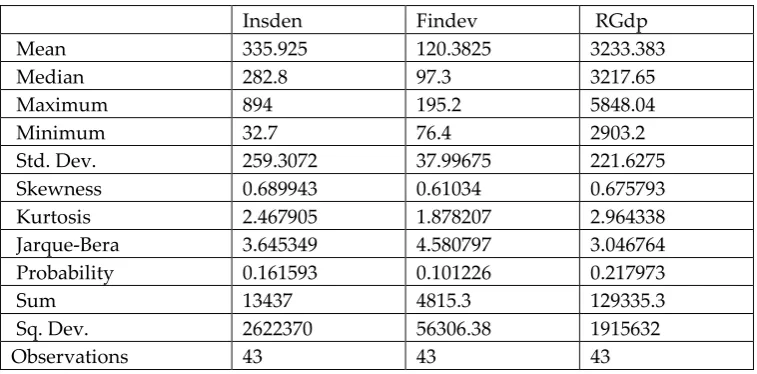
Following previous studies, such as (Ward & Zurbruegg, 2002; Esho et al, 2004; Horng et al, 2012) real GDP per capita (Rgdp) was used to measure economic growth. Financial development (Findev) was measured as ratio of M2 (broad money supply) to GDP. GDP and M2 were both measured in US dollars. Both the series for Real GDP per capita (constant 2005) and financial development were obtained from World Development Indicator (WDI, 2011). Insurance density (Insden), that is, premium per capita after adjusted for inflation, was used as a proxy for insurance demand (Brown et al, 2000) and was sourced from Swiss Reinsurance Company, Sigma Publication (2011). The data on insurance density, financial development and the GDP per capita are all measured in US dollars after adjusted for inflation. The descriptive statistics of all our series are presented in Table 3 with 43 observations. The values of the mean and median are bit close, which suggest low variability and normal distribution of the data. The closeness of the value of the kurtosis, the skewness and Jarque-Bera to zero also suggest symmetrical nature of the distribution.
TABLE 3. DESCRIPTIVE STATISTICS OF VARIABLES
Insden Findev RGdp
Mean 335.925 120.3825 3233.383
Median 282.8 97.3 3217.65
Maximum 894 195.2 5848.04
Minimum 32.7 76.4 2903.2
Std. Dev. 259.3072 37.99675 221.6275 Skewness 0.689943 0.61034 0.675793 Kurtosis 2.467905 1.878207 2.964338 Jarque-Bera 3.645349 4.580797 3.046764 Probability 0.161593 0.101226 0.217973
Sum 13437 4815.3 129335.3
Sq. Dev. 2622370 56306.38 1915632
Observations 43 43 43
Unit root Test
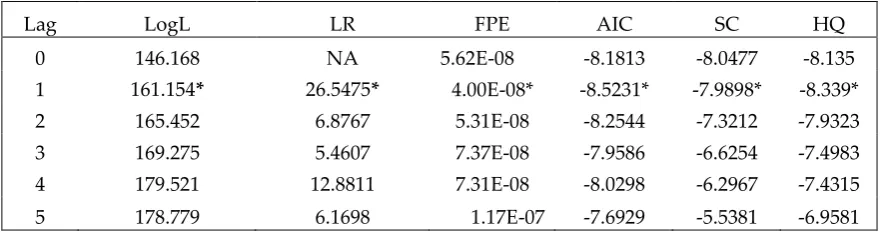
are I(1). As a consequence, the cointegration test is conducted after 1 lag length selection shown in Table 4 using the Akaike Information Criteria (AIC), Schwartz Bayesian Information Criterion (BIC), and Hannan-Quinn Criterion (HQC).
TABLE 4. UNIT ROOT RESULTS
Intercept Trend and Intercept
Variables Levels First diff Variables Level First diff. Lfindev -0.0543 -7.7150 Lfindev -2.4633 -7.8522 Linsden -1.9245 -4.6810 Linsden -0.6321 -5.2155 Lrgdp -1.6979 -3.6971 Lrgdp -1.5763 -3.7278
ADF critical values for the intercept at levels and first difference are -3.6105(1%), -2.9390 (5%),-2.6079 (10%) and while that of the trend and intercept at level and first difference are -4.2119(1%), -3.5298(5%) -3.1964(10%). All the variables are in log form.
TABLE 5. LAG LENGTH SELECTION CRITERIA
Lag LogL LR FPE AIC SC HQ
0 146.168 NA 5.62E-08 -8.1813 -8.0477 -8.135 1 161.154* 26.5475* 4.00E-08* -8.5231* -7.9898* -8.339* 2 165.452 6.8767 5.31E-08 -8.2544 -7.3212 -7.9323 3 169.275 5.4607 7.37E-08 -7.9586 -6.6254 -7.4983 4 179.521 12.8811 7.31E-08 -8.0298 -6.2967 -7.4315 5 178.779 6.1698 1.17E-07 -7.6929 -5.5381 -6.9581 LR means Likelihood Ratio, FPE is Final Prediction Error Criterion, AIC is Akaike Information Criterion, SC is Schwach Criterion, HQ is Hannan-Quinn Criterion. * signifies optimal lag length.
Cointegration test
In order to ascertain the long-run relationship among the variables, the Johansen (1991), a multivariate cointegration test is employed following previous studies such as (Demetriades & Hussein, 1996; Luintel & Khan, 1999) in VAR form as:
∆𝑦𝑡 = 𝛼 + Π𝑦𝑡−1+ ∑𝜌−1𝑖=1 Γ𝑖Δ𝑦𝑡−𝑖+ 𝜀𝑡 (15)
With the cointegration result, we expect there should be at least 3 direction of causality among the variables (Engle & Granger, 1987).
TABLE 6. JOHANSEN COINTEGRATION MLE ESTIMATES
Null Trace Stat.
Crit. 90%
Crit. 95%
Crit.
99% Null Eigen Stat.
Crit. 90%
Crit. 95%
Crit. 99%
r<=0 50.65 27.07 29.8 35.46 r<=0 24.49 18.89 21.13 25.87 r<=1 26.16 13.43 15.49 19.94 r<=1 16.22 12.3 14.26 18.52
r<=2 9.93 2.71 3.84 6.64 r<=2 9.93 2.71 3.84 6.64
Notes: 𝑟 = 𝑚 i.e no of cointegrating vectors is equal number of equation, whereas according to econometric theory (Johansen, 1991) 𝑟 < 𝑚 for the appropriate cointegrating vector should be identified.
Robustness Checks on Cointegration
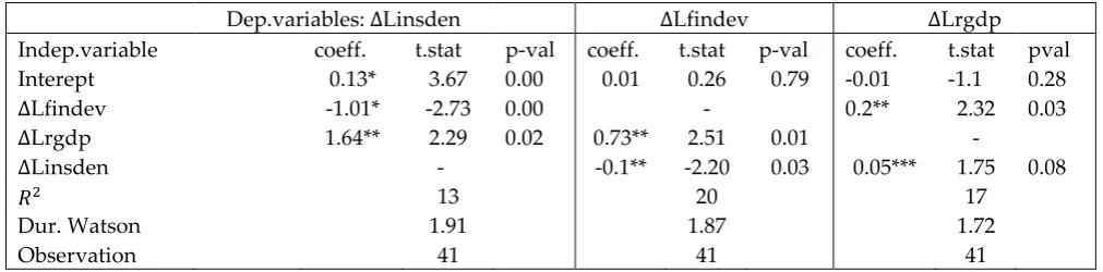
Given the small sample size of our analysis, the Johansen cointegration procedure is sensitive to wrongly reject the null hypothesis of no cointegration in small sample (Reinsel & Ahn, 1992). In order to ascertain the cointegration of the variables, the cointegration test proposed by Phillips and Hansen (1990) called the fully modified Ordinary Least Square (FMOLS) which corrects for finite-sample biases is employed. The FMOLS usually corrects for endogeneity, serial correlation and not sensitive to lag length in the regression equations (Phillips & Hansen, 1990). The FMOLS result presented in Table 7 confirms the presence of cointegration among the variables with their significant p-values and the Durbin Watson showing absence of autocorrelation. The residuals of each co integrating equations are also stationarity and not correlated.
TABLE 7. FULLY MODIFIED OLS COINTEGRATION ESTIMATE
Dep.variables: ∆Linsden ∆Lfindev ∆Lrgdp Indep.variable coeff. t.stat p-val coeff. t.stat p-val coeff. t.stat pval Interept 0.13* 3.67 0.00 0.01 0.26 0.79 -0.01 -1.1 0.28
∆Lfindev -1.01* -2.73 0.00 - 0.2** 2.32 0.03
∆Lrgdp 1.64** 2.29 0.02 0.73** 2.51 0.01 -
∆Linsden - -0.1** -2.20 0.03 0.05*** 1.75 0.08
𝑅2 13 20 17
Dur. Watson 1.91 1.87 1.72
Observation 41 41 41
*,** , and ***represent 1%, 5% and 10% significant levels.
EMPIRICAL ANALYSIS
so as to avoid invalid assumptions and model mis-selection that could result in inefficient or inconsistent inferences and policy implications.
Weak Exogeneity test
In carrying out the weak exogeneity test, a restriction is usually placed in the VECM such that in the Granger representation, the i-th row of the 𝛼 matrix is set to zero (Johansen, 1995; Harris, 1995; Urbain, 1992). Granger’s representation shows that Π =
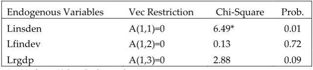
𝛼𝛽′ and that Π has reduced rank i.e 𝑟 < 𝑘 where there exists 𝑘 × 𝑟 of 𝛼 and 𝛽 each with rank 𝑟. Where 𝑟 is the number of cointegrating relations and each column of 𝛽 is a cointegrating vector. Johansen (1995) gives more exposition on the weak exogeneity test. Then, if this condition of setting the 𝛼 matrix is set to zero holds with respect to the 𝛽 parameters, the i-th endogenous variable is assumed to be weakly exogenous. Namely, A test of the null hypothesis 𝐻0: 𝛼11 = 0 is a test of weak exogeneity since a rejection of the null means log of insurance (linsden) is exogenous to the system. The same procedure is applied in our estimation. The results, shown in Table 8, indicate that the first co integrating vector is the identified vector where the insurance demand (Linsden) is the dependent variable.
TABLE 8. THE RESULTS OF THE WEAK EXOGENEITY TEST
Endogenous Variables Vec Restriction Chi-Square Prob.
Linsden A(1,1)=0 6.49* 0.01
Lfindev A(1,2)=0 0.13 0.72
Lrgdp A(1,3)=0 2.88 0.09
* signifies 5% level of significance
Vector Error Correction Model
According to Loayza and Ranciere (2006), short-term dynamic is also important as it explains the deviations of the variables from their long-run path. As a result, after identifying the appropriate co integrating vector with the weak exogeneity test, the short-run causality and dynamics are done using the identified model of the weak exogeneity test in the VECM representation as follows:
∆𝐿𝑖𝑛𝑠𝑑𝑒𝑛𝑡 = 𝜇 + 𝜑11∆𝐿𝑖𝑛𝑠𝑑𝑒𝑛𝑡−1+ 𝜑12∆𝐿𝑓𝑖𝑛𝑑𝑒𝑣𝑡−1+ 𝜑13∆𝐿𝑟𝑔𝑑𝑝𝑡−1+ 𝛼11𝐸𝐶𝑇𝑡−1+ 𝜀1𝑡 (16)
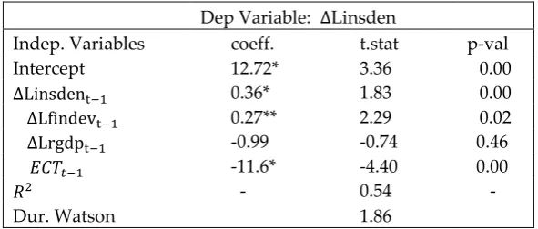
TABLE 9. ERROR-CORRECTION MODEL FOR INSURANCE DEMAND, FINANCIAL DEVELOPMENT AND GROWTH
Dep Variable: ∆Linsden Indep. Variables coeff. t.stat p-val Intercept 12.72* 3.36 0.00
∆Linsdent−1 0.36* 1.83 0.00
∆Lfindevt−1 0.27** 2.29 0.02
∆Lrgdpt−1 -0.99 -0.74 0.46
𝐸𝐶𝑇𝑡−1 -11.6* -4.40 0.00
𝑅2 - 0.54 -
Dur. Watson 1.86
*, ** and ***represent 1%, 5% and 10% significant levels. The long run normalized co integrating equation is 𝐸𝐶𝑇𝑡−1= 𝐿𝑖𝑛𝑠𝑑𝑒𝑛𝑡−1+ 0.74 𝑙𝑓𝑖𝑛𝑑𝑒𝑣𝑡−1+ 0.01𝐿𝑟𝑔𝑑𝑝𝑡−1
Toda Yamamoto Causality Test
Having established the other of integration of our data in Table 3 with the optimal lag length of 1 in Table 4, we proceed to the Toda-Yamamoto (1995) causality procedure given the model stability and non-serial correlation in the residual (Appendix). The Toda-Yamamoto (1995) procedure is a non-granger causality test with a linear restriction, null hypothesis and Wald test statistics that are asymptotically distributed as 𝜒2. The causality test does not require any prior knowledge of the order of cointegration of the variable of interest. The method proposes a causality test in the level VAR equation, by applying an augmented VAR(p + d)2 to the data. We test for the Toda-Yamamoto Granger Causality test based on the following equations:
𝑖𝑛𝑠𝑑𝑒𝑛 = 𝜙0+ ∑𝑝+𝑑𝑖=1 𝜙1𝑓𝑖𝑛𝑑𝑒𝑣 + ∑𝑝+𝑑𝑖=1 𝜙2𝑟𝑔𝑑𝑝 + 𝜀1𝑡
𝑓𝑖𝑛𝑑𝑒𝑣 = 𝛽0+ ∑𝑝+𝑑𝑖=1 𝛽1𝑖𝑛𝑠𝑑𝑒𝑛 + ∑𝑝+𝑑𝑖=1 𝛽2𝑟𝑔𝑑𝑝 + 𝜀2𝑡
𝑟𝑔𝑑𝑝 = 𝜔0+ ∑𝑝+𝑑𝑖=1 𝜔1𝑓𝑖𝑛𝑑𝑒𝑣 + ∑𝑝+𝑑𝑖=1 𝜔2𝑖𝑛𝑠𝑑𝑒𝑛 + 𝜀3𝑡 (18)
Where d is the order of integration of the variables in the VAR and p is the is number of lags. The null hypothesis that 𝐻0: 𝜙1 = 𝜙2 = 0 is a test that findev and rgdp do not granger-cause insden. Similarly, the null hypothesis that 𝐻0: 𝛽1 = 𝛽2 = 0 means insden and rgdp do not granger-cause findev and lastly, the null hypothesis that
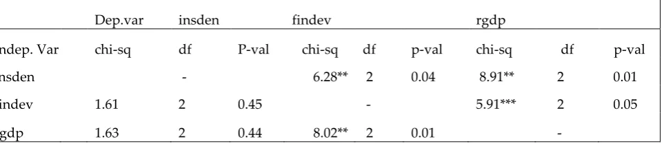
𝐻0: 𝜔1 = 𝜔2 = 0 implies findev and insden do not granger-cause rgdp. The T-Y granger causality results are presented in Table 10.
2 The lag length of 1 is found to be optimal, and the maximum number of order of integration of integration in is
TABLE 10. T-Y GRANGER CAUSALITY TEST OF INSURANCE DEMAND, FINANCIAL DEVELOPMENT AND GROWTH
Dep.var insden findev rgdp
Indep. Var chi-sq df P-val chi-sq df p-val chi-sq df p-val
insden - 6.28** 2 0.04 8.91** 2 0.01
findev 1.61 2 0.45 - 5.91*** 2 0.05
rgdp 1.63 2 0.44 8.02** 2 0.01 - *, ** and *** indicates significance level at 1%, 5% and 10%.
DISCUSSION OF RESULTS
Table 9 reports the result of the VECM with insurance demand as the dependent variable. The lagged error-correction term is significant at 1% level and correctly signed with negative value of -11.6. This implies that in the long run, the adjustment of insurance demand to changes in both economic growth and financial development is high with 116%. 1% change in both financial development and economic growth leads to 116% change in insurance demand. This result is not surprising given the high financial development and GDP per capita of South Africa relative to other African countries (see Table 1). Moreover, the short run dynamic shows that coefficients of past value of insurance demand and financial development are significant at 1% and 5% respectively. The results indicate that insurance demand responds significantly to positive changes in both its past value and financial development in the short-run. This result confirms the outstanding features in South Africa’s financial system where insurers have substantial shareholdings in the banking system and a situation of banks establishing their own insurers (Vivian, 1995). On the contrary, there is insignificant response of insurance demand to negative change in economic growth in the short run. This implies that negative short-run changes do not have significant effects on insurance demand in the sample country.
during the sample period is in line with studies like Aziakpono, (2003) and Djoumessi (2009) for South Africa. Therefore, in summary, the following findings emerge from this paper. Firstly, short-run unidirectional causalities are found to run from financial development to insurance. Secondly, long run unidirectional causality is found to run from insurance demand to financial development. Also, long-run causalities run from insurance demand and growth to financial development. Finally, a long-run causality runs from both financial development and insurance demand to economic growth.
CONCLUSION AND POLICY IMPLICATIONS
Using a three-variable model, the demand following and supply leading hypotheses are empirically tested regarding the dynamic relationship among insurance demand, financial development and economic growth in South Africa. This paper is relevant for the sample country given her high level of insurance development and the financial linkages between insurance and the financial sectors in the country. The empirical results show that there is a long run, or equilibrium relationship among insurance demand, financial development and economic growth. The VECM results show that in the short-run, financial development promotes insurance demand, while in the long-run, the causality tests reveal unidirectional causalities running from both insurance demand and economic growth to financial development. Lastly, insurance demand and financial development are equally found to granger-cause economic growth in the long-run. The result supports the insurance-led and finance-led growth hypothesis that is the supply-leading and the demand-following hypothesis in the long-run for South Africa.
REFERENCES
Alhassan, A. L. & Fiador, V. (2014). Insurance-growth nexus in Ghana: An autoregressive Distributed lag Bounds Co-integration Approach, Review of Development Finance, (http://dx.doi.org/10.1016/j.rdf.2014.05.003).
Al-Yousif, Y. K. (2002). Financial development and economic growth: another look at the evidence from developing countries, Review of Financial Economics, 11, 131-150.
Al-Zubi, K, Al-Rjoub, S. & Abu-Mhareb, E. (2006). Financial development and economic growth: New empirical evidence from the MENA countries, 1989-2001, Applied Econometrics and International Development, 6, 3-11.
Arena, M. (2008). Does Insurance Market Promote Economic Growth? A Cross-Country Study for Industrialized and Developing Countries, Journal of Risk and Insurance, 75(4), 921- 946.
Axco Insurance Information Services. (2012). (www.axcoinfo.com).
Avram, K., Nguyen, Y. & Skully, M. (2010). Insurance and Economic Growth: A Cross-Country Examination, Monash University, Department of Accounting and Finance, Working Paper.
Aziakpono, M. J. (2003). Financial Development and Economic Growth in Southern Africa, Department of Economics National University of Lesotho, P.O. Roma 180, Lesotho (http://kris-nimark.net/pdf/VARpSlides.pdf).
Brock, W. A. (1974). Money and Growth: The Case of Long-Run Perfect Foresight, International Economic Review, 15(3), 750-777.
Browne, M. J., Chung, J. & Frees, E. W. (2000). International Property-Liability Insurance Consumption, Journal of Risk and Insurance, 67, 73-90.
Budlender, D. (1984). Workmens' Compensation, South African Labor Bulletin, 9, 22-40.
Curak, M. Loncar, S. & Poposki (2009). Insurance Sector Development and Economic Growth in Transition Countries, International Research Journal of Finance and Economics, 34(1), 29-41.
Darrat, A. F. (1999). Are financial deepening and economic growth casually related? Another look at the evidence, International Economic Journal, 13, 19-35.
Dickey, D. A. & Fuller, W. A. (1979). Distribution of the Estimators for Autoregressive Time Series with a Unit Root, Journal of the American Statistical Association, 74, 427-431.
Djoumessi, E. C. (2009). Financial Development and Economic Growth: A comparative study between Cameroon and South Africa: A master Degree in Master of Commerce in economics at the University of South Africa.
Doan, T., Littermann & Sims, C. A. (1984). Forecasting and Conditional Projections Using Realistic Prior Distributions, Econometrics Reviews, 3(4), 1-100.
Engle, R. F. & Granger, C. W. J. (1987). Cointegration and error correction: representation, estimation and testing, Econometrica, 55, 251-276.
Feenstra, R. C. (1986). Functional Equivalence between Liquidity Costs and the Utility of Money, Journal of Monetary Economics, 17(2), 271-291.
Goldsmith, R. W. (1969). Financial structure and development. New Haven, CT7 Yale Univ. Press.
Haiss, P. & Sumegi, K. (2008). The relationship between insurance and Economic Growth in Europe: A Theoretical and Empirical Analysis, Empirica, 35(4), 405-431.
Harris, R. (1995). Using Cointegration Analysis in Econometric Modelling, Prentice Hall, England.
Horng, M., Chang, Y. & Wu, T. (2012). Does Insurance Demand or Financial Development promote Economic Growth? Evidence from Taiwan, Applied Economics Letters, 19(2), 105-111.
Johansen, S. (1995). Estimation and Hypothesis Testing of Cointegration Vectors in Gaussian Vector Autoregressive Models, Econometrica, 59, 1551-1580.
Khan, M. A. (2008). Financial development and economic growth in Pakistan: evidence based on Autoregressive Distributed Lag (ARDL) approach, South Asia Economic Journal, 9(2), 375-391.
King, R. G. & Levine, R. (1993a). Finance, entrepreneurship, and growth: theory and evidence, Journal Monetary Economics, 32(3), 513-542.
King, R .G. & Levine, R. (1993b). Financial and growth: Schumpeter might be right. The Quarterly Journal of Monetary Economics, 32, 513-542.
Kugler, M. & Ofoghi, R. (2005). Does Insurance Promote Economic Growth in Europe: Atheoretical and Empirical Analysis, Empirica, 35(4), 405-431.
Levine, R. (1997). Financial Development and Economic Growth: views and agenda, Journal of Economic Literature, 35, 688-726.
Levine, R., Loyaza, N. & Beck, T. (2000). Financial Intermediation and Growth: Causality and Causes, Journal of Monetary Economics, 46, 31-71.
Lewis, R. E. (1955). The Theory of Economic Growth, London, George Allen and Unwin.
Loayza, N. V & Ranciere, R. (2006). Financial Development, Financial Fragility and Growth, Journal of Money Credit and Banking, 38(4), 1051-1076.
Lutkephol, H. (1993). Introduction to Multiple Time Series Analysis, 2nd Ed.,
Springer-Verlag, N. Y.
Luintel, K. B. & Khan, M. (1999). A quantitative reassessment of the finance-growth nexus: evidence from a multivariate VAR, Journal of Development Economics, 60, 381-405.
MacKinnon, R. I. (1973). Money and capital in economic development, Washington, DC7, Brookings Institution.
Odhiambo, N. M. (2009). Interest rate liberalization, financial deepening and economic growth in South Africa:” An empirical investigation. In: Paper Presented at the Ninth Annual IBER & TLC Conference Proceedings, Las Vegas, NV, USA.
Ozturk, I. (2008). Financial development and economic growth: Empirical evidence from Turkey, Applied Econometrics and International Development, 8(1), 85-98.
Pagano, M. (1993). Financial Markets and Growth: An Overview, European Economic Review, 37(1), 613-622.
Patrick, H. T. (1966). Financial development and economic growth in undeveloped countries, Economic Development and Cultural Change, 14, 174-189.
Pei-Fen, C., Chin-Chiang, L., Chun-Ping, C. & Lee, C. (2011). How does the development of the Life Insurance Market affect Economic Growth? Some International Evidence, Journal of International Development, 24(7), 865-893.
Phillips, P. C. B. & Hansen, B. E. (1990). Statistical Inference in Instrumental Variables Regression with I(1) process, The Review of Economic Studies, 57(1), 99-125.
Rajan, R. G. & Zingales, L. (1998). Financial dependence and growth, American economic Review, 88, 559-586.
Reinsel, G. C & Ahn, S. K. (1992). Vector Autoregressive Models with Unit Roots and Reduced Rank Structure: Estimation, Likelihood Ratio Test, and Forecasting, Journal of Time Series Analysis, 13(4), 353-375.
Robinson, J. (1952). The rate of interest and other essays. London, Macmillan.
Schumpeter, J. A. (1911). The theory of economic development, Cambridge, MA7 Harvard Univ. Press.
Shaw, E. S. (1973). Financial deepening in economic development, New York7 Oxford Univ. Press.
Sidrauski, M. (1967). Rational Choice and Pattern of Growth in a Monetary economy, American Economic Review Papers and Proceedings, 30, 534-544.
Soo, H. H. (1996). Life Insurance and Economic Growth: Theoretical and Empirical Investigation. University of Nebraska, Lincohn.
South African Reserve Bank. (http://www.reservebank.co.za/). Investigation. Ph.D Dissertation, University of Nebraska, Department of Economics, Lincoln.
Stem, N. (1989). The economics of development: a survey, The Economic Journal, 597-685.
Sunde, T. (2012). Financial Sector Development and Economic Growth Nexus in South Africa, International Journal of Monetary Economics and Finance, 64-75.
Toda, H. Y. & Phillips, P. C. B. (1993). Vector Autoregressions and Causality, Econometrica, 61(6), 1367-1393.
Toda, H. Y. & Yamamoto, T. (1995). Statistical Inference in Vector Autoregressions with Possibly Integrated Processes, Journal of Econometrics, 66(1-2), 225-250.
Urbain, J. P. (1992). On Weak Exogeneity in Error Correction Models, Oxford Bulletin of Economics and Statistics, 54(2), 187-207.
Vivian, R. W. (1984). Identifying the Source of the MVA Rate Crisis, address at the Noschon Conference, Sun City, Republic of South Africa (May 8).
Ward, D. & Zurbruegg, R. (2000). Does Insurance Promote Economic Growth? Evidence from OECD Countries? The Journal of Risk and Insurance, 67(4), 489-506.
Wachtel, P. (2001). Growth and Finance: What do we know and How do we know it?, International Finance, 4(3), 335-362.
APPENDIX
FIGURE 1. INVERSE ROOTS OF AR CHARACTERISTIC POLYNOMIAL
Note: The dots shows that no variable lies outside the unit circle and this confirms the stability of the estimated VAR model.
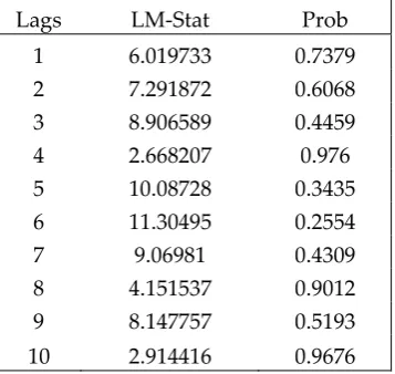
TABLE 1. RESIDUAL SERIAL CORRELATION LAGRANGE MULTIPLIER (LM)TEST
Lags LM-Stat Prob 1 6.019733 0.7379 2 7.291872 0.6068 3 8.906589 0.4459 4 2.668207 0.976 5 10.08728 0.3435 6 11.30495 0.2554 7 9.06981 0.4309 8 4.151537 0.9012 9 8.147757 0.5193 10 2.914416 0.9676
Note: Null hypothesis: no serial correlation at lag order 10
-1.5 -1.0 -0.5 0.0 0.5 1.0 1.5
-1.5 -1.0 -0.5 0.0 0.5 1.0 1.5