Partially linear censored quantile regression

(1)

Neocleous, T. and Portnoy, S. (2009)

Partially linear censored quantile

regression.

Lifetime Data Analysis, 15 (3). pp. 357-378. ISSN 1380-7870

http://eprints.gla.ac.uk/25746/

Deposited on: 1

6 April 2010

Enlighten – Research publications by members of the University of Glasgow

http://eprints.gla.ac.uk

(2)

(will be inserted by the editor)

Partially Linear Censored Quantile Regression

Tereza Neocleous _· Stephen Portnoy

Received: date / Accepted: date

Abstract Censored Regression Quantile (CRQ) methods provide a powerful and flexible approach to the analysis of censored survival data when standard linear models are felt to be appropriate. In many cases however, greater flex-ibility is desired to go beyond the usual multiple regression paradigm. One area of common interest is that of partially linear models: one (or more) of the explanatory covariates are assumed to act on the response through a non-linear function. Here the CRQ approach (Portnoy (2003)) is extended to this partially linear setting. Basic consistency results are presented. A simulation experiment and unemployment example justify the value of the partially linear approach over methods based on the Cox proportional hazards model and on methods not permitting nonlinearity.

Keywords quantile regression·partially linear models·B-splines·censored data·unemployment duration

1 Introduction

Consider the following data analysis problem: a large scale longitudinal survey is taken to study the durations of spells of unemployment of workers. Exits

Tereza Neocleous

Department of Statistics, University of Glasgow 15 University Gardens , Glasgow G12 8QW, UK Tel.: +44-141-330-6117

Fax: +44-141-330-4814

E-mail: [email protected] Stephen Portnoy

Department of Statistics, University of Illinois 725 S. Wright St., Champaign IL 61801 Tel:+1-217-333-2167

Fax:+1-217-244-7190 E-mail: [email protected]

(3)

from unemployment to employment are marked and used to define observed periods of unemployment. Other exits are considered to generate censored val-ues. A specific example is given in Section 5 with 2214 observed durations of which 55 % are censored. In addition to the unemployment durations, several covariates are observed: gender, marital status, place of residence, age, edu-cation (etc.). The basic models used for such data express the durations (or log-durations) as a linear model in the covariates (including their interactions). As discussed below, censored regression quantile methods are especially appropriate since the relationships (that is, the parameters or the coefficients of linear regression terms) may be expected to vary with the size (conditional quantile) of the response or because of population heterogeneity. For example, the effect of nationality or gender may be quite different for people with short unemployment durations than for those with longer unemployment spells.

However, even at a fixed quantile, it seems highly unlikely that the effect of age is strictly linear (even if the data is transformed, say by logarithms). Thus, it is highly desirable to be able to allow the effect of age (and interactions with other covariates) to be modeled by somewhat nonlinear functions. An approach to providing such analyses is presented here.

We consider a regression quantile estimator for right censored survival data. Let (X, Y) be a random vector with X ∈Rp′ and Y a real-valued variable.

X could have discrete or continuous components, with at least one continuous component whose relationship withY is nonlinear. Forτ ∈(0,1) the regression quantileQ_Y_|_X(τ;x) ofY givenX=xsatisfies

P(Y ≤Q_Y_|_X(τ;x)|X=x) =τ.

Assuming thatnindependent pairs (Yi,Xi) are observed, and that the

rela-tionship betweenY andX is linear, i.e.

QYi(τ|xi) =x

⊺

iβ(τ), (1)

theτth regression quantile coefficient, ˆβ(τ), and hence the regression quantile ˆ

Q_Y_|_X(τ;x), can be obtained as the solution of min b∈Rp′ n X i=1 ρτ(yi−x⊺ib)

whereρτ(u) =u(τ−I(u <0)) (see Koenker (2005) for details). With survival

times it is often the case thatY is not observed, and that instead one observes only the minimum ofY and a censoring variableC. Suppose thatn indepen-dent triples {(Xi, Zi, ∆i), i= 1, . . . , n} are observed, with Zi = min(Yi, Ci)

and ∆i =I(Yi ≤Ci). We are interested in estimating Q_Y_|_X(τ;x) when Y

andCare conditionally independent givenX, and whenY varies linearly with most components ofX but nonlinearly with at least one component ofX.

Under the linear models paradigm a quantile regression approach is espe-cially useful in survival analysis, as it interprets the covariate effect on sur-vival times with flexibility not always achievable under the global assumptions

(4)

like those of the Cox model. Koenker and Geling (2001) introduced a quan-tile regression approach to survival analysis by means of a transformation of the survival times. For instance, when the log-transformation is used, quan-tile regression corresponds to the accelerated failure time model, in which logYi =x⊺iβ+ui and the hazard rate is given by

hi(y|xi) =h0(yexp(−x⊺iβ)) exp(−x

⊺

iβ).

Moreover, if the ui are i.i.d. with extreme value distribution F(u) = 1 −

exp(−exp(u)), this corresponds to the Cox proportional hazards model with Weibull baseline hazard, and the linear quantile regression model for the log-survival times agrees with the Cox model for accelerated failure time. Other-wise the Cox model specifies a parametric model for the survival distribution, while quantile regression permits rather general heterogeneity (subject to the use of linear models). The proportional hazards model is the most popular method for analyzing right-censored survival data, but in recent years there have been advances in quantile regression methods that offer an alternative to the Cox approach.

The earliest proposed estimator for censored quantile regression assumed fixed censoring (Powell (1986)). Subsequent research either assumed fixed cen-soring or independence between Y and C, e.g. Buchinsky and Hahn (1998), Honore et al (2002), and Chernozhukov and Hong (2002).

The independence assumption was relaxed in Portnoy (2003), where con-ditional independence of Y and C given x is assumed, and a “reweighting-to-the-right” (Efron (1967)) scheme is employed to compute the conditional quantiles. The Portnoy (2003) method is of particular interest, as it essentially extends the Kaplan-Meier estimator to the regression setting. A similar gen-eralization of the Nelson-Aalen estimator was also recently proposed by Peng and Huang (2008). The models developed in the rest of this paper are based on the Portnoy estimator.

The Portnoy CRQ model assumes conditional independence between Yi

andCi givenxi. The approach is based on a recursive pivoting algorithm for

random censoring, whose solution reduces to the Kaplan-Meier estimator in the one-sample case. The algorithm iteratively computes the entire conditional quantile function forτ∈(0,1), stopping at a value ofτ for which all observa-tions remaining above the current conditional quantile function are censored. Note that this differs from the usual quantile regression methods that compute the conditional quantile at a fixed τ. If, for instance, the median is required, the pivoting algorithm of Portnoy (2003) will compute all quantiles up to the 50th in order to obtain the median.

In what follows, we present a modification of the pivoting algorithm with a generalization permitting nonlinear response to one (or more) covariates (as a “partially linear” model). Section 2 presents a grid algorithm as a computa-tionally effective method for fitting such models based on generally available regression quantile programs. Section 3 examines the asymptotic properties of the partially linear CRQ estimator, extending earlier results for linear CRQ es-timators given in Vanden Branden (2005), Neocleous et al (2006), and Portnoy

(5)

and Lin (2008). Simulation experiments are statistically analyzed in Section 4 to evaluate the performance of the approach. A study of unemployment dura-tion data is presented in Secdura-tion 5 to show the value of the use of the partially linear censored regression model.

2 Grid algorithm for linear CRQ

A slightly modified version of the Portnoy (2003) CRQ pivoting algorithm, evaluating the linear regression quantiles of (1) on a grid ofτvalues is presented here. This algorithm iteratively computes the conditional quantiles from lowest to highest. Suppose that at the starting value t1 of τ ∈ (0,1) there are no censored observations below thet1th quantile, so that the quantile coefficient ˆ

β(t1) is estimated using the usual quantile regression algorithm minimizing

Pn

i=1ρt1(yi−x ⊺

ib) with respect to b. The corresponding quantile hyperplane x⊺_iβˆ(t1) will then have proportiont1of the data below it and (1−t1) above. We say that observations for whichYi≤x⊺iβˆ(t1)are crossed by thet1th quantile. As the value ofτincreases, censored observations may also get crossed. When the ith censored observation is crossed, the algorithm splits it to two parts according to a weighting scheme: a part that is observed atCi and a part at

infinity. If theith censored pointCi is crossed for the first time atτ =τi(β),

it will receive weight ˆ

wi(τ,β) = (τ−τi(β))/(1−τi(β)) (2)

for allτ > τi(β). This weight is updated every timeτ increases. With weights

for all crossed censored observations computed, weighted quantile regression is performed to obtain the regression coefficients at the current value ofτ. More details on the weights of crossed observations and on the weighted quantile regression performed are given below.

Algorithm

1. Choose gridpointst1, . . . , tM covering the setε≤τ≤1. Starting with the

gridpointt1compute the initial quantile function ˆβ(t1) for 1≤τ≤t1using the uncensored quantile regression algorithm applied to all the observations (both censored and uncensored). This assumes that the initial regression quantile, ˆβ(t1), determines a hyperplane that lies below all censored points, which is reasonable since censored observations below all data are non-informative and can be deleted without changing the estimation (as is the case in the Kaplan-Meier estimator).

2. Suppose that the quantiles ˆβ(tl),1≤l≤khave been computed and that

(6)

Find ˆβ(tk+1) by minimizing overb∈Rp ′

the objective function

n X i=1 n ∆iρtk+1(Yi−x ⊺ ib) + (1−∆i)wˆi(tk+1,β)ρtk+1(Ci−x ⊺ ib) + (1−wˆi(tk+1,β))ρtk+1(Y ∗₋_x⊺ ib) o

where Y∗ _{is a sufficiently large value so that} _Y∗ _>_x⊺

ibfor all x

⊺

ib from

the data.Y∗ _{will be referred to as “point at infinity”.}

3. In the step fromtk to tk+1 some censored observations that were not pre-viously crossed might get crossed. For those observations we have that

Ci> x⊺iβˆ(tk) andCi≤x⊺iβˆ(tk+1). They are then given weights ˆwi(τ,βˆ) =

(τ−τi(ˆβ))/(1−τi(ˆβ)) withτi(ˆβ) =tk+1with the rest of the weight going to the point at infinity, Y∗_{. In addition, updated weights are computed}

for the already crossed observations according to formula (2). With all the weights defined, another weighted quantile regression is performed as in step 2 above atτ=tk+2.

4. The algorithm stops either at the last grid point, tM, or at some pointte

when only non-reweighted censored observations remain above the current solution,x⊺_iβˆ(te).

The main advantage of using the grid modification of the pivoting algorithm is computational. For large sample sizes the pivoting algorithm computes so-lutions at a high number of τ-values. With the grid algorithm the number ofτ-values at which the solution is obtained can be reduced, with substantial savings in computational time required for the iterative process. The grid algo-rithm is outlined above for a linear CRQ model. In what follows the algoalgo-rithm is applied within the framework of partially linear models.

3 The partially linear estimator and its large sample properties

The partially linear CRQ model combines semiparametric estimation for cen-sored data with quantile regression techniques, and uses B-splines for the es-timation of the nonlinear term. Consider first the uncensored fully nonlinear modelyi=gτ(xi) +ei, where theei are independent random errors withτth

quantile equal to zero. Following the notation in Schumaker (1981), let

π(s) = (B1(s), B2(s), . . . , Bk′

n+d+1(s))

⊺

be the set of B-spline basis functions with given knots∆={zi}k

′

n

0 with number of spline knotskn′ and order of splinesd+ 1. Then the estimatedτth quantile

function ˆgnτ(s) =π(s)⊺θˆn, where ˆθ∈Rk ′ n+d+1, is a solution of min θ∈Rk′_n+d+1 X i ρ(yi−π(xi)⊺θ).

(7)

Once the spline knots are selected and the spline bases computed, the problem is reduced to a linear quantile regression with (k′

n+d+ 1) parameters.

In the uncensored case it was shown,e.g.in He and Shi (1994, 1996) that ifgτis

smooth with boundedrth derivative, andkn′ is of ordern1/(2r+1), under some

mild conditions the spline estimate ˆgnτ(s) converges to gτ(s) at the optimal

nonparametric rate ofO_p₍_n−2r/(2r+1)_{). In what follows we discuss the use of}

a B-spline estimator in a censored regression quantile setting.

Assuming the data xi= (x1i,x2i),i= 1, . . . , n, come from a model with

QYi(τ|xi) =x

⊺

1iθ1(τ) +gτ(x2i), (3)

the estimated quantiles will be of the form ˆ

QYi(τ|xi) =x

⊺

1iθˆ1(τ) +π(x2i)⊺θˆ2(τ), (4) wheregτ is approximated by a linear combination of B-splines.

Letβ= (θ⊺₁,θ⊺₂)⊺_{. Without loss of generality, we assume that the support}

ofg(s) iss∈[0,1]. Letπ(s) = (π1(s), π2(s), . . . , πk′

n+d+1(s))

⊺ _{be the B-spline}

basis of order d with kn′ knots. Let kn = k

′

n +d+ 1 and define Ri(τ) =

π(x2i)⊺θ2(τ)−gτ(x2i). Then at thekth step of the CRQ grid algorithm the

estimated tk+1th quantile is x⊺1iˆθ1(tk+1) +π(x2i)⊺ˆθ2(tk+1). This linearity in

β allows current theoretical approaches to be generalized to the case ofβ of increasing dimension (at the same rate askn). For a grid of M τ-values the

CRQ estimator is ˆβ= (ˆβ(t1)⊺,βˆ(t2)⊺, . . . ,βˆ(tM)⊺)⊺∈RMp, wherep=q+kn

and q= dim(θ1). Asymptotic results for the linear CRQ model presented in Vanden Branden (2005), Neocleous et al (2006), and Portnoy and Lin (2008) are extended to the partially linear CRQ model as follows:

Theorem 1 Let βˆ ∈ RMp, be the censored regression quantile estimator for

the model specified in (1) on a gridε6t1< t2< . . . < tM 61−ε. Let β∗ be

the true unknown censored regression quantile coefficient along the same grid,

tk+1−tk ≡gn =n−κ and kn =O(nγ) whereγ andκsatisfy one of (5), (6)

and (7):

0< κ <1/6, 0< γ < κ (5) 1/6< κ <1/4, 0< γ <1/4 (6) 1/4< κ <1/3, 0< γ <1/2(1−3κ). (7)

Under Assumptions (I), (F), (X) and (XX) given in the Appendix, kβˆ−β∗k2=O_p₍_nκ+γ−1₎_.

For the partially linear CRQ model with B-spline estimation of the nonlinear part, the following corollary holds.

Corollary 1 Let βˆ = (ˆθ⊺1,θˆ ⊺

2)⊺ ∈ RMp be the censored regression quantile

grid estimator ofβ∗_{= (}_θ∗⊺

1 , θ

∗⊺

2 ), whereπ(x2)⊺θ2∗estimatesg(x2)in the model

specified in (3). Under the assumptions and notation of Theorem 1, with the added condition

(8)

(G) gτ(s)has bounded rth derivative forr≥3 for allτ,

kθˆ1−θ1∗k2=Op(nκ+γ−1).

Corollary 1 can be proved by combining B-spline approximation rates and Theorem 1. This result is most useful in applications where the effect of inter-est,e.g.treatment effect, is to be estimated in the presence of some additional nonlinear covariate.

4 Simulation study

To examine the finite sample performance of the partially linear CRQ estima-tor, we conducted a simulation experiment in which the censored response is linear in one covariate and non-linear in another covariate. Event times were generated fori= 1, . . . , nfrom the model

Yi=β0+β1x1i+

10e1i

1 + exp(6−0.5x2i)

and censoring times from the model (Configuration 1)

Ci=β0+β1x1i+ 10e2i

1 + exp(5−0.5x2i)

for roughly 20% censoring, or (Configuration 2)

Ci =β0+β1x1i+

10e2i

1 + exp(4−x2i)

−0.2x21i

for roughly 40% censoring. Parameter values wereβ0= 1 andβ1= 3, and the x1i were generated as iid U(0,5), the x2i as iid U(0,25), and e1i and e2i as

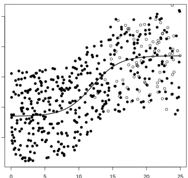
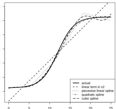
iidN(1,0.01). The scatterplot in Figure 1 shows the censoring mechanism for Configuration 1 and sample sizen= 500. Four different models were fitted to the data: one with linear term inx2 and three with spline terms of order 2, 3 and 4 (piecewise linear, quadratic and cubic) inx2. Knots at the quartiles of x2 were used in the spline models for Configuration 1, while for Configuration 2 two additional sets of knots for x2 were considered. In each case bootstrap confidence intervals were computed withb= 500 bootstrap replications.

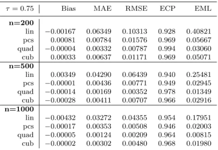
Tables 1 and 2 report average bias, median absolute error, root mean square error, empirical coverage probability (95% nominal coverage) and mean confi-dence interval length for the slope ofx1evaluated atτ = 0.50 and 0.75 (similar results were obtained for τ = 0.25) for Configuration 1. In all cases the par-tially linear model outperforms its linear equivalent. The difference between the three spline orders used is less clear, with some evidence that the quadratic spline works best. This is also supported by Figure 2, in which the quadratic spline term appears to give the best fit for the nonlinear term.

(9)

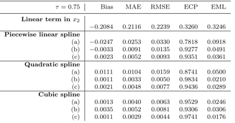
The effect of knot selection and placement is further investigated in the simulation study of Configuration 2, in which fitted spline models have knots at (a) the 33rd and 66th quantile of x2, (b) the quartiles of x2, and (c) the 20th, 40th, 60th and 80th quantiles ofx2. Tables 3 and 4 show the performance of various models fitted for Configuration 2. It is seen that again the spline models perform better than the linear model, while three knots are in general better than just two. The difference between three and four knots is less clear, as it appears that three knots are better for quadratic spline models, and four knots better for piecewise linear and cubic spline models.

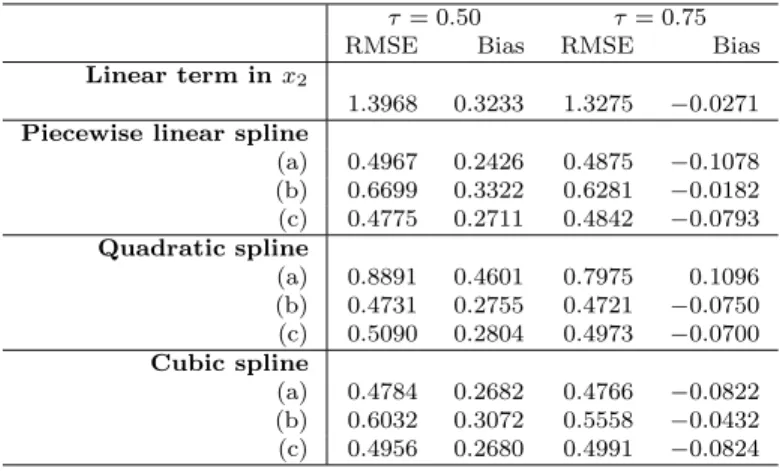
Finally, Table 5 reports bias and root mean square error for the estimation of the nonlinear term in Configuration 2. The quadratic spline with three knots appears to be performing better than other spline models in terms of root mean square error. Differences in bias are less obvious.

TABLES 1-5 ABOUT HERE.

5 Application to unemployment duration

We illustrate the usefulness of the partially linear CRQ model with an applica-tion to administrative unemployment data from the German Socio-Economic Panel Survey, a longitudinal survey of private households in Germany cover-ing topics such as income, employment, education and health. We focus on a subset of the data covering the period 1992-2004. The response variable of interest,Y, is the duration in months of the latest unemployment spell in the respondent’s work history.

We restrict our attention to males with German nationality (as both na-tionality and gender were found to be significant in preliminary analyses) and we explore the effect of age and marital status on unemployment duration. Exits from unemployment to full- or part-time employment were considered observed while all other exits were considered as censored observations. Ex-cluding observations with missing data, this gave a sample size of 2214 records with 55% censoring. Of these 2214 individuals, 42% were married. The median age for married respondents was 47.42 and for single 26.17.

The CRQ model

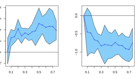
Qlog(Y)(τ|x) =β0(τ) +β1(τ)× married +θ(τ)⊤π(age) (8) was considered and quantiles up to the 60th were estimated. In particular, a quadratic spline term with knots at the quartiles of age was fitted. This provides a smooth 5-parameter fit to the age effect. All but one of the five coefficients were significant (at someτ-values), and so it is clear that the age effect requires more than a linear term.

Plots of ˆβ(τ), the estimated quantile coefficients for the intercept and mar-ital status, againstτare shown in Figure 3. The coefficients tend to be smaller in absolute value for short term unemployment (lowerτ values) and larger for long term unemployment (higherτ values).

(10)

Marriage has a strong negative effect on unemployment duration, indepen-dent of age (the relevant interaction terms were not significant). The estimated median coefficient representing the difference in log-duration between a sin-gle and a married German male is -0.8244 (confidence interval of (-1.1649,-0.4838)), i.e. median unemployment duration for a married respondent is 0.4385 times that of a single respondent of the same age. The size of the marriage effect is similar in all but the lowest quantiles of unemployment du-ration.

Plots of the estimated median unemployment duration against age are shown in Figure 4 separately for single and married German males. Pointwise bootstrap confidence intervals are also shown. The age ranges plotted reflect the different age distributions for married and single groups. For married males over 50, censoring exceeds 80%, thus we restrict attention for the married group to the “reliable estimation” age range (31.42,50.00) corresponding to the 10th age percentile and the age with 81% censoring above it. For single males the age range plotted is (19.67,47.17) corresponding to the 10th and 90th age percentiles. In the singles age distribution, 80% of the observations over age 47.17 are censored.

From Figure 4, it is clear that the age effect on unemployment duration is quite nonlinear (at least for single men), with age being beneficial at very low ages (<25) and rather detrimental (for both single and married men) at higher ages (as might be expected). The quantile analysis in Figure 5 presents perhaps a more surprising result. For quantiles belowτ = 0.3 (shorter unemployment durations), the effect is rather independent of age. This is not unexpected, as those who are readily re-employable do well at any age. However, for higher quantiles, the detrimental effect of age seems to increase rapidly for men in the range 30 - 50 years. The rather substantial increase in difficulty for older men who are not so readily re-employable would seem to call for some explanation (economic, psychological, or sociological).

Plots such as those in Figures 3-5 are useful in identifying departures from linearity. We advocate exploring the nonlinearity of each continuous covari-ate before attempting to fit linear coefficients as a way to detect patterns and improve the overall fit of the model. In addition, fitting a CRQ model is especially useful in highlighting population heterogeneity that is reflected in different structures for covariate effects for long and short durations. Such het-erogeneity can not be identified in general with proportional hazards models. While proportional hazards models with time-varying coefficients have been proposed (see Gray (1992) or Tian et al (2005) for a more recent example), such models focus on dynamic structural change and do not provide estimates of regression effects on specific population quantiles. That is, while such mod-els can identify secular trends, they can not identify structural variability for different population quantiles (as do CRQ models). It may be noted that such models are inherently nonparametric, even in the absence of partially linear covariate effects, with strictly slower convergence than the root-nasymptotics of standard regression quantile methods. On the other hand, time-varying co-variates or coefficients can not be incorporated directly into CRQ models (nor

(11)

into accelerated failure time models in general), and so CRQ models can not identify secular trends effectively.

6 Concluding remarks

In the preceding sections the use of a partially linear model for censored gression quantiles was proposed as a useful extension to standard linear re-gression techniques for survival data. The partially linear model was shown to be consistent and its use was illustrated by a data example and simulations. Quartile knots were used for the B-spline estimation of nonlinear terms and the quadratic spline gave satisfactory quantile estimates in the empirical example and simulations. Higher order spline terms did not show much improvement in estimation.

The censored regression quantile estimator is robust and flexible enough to highlight aspects of the data that the most common survival analysis tech-niques might overlook. Incorporating a nonlinear part adds even more flexi-bility to the model, allowing for more accurate estimation of parameters of interest, like quantile treatment effects. Censored regression quantiles and the semiparametric model proposed here are tools for capturing subtle aspects of the data and can be used in conjunction with other techniques for more comprehensive exploration of censored data.

The partially linear CRQ model can be extended to accommodate more than one nonlinear effects, as the basic theory extends directly to higher dimen-sions. However the curse of dimensionality could make application to two or more covariates quite problematic, in terms of slow convergence, complicated choice of a large number of knots, and interpretability.

As in every semiparametric model, the use of B-splines raises the question of knot selection. In this work the spline knots were chosen at fixed quantiles of the nonlinear variable. As long as the knot selection is not data-driven (e.g.equally spaced knots or quantile knots, perhaps depending on the sample size n), the asymptotic theory of B-splines applies directly (and consistency follows by Theorem 1 if the number of knots increases withn appropriately). Asymptotic results are not currently available if knot selection is data-driven. In practice fixing knots at specified quantiles of thex-variable is a simple and convenient solution for small to medium-sized datasets, and it is not likely that data-driven methods can offer much improvement here. However, in general it is also desirable to have a method for optimal knot selection and placement depending on the data. Such methods have been proposed by a number of authors. For instance, Koenker et al (1994) use a roughness penalty for quantile smoothing splines, and Doksum and Koo (2000) propose a method for stepwise knot addition and deletion using modified AIC and BIC for nonparametric quantile regression with regression splines. Further work along such lines would be useful for larger data sets.

(12)

Acknowledgments

This research was partially supported by National Science Foundation Grant DMS06-04229 and by the European Commission under the 6th Framework Programme’s Research Infrastructures Action (Trans-national Access contract RITA 026040) hosted by IRISS-C/I at CEPS/INSTEAD, Differdange (Lux-embourg). The data used in this publication were made available to us by the German Socio-Economic Panel Study (SOEP) at the German Institute for Economic Research (DIW), Berlin.

References

Buchinsky M, Hahn JY (1998) An alternative estimator for the censored quan-tile regression model. Econometrica 66:653–671

Chernozhukov V, Hong H (2002) Three-step censored quantile regression and extramarital affairs. J Am Stat Assoc 97:872–882

Doksum K, Koo J (2000) On spline estimators and prediction intervals in nonparametric regression. Comp Stat and Data Anal 35:67–82

Efron B (1967) The two-sample problem with censored data. In: Proceedings of the Fifth Berkeley Symposium, vol 4, pp 831–853

Gray RJ (1992) Flexible methods for analyzing survival data using splines, with applications to breast cancer prognosis. J Am Stat Assoc 87:942–950 He X, Shao Q (2000) On parameters of increasing dimensions. J Multivariate

Anal 73:120–135

He X, Shi P (1994) Convergence rate of B-spline estimators of nonparametric conditional quantile functions. Nonparametric Statistics 3:299–308

He X, Shi P (1996) Bivariate tensor-product B-splines in a partly linear model. J Multivariate Anal 58:162–181

Honore B, Khan S, Powell JL (2002) Quantile regression under random cen-soring. J Econometrics 109:67–105

Koenker R (2005) Quantile Regression. Cambridge University Press

Koenker R, Geling O (2001) Reappraising medfly longevity: a quantile regres-sion survival analysis. J Am Stat Assoc 96:458–468

Koenker R, Ng P, Portnoy S (1994) Quantile smoothing splines. Biometrika 81:673–680

Neocleous T, Vanden Branden K, Portnoy S (2006) Correction to:“Censored Regression Quantiles”. J Am Stat Assoc 101:860–861

Peng L, Huang Y (2008) Survival analysis with quantile regression models. J Am Stat Assoc 103:637–649

Portnoy S (2003) Censored regression quantiles. J Am Stat Assoc 98:1001– 1012

Portnoy S, Lin G (2008) Asymptotics for censored regression quantiles. Sub-mitted

(13)

Tian L, Zucker D, Wei LJ (2005) On the Cox model with time-varying regres-sion coefficients. J Am Stat Assoc 100:172–183

Vanden Branden K (2005) Robust methods for high-dimensional data, and a theoretical study of depth-related estimators. PhD thesis, Katholieke Uni-versiteit Leuven

Appendix: Proof of Theorem 1

The conditions for the main result (Theorem 1) are as follows: (I) Y andC are conditionally independent givenx

(F) For 0< ε <1, there exist constants aj, bj, cj withaj >0 andbj <∞for

uniformly forε≤FYi(y)≤1−ε,ε≤F˜Yi(u)≤1−εandε≤F˜Ci(v)≤1−ε and uniformly ini= 1, . . . , n. (X) max1≤i≤n||xi||=O(p). (XX) The matrix 1 n Pn i=1xix⊺i is positive definite.

Theorem 1 makes use of the theory of He and Shao (2000) on the asymp-totics of M-estimators when the parameter dimension increases withn. Briefly, this is outlined as follows. Let ˆβ_n ∈ Rm be the M-estimator for minimiz-ing Pn

i=1ζ(zi,β) for some data set{z1,z2, . . . ,zn} with zi ∈Rp+1 for i = 1,2, . . . , n; and for some objective kernel ζ(zi,β). If the objective function

is convex in β, and if ζ(z,β) is differentiable with respect to β, except at finitely many points, with derivative Ψ(z,β), then Theorem 2.1 of He and Shao (2000) states that under certain conditions, kβˆ_n −β∗k2 ₌ _O

p(m/n)

whereβ∗is the solution toPn

i=1EβΨ(zi,β) = 0. For the CRQ grid estimator

the increasing dimension ism=M p, whereM is the number of grid points. Let

p=O₍_nγ_{) for some}_{γ >}_{0. Equivalently,}_p_≤_cnγ _{for some constant}_c_{. Define}

Ψk(xi,β) =xi{∆i(I(Yi <x⊺iβ(tk))+(1−∆i)(wi(β, tk)I(Ci <x⊺iβ(tk))−tk)},

ηi(β′,β) =Ψ(xi,β′)−Ψ(xi,β)−E(Ψ(xi,β′)−Ψ(xi,β))

andSm={α∈Rm:kαk= 1}. Then

Ψ(xi,β) = (Ψ1(xi,β)⊺, Ψ2(xi,β)⊺, . . . , ΨM(xi,β)⊺)⊺∈Rm.

The result also relies on the following two lemmas, which have been shown in the case of fixedpby Vanden Branden (2005). Here the result is extended to the case of p growing with n. Lemma 1 permits restricting the proof to monotone functionsx⊺β(τ) on the grid. Lemma 2 shows thatτi(β) andτi(β∗)

(14)

Lemma 1 For everyB >0,∃ n0such that for n>n0 the set

β∈Rm:kβ−β∗k6Bm n

1/2

is contained in the set of all monotonic functions on the grid ε6 t1 < t2 <

. . . 6 tM 61−ε for some ε >0. Here tk−tk−1 =gn=n−κ,p≤cnγ for

somec >0, and m6p/gn, with γ≤ 1₂−3₂κ,κ >0.

Lemma 2 Let τi(β) be the gridpoint at which β crosses Ci, and let τi(β∗)

be the unknown gridpoint at which the true regression quantileβ∗ crosses the

same observation. It then holds that

|τi(β)−τi(β∗)|=O(T(n, m))

on the set{β:kβ−β∗k6B(m/n)1/2_}_with

T(n, m) = max(Bc1/2p1/2(m/n)1/2,2gn) = max(Bcnκ+γ−1/2,2n−κ).

Proofs of Lemmas 1 and 2 are straightforward generalizations of those in Vanden Branden (2005).

Proof (Proof of Theorem 1) It is sufficient to verify the following conditions

of He and Shao (2000). (C0) kPn

i=1Ψ(xi,βˆn)k=op(n1/2).

(C1) There exists aC andr∈(0,2] such that max i6n Eβ_θ sup :kθ−βk6d kηi(θ,β)k26nCdr for 0< d61. (C2) kPn i=1Ψ(xi,β∗)k=Op(nm)1/2 or Pni=1EkΨ(xi,β∗)k2=O(nm).

(C3) There exists a sequence of (m×m) matricesDnwith lim infn→∞λmin(Dn)>

0 (where λmin denotes the minimum eigenvalue) such that for anyB >0 and uniformly inα∈Sm sup kβ−β∗_k₆_B₍m n)1/2 |α⊺ n X i=1 E_β∗(Ψ(x_i,β)−Ψ(x_i,β∗))−nα⊺D_n(β−β∗)|=o(n1/2).

(C4) There exists a sequenceA(n, m) =o(n/logn) for which sup β:kβ−β∗k6B(m n)1/2 n X i=1 E_β|α⊺ηi(β,β∗)|2=O(A(n, m))

for anyα∈Sm, andB >0.

(C5) sup_α∈Smsupβ:kβ−β∗k6B(m n)1/2

Pn

i=1(α⊺ηi(β,β∗))2=Op(A(n, m)) for any

(15)

(C0) follows from the gradient conditions by noting that ||Ψ(ˆβ)||2=O_P₍_M _max 1≤k≤M||Ψk(ˆβ(tk))|| 2₎ and ||Ψk(ˆβ)||=OP( p plognmax||xi||). Thus ||Ψ(ˆβ)||=O_P₍_pp_M_log_n_{) =}O_P₍_nκ/2+γ_(log_n₎1/2₎_.

This isop(n1/2), provided thatκ/2 +γ <1/2.

For (C1), we note that had the xi been bounded by a constant, then

E_β||ηi,k(θ,β)||2would have been bounded by a constant also. Since max||xi||2=

O₍_p_{), then} _E_β_||η_i,k₍θ,β)||2 = O₍_p_{) and} _E_β_||η_i₍θ,β)||2 = O₍_{M p}_{), where}

M p≤cnκ+γ_{. Therefore one can take}_n _{large enough such that} _{C > κ}₊_γ _is

satisfied with 0< d≤1. For (C2), we note thatE||Ψk(β∗)||2=O(max||xi||2)

and n X i=1 M X k=1 E||Ψk(β∗)||2=O(M np) =O(mn).

(C3) and (C4) are the hardest conditions to prove. As shown in Vanden Bran-den (2005), forα∈Sm, α⊺E[Ψ(β)−Ψ(β∗)] =nα⊺Dn(β−β∗) (9) + n X i=1 M X k=1 α⊺_kxi n ˜ fY′i(u)(x ⊺ i(β(tk)−β∗(tk)))2 o (10) + n X i=1 M X k=1 α⊺_kxi ( _k X l=1 dklf˜C′i(v)(x ⊺ i(β(tl)−β∗(tl)))2 ) (11) where dkl =    −w1 l= 1 wk−1 l=k −(wl−wl−1) otherwise dkli= dkkf˜Ci(x ⊺ iβ ∗ (tk)) + ˜fYi(x⊺iβ ∗ (tk)) l=k dklf˜Ci(x⊺iβ∗(tl)) otherwise

(16)

and nDn =                n P i=1 d11ixix⊺i 0p,p . . . 0p,p n P i=1 d21ixix⊺i n P i=1 d22ixix⊺i . . . 0p,p · · · · n P i=1 dk1ixix⊺i n P i=1 dk2ixix⊺i . . . n P i=1 dkkixix⊺i 0p,p . . . 0p,p · · · · n P i=1 dM1ixix⊺i n P i=1 dM2ixix⊺i . . . . n P i=1 dMMixix⊺i                . (12) Thus for (C3) to hold we require

| n X i=1 M X k=1 α⊺_kxi ( ˜ fY′i(u)(x ⊺ i(β(tk)−β∗(tk)))2+ k X l=1 dklf˜C′i(v)(x ⊺ i(β(tl)−β∗(tl)))2 ) | =o(n1/2) (13)

or, as noted in Remark 2.3 of He and Shao (2000),

| n X i=1 M X k=1 α⊺_kxi ( ˜ fY′i(u)(x ⊺ i(β(tk)−β∗(tk)))2+ k X l=1 dklf˜C′i(v)(x ⊺ i(β(tl)−β∗(tl)))2 ) | =o((mn)1/2). (14) For( 10) we have n X i=1 M X k=1 α⊺_kxif˜Y′i(u)(x ⊺ i(β(tk)−β∗(tk)))2 ≤ n X i=1 M X k=1 |α⊺_kxi| M X k=1 (x⊺_i(β(tk)−β∗(tk)))2 ≤ n X i=1 ||xi|| M X k=1 ||αi||2 !1/2 ||xi||2 M X k=1 ||β(tk)−β∗(tk)||2 =O₍m n n X i=1 ||xi||3) =O(p3/2m) =O(n5γ/2+κ)

(17)

and for (11) n X i=1 M X k=1 α⊺_kxi k X l=1 dklf˜C′i(v)(x ⊺ i(β(tl)−β ∗₍_t l)))2 ≤ n X i=1 M X k=1 α_k⊺xidk1f˜C′i(v)(x ⊺ i(β(tl)−β∗(tl)))2 (15) + n X i=1 M X k=1 α⊺_kxi k X l=2 dklf˜C′i(v)(x ⊺ i(β(tl)−β∗(tl)))2 (16)

Noting thatdkl =O(1) forl= 1 andO(M) otherwise, we obtain

(15)≤ n X i=1 M X k=1 ||α⊺_kxi||2 !1/2 _M X k=1 d2 k1 !1/2 ||xi||2||β(t1)−β∗(t1)||2 ≤ n X i=1 ||xi||3M1/2||β(t1)−β∗(t1)||2=O(p3/2M1/2 m n) =O(n5γ/2+3κ/2) and (16)≤ n X i=1 M X k=1 α⊺_kxi k X l=2 d2kl !1/2 _k X l=2 (x⊺_i(β(tl)−β∗(tl)))2 ≤ n X i=1 M X k=1 α⊺_kxi _k₋₁ M2 1/2 ||xi||2 k X l=2 (β(tl)−β∗(tl))2 =O₍_M1/2m n n X i=1 ||xi||3) =O(p3/2M1/2 m n) =O₍_n5γ/2+3κ/2₎_.

With γ and κ satisfying 2γ+κ < 1/2, the error from (C3) can be made

o((mn)1/2_{) =}_o₍_nγ/2+κ/2+1/2_).

(C4) needs to hold with A(n, m) =o(n/logn). The term α⊺_η

i(β,β∗) is defined as α⊺ηi(β,β∗) = M X k=1 α⊺_k(Ψk(xi,β)−Ψk(xi,β∗)−E(Ψk(xi,β)−Ψk(xi,β∗))). (17) A Taylor series expansion for the expectation part of the expression gives

M X k=1 α⊺_kxi " ˜ fYi(u)(x⊺i(β(tk)−β∗(tk))) + k X l=1 dklf˜Ci(v)(x⊺i(β(tl)−β∗(tl))) #

(18)

for someuandv. Similarly as for (C3) the first part of this term is bounded by O₍₍_m/n₎1/2_p_{) =} O₍_nκ/2+3γ/2−1/2_{) and the second part is bounded by} O₍_p₍_{M m/n}₎1/2_{) =}O₍_n3γ/2+κ/2−1/2_{). Therefore} α⊺ηi(β,β∗) = M X k=1 α⊺_k(Ψk(xi,β)−Ψk(xi,β∗)) +O(n3γ/2+κ/2−1/2).

This error term squared and multiplied bynisO₍_n3γ+κ_{) which can be made}

o(n/logn) if 3γ+κ <1 so that it satisfies the requirement for (C4). For the term inPM

k=1α ⊺

k(Ψk(xi,β)−Ψk(xi,β∗)) we introduce an indicator,Iak,bk(Y), withIak,bk(Y) =±1 ifY lies in betweenx

⊺

ia(tk) andx⊺ib(tk), and 0 otherwise.

Then M X k=1 α⊺_k(Ψki(β)−Ψki(β∗)) = M X k=1 α⊺_kxisign (x⊺i(β(tk)−β∗(tk))× [I(Yi6Ci)I_β k,β ∗ k(Yi) +I(Yi> Ci)w(β ∗_{, t} k)I_β k,β ∗ k(Ci)] + M X k=1 α⊺_kxiI(Yi> Ci)I(Ci6x⊺_iβ(tk))(wi(β, tk)−wi(β∗, tk)).

The last term can be bounded using Lemma 2. For some constantD |wi(β, tk)−wi(β∗, tk)|= (tk−1)(τi(β)−τi(β∗)) (1−τi(β))(1−τi(β∗)) 6DT(n, m) where T(n, m) is as defined in Lemma 2. Therefore the last term can be bounded by

O₍_M1/2_p1/2_T₍_{n, m}_{)) = max} O₍_M1/2_p₍_m/n₎1/2₎_,O₍_p1/2_/M1/2₎

= max(O₍_n3γ/2+κ−1/2₎_,O₍_nγ/2−κ/2₎₎_.

Combining these results gives

|α⊺ηi(β,β∗)|6 M X k=1 {|α⊺_kxi|[|I(Yi6Ci)I_β k,β ∗ k(Yi)|+|I(Yi> Ci)Iβk,β ∗ k(Ci)|}] + maxO₍_n3γ/2+κ−1/2₎_,O₍_nγ/2−κ/2₎_.

This error term squared and multiplied bynwill beo(n/logn) if 3γ+ 2κ <1 andγ−κ <0.

Finally for the term

M X k=1 {|α⊺_kxi|[|I(Yi6Ci)I_β k,β ∗ k(Yi)|+|I(Yi> Ci)Iβk,β ∗ k(Ci)|}] !2 ,

a bound is required on the number of observations for which I_β

k,β ∗ k(Yi) and I_β l,β ∗

(19)

bounded byD∗_T₍_{n, m}₎_M _{for some constant}_D∗_{. A bound of}_O₍_p₍_m/n₎1/2_{) =}

O₍_n3γ/2+κ/2−1/2_{) is thus obtained for the main part of the square. The cross}

term contributes

O₍_p₍_m/n₎1/2_T₍_{n, m}₎_M_{) = max} O₍_n5γ/2+5κ/2−1₎_,O₍_n3γ/2+κ/2−1/2₎

.

The contribution of both terms can once again be madeo(n/logn) if 5γ/2 + 5κ/2<1 and 3γ/2 +κ/2<1/2.

The constraints onκandγyield equations (5), (6) and (7). All that is left is to verify that (C5) holds for these values.

According to Lemma 2.2 of He and Shao (2000), (C5) holds with the same

A(n, m) as in (C4), provided thatc2

n,mmlogn=O(A(n, m)), where cn,mis a

sequence satisfying sup_β_,_xkΨ(x,β)k 6cn,m. Here cn,m =D∗∗M1/2p1/2 for

some constant D∗∗_{. Recalling that} _p₌ _O₍_nγ_{), it follows that} _c2

n,mmlogn =

O₍_A₍_{n, m}_{)), which concludes the proof of Theorem 1.}

Remark. The results obtained in Theorem 1 are not optimal. For example, one possible choice for γ and κis γ = 1/7 and κ = 1/5 which would give a rate of order n−23/35_{. In addition, if condition (C4) holds with} _A₍_{n, m}_{) =} o( n

mlogn), Theorem 2.2 of He and Shao (2000) gives asymptotic normality

of the estimator, but requires tighter bounds than those obtained in Vanden Branden (2005), Neocleous et al (2006) and in Theorem 1. That is not to say that asymptotic normality is not possible. In fact, empirical results show that as the sample sizenincreases, the distribution of the CRQ-estimated βˆ

(20)

Table 1 Comparison of performance forβ1(0.50) in the simulation model with approximate

20% censoring (Configuration 1). Knots at the quartiles of x2 were used for the spline

terms. The average bias, median absolute error, root mean square error, empirical coverage probability (95% nominal coverage) and mean confidence interval length are shown.

τ= 0.50 Bias MAE RMSE ECP EML

n=200 lin −0.00188 0.07646 0.11086 0.940 0.45406 pcs −0.00012 0.00413 0.01115 0.996 0.04806 quad 0.00033 0.00436 0.00997 0.980 0.03552 cub 0.00024 0.00831 0.01420 0.968 0.05564 n=500 lin 0.00262 0.05208 0.07554 0.936 0.28953 pcs 0.00003 0.00216 0.00419 0.990 0.01669 quad −0.00019 0.00228 0.00452 0.950 0.01692 cub −0.00003 0.00573 0.00843 0.960 0.03405 n=1000 lin −0.00198 0.03420 0.04850 0.952 0.20286 pcs 0.00001 0.00124 0.00228 0.982 0.00934 quad −0.00011 0.00158 0.00291 0.950 0.01088 cub −0.00005 0.00420 0.00609 0.954 0.02488

Table 2 Comparison of performance forβ1(0.75) in the simulation model with approximate

20% censoring (Configuration 1). Knots at the quartiles of x2 were used for the spline

n=200 lin −0.00167 0.06349 0.10313 0.928 0.40821 pcs 0.00081 0.00784 0.01576 0.969 0.05667 quad −0.00004 0.00332 0.00787 0.994 0.03060 cub 0.00033 0.00637 0.01171 0.969 0.05071 n=500 lin 0.00349 0.04290 0.06439 0.940 0.25481 pcs −0.00001 0.00436 0.00771 0.949 0.02945 quad −0.00014 0.00169 0.00352 0.978 0.01349 cub −0.00028 0.00411 0.00707 0.966 0.02916 n=1000 lin −0.00432 0.03272 0.04355 0.954 0.17951 pcs −0.00017 0.00353 0.00508 0.946 0.02003 quad −0.00005 0.00124 0.00209 0.964 0.00815 cub −0.00002 0.00302 0.00480 0.968 0.01980

(21)

Table 3 Comparison of performance forβ1(0.50) in the simulation model withn= 500 and

approximate 40% censoring (Configuration 2). Knots at (a) the 33rd and 66th quantiles, (b) the quartiles and (c) the 20th, 40th, 60th and 80th quantiles ofx2 were used for the spline

Linear term inx2

−0.1074 0.1069 0.1256 0.6640 0.2835

Piecewise linear spline

(a) −0.0166 0.0173 0.0233 0.7980 0.0645 (b) 0.0108 0.0109 0.0212 0.9457 0.0641 (c) 0.0056 0.0081 0.0144 0.9618 0.0526 Quadratic spline (a) 0.0276 0.0288 0.0348 0.7560 0.0917 (b) 0.0010 0.0032 0.0055 0.9739 0.0219 (c) 0.0030 0.0047 0.0081 0.9379 0.0279 Cubic spline (a) 0.0018 0.0038 0.0060 0.9700 0.0242 (b) 0.0061 0.0080 0.0110 0.9280 0.0379 (c) 0.0008 0.0026 0.0040 0.9699 0.0172

Table 4 Comparison of performance forβ1(0.75) in the simulation model withn= 500 and

approximate 40% censoring (Configuration 2). Knots at (a) the 33rd and 66th quantiles, (b) the quartiles and (c) the 20th, 40th, 60th and 80th quantiles ofx2 were used for the spline

Linear term inx2

−0.2084 0.2116 0.2239 0.3260 0.3246

(a) −0.0247 0.0253 0.0330 0.7818 0.0918 (b) −0.0033 0.0091 0.0135 0.9277 0.0491 (c) 0.0023 0.0052 0.0093 0.9351 0.0361 Quadratic spline (a) 0.0111 0.0104 0.0159 0.8741 0.0500 (b) 0.0011 0.0033 0.0050 0.9834 0.0210 (c) 0.0021 0.0048 0.0077 0.9436 0.0289 Cubic spline (a) 0.0013 0.0040 0.0063 0.9529 0.0246 (b) 0.0035 0.0052 0.0081 0.9306 0.0306 (c) 0.0011 0.0029 0.0044 0.9741 0.0176

(22)

Table 5 Comparison of performance forQ(τ |x) in the simulation model withn= 500 and approximate 40% censoring (Configuration 2). Knots at (a) the 33rd and 66th quantiles, (b) the quartiles and (c) the 20th, 40th, 60th and 80th quantiles of x2 were used for the

spline terms. The root mean square error and average bias are shown for the 50th and 75th conditional quantiles evaluated at the mean ofx1.

τ= 0.50 τ= 0.75

RMSE Bias RMSE Bias

Linear term inx2

1.3968 0.3233 1.3275 −0.0271

(a) 0.4967 0.2426 0.4875 −0.1078 (b) 0.6699 0.3322 0.6281 −0.0182 (c) 0.4775 0.2711 0.4842 −0.0793 Quadratic spline (a) 0.8891 0.4601 0.7975 0.1096 (b) 0.4731 0.2755 0.4721 −0.0750 (c) 0.5090 0.2804 0.4973 −0.0700 Cubic spline (a) 0.4784 0.2682 0.4766 −0.0822 (b) 0.6032 0.3072 0.5558 −0.0432 (c) 0.4956 0.2680 0.4991 −0.0824

(23)

0 5 10 15 20 25 5 10 15 20 25 x2 y

Fig. 1 Scatterplot of Configuration 1 used in the simulation experiment. Censored points are shown as open circles, uncensored points as filled circles. The conditional median line evaluated at the mean ofx1is also shown.

(24)

0 5 10 15 20 25 8 10 12 14 16 18 20 x2 y actual linear term in x2 piecewise linear spline quadratic spline cubic spline

Fig. 2 Various model fits for the nonlinear term in the simulation experiment (Configuration 1). Shown here are the actual median (solid line) and model-estimated conditional median lines (dashed or dotted) evaluated at the mean ofx1.

(25)

0.1 0.3 0.5 0.7 −2 0 2 4 6 8 (Intercept) o o o o o o o o o o o o o o o 0.1 0.3 0.5 0.7 −1.0 −0.5 0.0 married o o _o o o o o o o o o o o _o o

Fig. 3 Estimated linear coefficients ˆβ0(τ) and ˆβ1(τ) in model (8) with 95% bootstrap

pointwise confidence intervals plotted againstτfor 0< τ≤0.75.

35 40 45 50 4 6 8 10 12 14 16 Age (years)

Unmeployment duration (months)

Married 20 25 30 35 40 45 4 6 8 10 12 14 16 Age (years)

Unemployment duration (months)

Single

Fig. 4 Estimated median unemployment duration against age for German males. The black line shows the median, grey lines show 95% pointwise confidence limits.

(26)

35 40 45 50 0 5 10 15 Age (years)

Married 20 25 30 35 40 45 0 5 10 15 Age (years)

Single

Fig. 5 Estimated deciles of unemployment duration against age for German males. The solid line shows the median, dashed lines show the other deciles from 1st to 6th.