Short-Term Forecasting of Wind Speed and Wind Power Based on BP and Adaboost_BP

Theses and Dissertations

August 2014

Short-Term Forecasting of Wind Speed and Wind

Power Based on BP and Adaboost_BP

Sibei Mi

University of Wisconsin-Milwaukee

Follow this and additional works at:https://dc.uwm.edu/etd Part of theElectrical and Electronics Commons

This Thesis is brought to you for free and open access by UWM Digital Commons. It has been accepted for inclusion in Theses and Dissertations by an authorized administrator of UWM Digital Commons. For more information, please contactopen-access@uwm.edu.

Recommended Citation

Mi, Sibei, "Short-Term Forecasting of Wind Speed and Wind Power Based on BP and Adaboost_BP" (2014).Theses and Dissertations. 505.

WIND POWER BASED ON BP AND ADABOOST_BP

by

Sibei Mi

A Thesis Submitted in

Partial Fulfillment of the

Requirements for the Degree of

Master of Science

in Engineering

at

The University of Wisconsin-Milwaukee

August 2014

ii

SHORT-TERM FORECASTING OF WIND SPEED AND WIND

POWER BASED ON BP AND ADABOOST_BP

by

Sibei Mi

The University of Wisconsin-Milwaukee, 2014

Under the Supervision of Professor David C. Yu

Due to wind is intermittent and less dispatchable, wind power fluctuates as the

wind fluctuating and is uncontrollable. Therefore, when wind power accounts

for a higher proportion of total electricity generation of the system, power

generation plan needs to arrange according to the variation of wind power

output. The way to solve the problem is forecasting the wind power.

In this paper, we focus on the wind speed and wind power forecasting in the

time scales of 10min, 1h and 3h in the future. BP Neural Network and

Adaboost_BP Neural Network are selected as the forecasting model for wind

speed forecasting. And for wind power forecasting model, we use BP Neural

iii

turbines in the same type. As the geographical distribution of this wind farm is

unknown, we pick one No.17 wind turbine as the optimal one by analyzing the

data of 31 wind turbines and making the curve fitting of wind speed and wind

power. Then we analyze the influencing factor of wind power, and find out

wind speed as the most influential factor. For the wind speed, we deal with the

raw data which selected from SCADA (Supervisory Control and Data

Acquisition) system before using it.

For the wind speed forecasting model, we find the optimal number of the

training data for each training sets for the BP Neural Network in each time

scale. Then we make a contrast of the accuracy of the single-step forecasting

accuracy between BP Neural Network model and Adaboost_BP model in

10min, 1h and 3h at their respectively optimal number of the training data. And

there is a comparison between the accuracy of the single-step and iterative

multi-step wind speed forecasting model in 1h and 3h time scales at the number

iv

its corresponding wind power to build the input matrix for the network training.

And we find that not only the number of the training data for each training sets

but also the range of wind power affects the forecasting accuracy. Then make a

contrast of the wind power forecasting result with forecasting wind speed and

vi

LIST OF FIGURES ... viii

LIST OF TABLES ... ix

Acknowledgements ... x

I. INTRODUCTION ... 1

1.1. Introduction ... 1

1.2. Wind Power Forecasting Methods ... 4

A. Classification of Wind Power Forecasting Methods ... 4

B. Physical Models of Wind Power Forecasting Methods ... 6

C. Time Sequence Models of Wind Power Forecasting Methods ... 8

D. Artificial Intelligence Models and Other Models of Wind Power Forecasting ... 9

II. DATA PROCESSING ... 11

2.1. Wind Turbine Selection ... 11

A. Data Normalization ... 11

B. Eliminate the Zero Point of Wind Power ... 12

C. Order of Carving Fitting ... 13

D. Select the Wind Turbine ... 15

2.2. Influencing Factors of Wind Power ... 17

2.2.1 Air Density ... 18

2.2.2 Wind Direction ... 18

2.2.3 Wind Speed ... 19

III. WIND SPEED FORECASTING ... 23

3.1. Introduction ... 23

3.2. The Basic Principle of Artificial Neural Network ... 23

3.2.1 Neuron Model ... 25

3.2.2 Commonly Used Transfer Function ... 26

3.2.3 Neural Network Structure ... 29

vii

3.3.2 The Short-term Wind Speed Forecasting Based on BP Neural Network

Learning Algorithm ... 34

3.4. Adaboost ... 45

3.4.1 Adaboost Algorithm Overview ... 45

3.4.2 BP Neural Network Algorithm Based on Adaboost ... 47

IV. WIND POWER FORECASTING ... 51

4.1. Introduction ... 51

4.2. Wind Power Forecasting Model ... 51

4.2.1 Input matrix ... 51

4.2.2 The Range of Wind Power ... 53

4.2.3 The Wind Power Forecasting ... 56

V. CONCLUSION ... 59

viii

Figure II-1 5th-order Carving Fitting without Eliminating the Zero Points ______________________ 13 Figure II-2. Carving Fitting ___________________________________________________________ 14 Figure II-3. Carving Fitting ___________________________________________________________ 15 Figure II-4. Crave Fitting of No.17 in March 2011 _________________________________________ 16 Figure II-5. Bad Data Replacement _____________________________________________________ 21 Figure III-1. Commonly Used Transfer Functions _________________________________________ 27 Figure III-2. BP Neural Network _______________________________________________________ 32 Figure III-3. BP Neural Network Learning Steps __________________________________________ 34 Figure III-4. BP Neural Network Model in Matlab _________________________________________ 35 Figure III-5 Adaboost Algorithm _______________________________________________________ 46 Figure III-6. Adaboost_BP Neural Network Learning Steps _________________________________ 48 Figure IV-1 Wind Speed Distribution of Wind Turbine No.17. _______________________________ 55 Figure IV-2 Forecasting Range of Wind Speed and Wind Power ______________________________ 56

ix

Table II-1 Low Wind Speed and Its Corresponding Wind Power ______________________________ 13 Table II-2 RMS of Error of Wind Turbine ________________________________________________ 16 Table II-3 Example of Training Matrix __________________________________________________ 21 Table III-1 Element of Multi-step Wind Speed Forecasting Matrix __________________________ 41 Table III-2. Single-step and Iterative Multi-step Wind Speed Forecasting Model __________________ 42 Table III-3. Number of Training Data for Each Training Sets for 10min ________________________ 43 Table III-4. Number of Training Data for Each Training Sets for 1h ___________________________ 44 Table III-5. Number of Training Data for Each Training Sets for 3h ___________________________ 44 Table III-6 Wind Dpeed Forecasting Result of BP and AdaBoost_BP ________________________ 49 Table III-7 Wind Speed Forecasting of Single-step and Iterative Multi-step Model _______________ 50 Table IV-1 Number of Training Data for Each Training Sets _________________________________ 53 Table IV-2 Wind Power Forecasting in Different Wind Power Range ________________________ 54 Table IV-3 Wind Power Forecasting ____________________________________________________ 57

x

This thesis wouldn't have been possible without the help and support of

several people.

I would like to express my deep and sincere gratitude to my supervisor

Prof. David C. Yu. With his invaluable support, guidance and patience, I

make this thesis possible. He built up the communicational bridge

between

the

universities

in

China

and

the

University

of

Wisconsin-Milwaukee, and this gave me the opportunity to come to

United States for further study.

I am grateful to Xiaoxuan Lou and Zhenze Long. Their insightful

comments helped me to improve this thesis.

Last but not least, I would like to thank my family, my mother Yanxi

Zhou, my father Ge Mi and my aunt Xiaoling Mi, for their unconditional

love and support they have shown me throughout my life.

I.

INTRODUCTION

1.1.

Introduction

Electricity can be generated by a variety of ways. Apart from solar photovoltaic power generation, other forms of electricity generation are in the same way that primary energy pushes prime mover, and then the prime mover drives generators to generate electricity. Wind power has many characteristics which other fossil energy does not have, such as clean, intermittent and randomness. This is because the wind is a natural phenomenon. Wind energy converts into mechanical energy in the way that wind blow through fans to drive rotor rotation. And then the energy converts into electricity without generating pollution and radiation which will be generated in the electricity conversion process of conventional energy. The reason why the demand for wind power around the world grows involves many aspects, including the shortage of energy, change in climate, the progress of economy and technology, etc.

In 2006, International Energy Agency pointed out the world's energy demand would be 60% higher than in that year, and the supply of fossil fuels would be reduced [1]. The energy in some countries would be relied on imports, and this would affect the stability of geopolitics in these countries. On the contrary, as a new energy without energy costs, wind energy exists in various countries and regions all over the world. Therefore the use of wind power as a new energy will become an important strategy for the world to solve the problem of energy crisis.

Besides, another impetus for the rapid development of wind power is the increasingly serious problem of global climate change which is known as the most seriously worldwide recognized environmental threat. In the 1997 Kyoto protocol, developed countries reached an agreement to decrease the totality of the emissions of six kinds of greenhouse gas at least 5% from 1990 levels in 2008-2010 (8% for Europe, 7% for United States and 6% for Canada). In addition, the development of nuclear energyis constrained by concerning about the radioactive waste. Especially the leakage of nuclear materials of Japan Fukushima nuclear power plant in March 2011 made countries around the world to reconsider their nuclear policies. Nuclear power development in China has therefore been put off, while Germany will shut down all nuclear power plants by 2022. Thus, the declination of the status of nuclear power in clean energy makes the development of other clean energy like wind power more urgent.

In the 1880’s, with the development of the global wind power market, sharp decline in the price of wind power equipment made contribution to the development of wind power industry. In the area which is rich in wind resources, the cost of electricity generation of wind power is not expensive which can be competitive with that of coal and natural gas. And with the increase in the price of fossil fuels in recent years, the competitiveness of wind power gets greatly improved. Besides, considering the extra charges and the impact on people's health as parts of generating cost which caused by the pollution from fossil fuels and nuclear radiation, the price of wind power is more competitive [2].

In recent years, the rapid development of wind power industry is mainly driven by national policy, environment and economy. And the development of wind turbine technology plays an essential role. Since the first commercial wind turbine launched in the 1880’s, the capacity, efficiency and the visual design of wind turbines have been greatly improved. The modern wind turbines are modularity and easy to install. The capacity of wind farm Increased from a few MW to several hundred MW.

According to the report from global wind energy council, the growth rate of the wind power are faster than that of other renewable energy sources in the past ten years. Starting in 2000, the annual average growth rate of installed wind energy capacity reaches 28%. And it is estimated that the global installed wind energy capacity will be 233-486GW by 2015 and reach 352-1081GW by 2020.

Compared with traditional fossil fuel power plants, the electricity production in wind power plants is quite different. The most different one is the production of wind power depends on the existence of the wind which is an uncontrollable natural phenomenon [3]. However, the generating capacity of both traditional fossil fuel power plants and nuclear power plants can be controlled according to the load demand. But, due to wind is intermittent and less dispatchable, wind power also fluctuates as the wind fluctuating and is uncontrollable. When the power system operates, the output of electricity and the load must be equal at any time. Therefore, when wind power accounts for a higher proportion of total electricity generation of the system, power generation plan needs to arrange according to the variation of wind power output.

Wind power forecasting is an important way to solve this challenge. Under the conventional power generation way, power system operation needs to forecast the load and develops electricity generation schedule for traditional power plants. However, after adding wind power to the system, the wind speed and power forecasting is needed in order to make wind power in the electricity system scheduling plan. Unlike the traditional electricity generation schedule, the accuracy of the wind speed and power forecasting is far less than that of load forecasting for its uncontrollability. Hence, it is important to reserve more spinning reserve or add another energy storage device while making the electricity system scheduling plan.

1.2.

Wind Power Forecasting Methods

A. Classification of Wind Power Forecasting Methods

Wind speed and wind power forecasting have been developed over 30 years. A number of wind speed and wind power forecasting models for commercial and research use are made in recent years. In countries such as Denmark, Germany and Spain, Wind power occupies a large proportion in the whole power system, and wind power forecasting system has become an important part of power and control system. Wind power forecasting model is divided into statistical model, physical model and the combination of the two models according to the input data [4]. In general, different forecasting models require different inputs. Considering the most important influence factor of wind farm output power is the local wind speed, wind speed is the

essential input for all forecasting model. The data types of inputs which can be used for predictive models include Numerical Whether Predictions, online data of wind farm, physical environment data (including topography, surface roughness and the distribution of wind farm, etc.) and user information [5]. For the statistical model, it only need the online measurement data of wind farm, such as the wind farm output power, the power output of a single wind turbine and meteorological data (wind speed and direction, etc.). And it also can use the meteorological information provided by the Numerical Weather Prediction (NWP) [4]. As for the physical model, it mainly depends on the numerical weather prediction (NWP), and use some physical conditions of geography, such as surface features (topography and roughness and obstacles), and the technical information of the wind turbine (for example, the center height, power curve and penetrating power) [4,6,7]. Combination of the two forecasting models can have the high accuracy in a relatively short time which comes from the statistical model as well as the longer time scale forecasting of the physical model.

Wind power forecasting model also can be classified according to the forecast time length, and the forecast time length depends on the application purpose of forecasting model and the technology it uses. For instance, the forecast result which the forecast time length is a few seconds to a few minutes can be used for the dynamic control of the wind turbine system [5,8], and the forecast result which the forecast time length is one hour or a few hours can be used for the safe operation and the economic dispatch of the power system [4, 9]. Classifying by the forecasting technique is another way for

the classification of wind power forecasting model. The forecasting model can be divided in physical model, time sequence model, artificial intelligence model and spatial correlation model, etc.

B. Physical Models of Wind Power Forecasting Methods

Currently, the forecast time length of physical model can be up to 48 hours. These models mainly depend on the numerical weather prediction (NWP), and need to take some other physical factors into consideration, such as the local surface roughness, the influence of terrain and obstacles, the layout of wind farm and the wind turbine power curve [4,6,7]. The physical model has higher forecast accuracy for a long forecast time length. However, it is very complex and expensive to make forecasting by using physical models. Besides, for the short-term forecasting (a few hours forecasting), the forecasting results are often not satisfactory as the delay of data updating [7]. Generally physical models are used as the first step of the wind speed forecasting, and its forecasting results will be the input of other statistical models. Nowadays, there are multiple physical models which can be used for wind power forecasting. One of them is high-resolution limited area model (HIRLAM) which established in 1999 by Landberg [10]. The model uses the Numerical weather forecasting data which is provided by HIRLAM as the input. The research of numerical weather forecasting data is in a long-term scale forecasting in power plants. The collecting data of wind farm must be related to a rough model which considers the influences of local territory, and use WASP mode for local wind speed forecasting

by taking the local impact into account. In order to solve the effect of the wake flow of wind turbines, PARK scheme is adopted. The fan chart is presented in PARK which declares the reduce of wind farm output power due to the wake flow of wind turbines. Then obtain the wind farm output power which calculates from the model output data. The model is successfully applied to multiple wind farms in Denmark. The model runs twice a day and provides the forecasting for 36 hours in advance. Compared with continuous model, the forecasting results of this model is better than that of the continuous model when forecasts for more than 4 hours.

In the reference [11], Focken studied the influence of the decrease of the wind power forecasting error due to the spatial smoothness. The model used the NWP data provided by Deutscher Wetterdienst, including the forecasting data for 6, 12, 18, 24, 36 and 48 hours in advance. The forecasting model provides the wind farm output power forecasting for 48 hours in advance. In this model, the wind speed of the center height of wind turbines is calculated by the formula of wind profile. In addition, the model also considers the differential thermal of the boundary layer, the surface roughness and terrain of wind farms and the wake effect of wind turbines. Using the statistical model as the forecasting method for wind farm power output, the final output of the model is an output power of a wind farm. Compared the average error of wind power forecasting in 30 wind farms in Germany with that of a single wind farm, the forecasting precision of the spatial correlation model is higher than that of a single address model. The reason is the influence of spatial smoothing effect, and the improvement of the forecasting precision depends on the size of the region and the

number of wind farms in the region.

C. Time Sequence Models of Wind Power Forecasting Methods

At present, several time sequence models have been put forward which can be used for wind speed and wind power forecasting, such as AR model, MA model, ARMA model, ARIMA model, time sequence model based on neural network and gray model etc. The characteristics of time sequence models are simple and easy to modeling, and the input data of the model only need to be wind speed and wind power in the past. However, the accuracy of time sequence forecasting model as will have fallen sharply as the increase of the length of the forecasting time. Therefore, these time sequence models usually used to forecast short-term wind speed and wind power.

Sfetsos (2002) used the auto-regressive integrated moving average (ARIMA) model and the feed forward neural network as the forecasting model, and put forward the wind speed forecasting model an hour in advance based on the two different time sequence models in the reference [12]. One forecasting model used the average wind speed in an hour to make one step forecasting in advance. The other one used the average wind speed in 10 min to make six steps forecasting to get wind speed forecasting data an hour in advance. Comparing the two forecasting methods with the persistence approach, the prediction accuracy of Artificial Neural Network (ANN) model is higher than that of the persistence approach. However, the prediction accuracy of ARIMA model is higher than that of ANN model.

Huang and Chalabi (1998) presented an auto-regression (AR) model which could use to forecast wind speed an hour or several hours in advance in the reference [6]. This

algorithm considered the unstable characteristics of wind speed and used Kalman filter to estimate the time variation parameter of AR model.

Erasmo and Wilfrido (2007) used ARIMA model and ANN model to make a monthly time-step size wind speed forecasting with the wind speed data for past 7 years in advance in the reference [13]. And comparing this method with the persistence approach, ARIMA model has a higher prediction accuracy for wind speed. EI-Fouly (2006) presented the gray model (GM(1,1)) to forecast wind speed for an hour in advance in the reference [14]. The wind speed forecasting data which is provided by GM(1,1) model is used to forecast wind power as the input of the 600kW wind turbine power formula. Comparing the forecasting result of GM(1,1) model with that of the persistence approach, the forecasting accuracy of wind speed was improved about 11.2% than the persistence approach method and the forecasting accuracy of wind power is increased by about 12.2%.

EI-Fouly (2006) put forward a time sequence model for wind speed forecasting which could carry out the wind speed 24 hours in advance [5]. In this model, the data came from three times of three years data set of a meteorological station. And compared this method with the persistence approach, this model has a better forecasting result while the forecasting time length is 3, 6, 12 and 24 hours.

D. Artificial Intelligence Models and Other Models of Wind Power Forecasting

In recent years, the artificial intelligence method，such as artificial neural network, fuzzy logic and hybrid model, has been widely used. As the artificial intelligence

method can simulate nonlinear problems very well, many researchers found that the wind speed and wind power forecasting can get good result by using these methods. Shuang (2007) used Tabu Search Algorithm optimized the link weight of BP neural network, and forecasted the wind speed 1 hour in advance by using this model [15]. The number of input neurons was decided by correlation analysis. Thus, ANN model could learn better in this way. The result showed that ANN model which used the new training method has a better accuracy in wind speed forecasting than traditional BP neural network model.

Leigh and Ran (2008) decomposed the wind speed time series which is highly nonlinear into several relatively stable time series. Every time series is decomposed from the original wind speed sequence according to the different resolution. And ARMA model forecasting models are established for every time series to forecast the next value of this series, then use the combination method of the forecasting data to synthetize the forecasting wind speed 1 hour in advance. The actual mean hourly wind speed used in this article to establish the forecasting model came from meteorological station. Compared this method with the continuous approach and the original ARMA method, this model improved the forecasting accuracy.

Senjyu (2006) presented a feedback neural network (RNN) to forecast the wind speed 3 hours to 3days in advance by time series method [16]. Compared this method with feed forward neural network (FNN), RNN method can reduce the forecasting error and improve the forecasting effect of wind speed and wind power.

II.

DATA PROCESSING

At present, the common method used for wind power forecasting is using neural network to establish the corresponding forecasting model of the forecast data and wind power, and the forecasting data is the meteorological forecasting data of the wind tower which is near the wind farm. In order to use the neural network to establish the model, the most essential step is selecting the appropriate network input variables by analyzing the influence factors of wind turbine power output. Then the data used in the forecast is the processed one of the raw data.

2.1.

Wind Turbine Selection

The wind farm which the data used in this paper comes from has 31 wind turbines in the same type. While the geographical distribution of this wind farm is unknown, one wind turbine is picked out from the wind farm in this paper. By analyzing the data of 31 wind turbines and making the curve fitting of wind speeds and wind powers, No.17 wind turbine has been found out as the optimal one. The steps are:

A. Data Normalization

Due to the data ranges of variables are different and the values may vary widely, large numerical variables have bigger influence on the results when establish mathematical model to solve problems. If one small numerical variable had a great influence on the result, it might play a small role in building the mathematical model. In order to avoid such a situation, the data which is used in modeling need to be normalized first.

Normalization can transform the value of variables into a specified range, usually [-1, 1] or [0, 1].

Considering the range of wind speed is 0-30m/s and the range of wind power is 0-2000kW, the maximums of wind speed and wind power set as 50m/s and 5000kW, and the minimum are 0m/s and 0kW.

For wind speed,

(t) 0 *(t) 50 0 v v   

where v*(t) is normalization value of wind speed and v(t) refers to the original value of wind speed.

For wind power,

P(t) 0 P*(t) 5000 0   

where P*(t) is normalization value of wind power and P(t) refers to the original value of wind power.

B. Eliminate the Zero Point of Wind Power

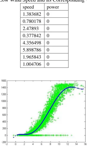
By analyzing the wind speed and wind power which will be used to do the carving fitting, we found that when wind speed was very low and changed suddenly to a high speed, and then quickly went back to low speed, the wind power of the high speed point was 0W likes that of very low wind speed, such as

Table II-1. These points affected the accuracy of the carving fitting Figure II-1, so we eliminate these points before the carving fitting.

Table II-1 Low Wind Speed and Its Corresponding Wind Power speed power 1.383682 0 0.780178 0 2.47893 0 0.377842 0 4.356498 0 5.898786 0 1.965843 0 1.004706 0

Figure II-1 5th-order Carving Fitting without Eliminating the Zero Points

C. Order of Carving Fitting

In the progress of the carving fitting of wind speed and wind power, the order of carving fitting should be taken into consideration as it greatly affects the results of convergence. To decide the order of the carving fitting, this paper makes contrast of 7 different orders to find out the most suitable one for its convenience and accuracy. In Figure II-3 the green spot stands for the actual value and the blue one is the fitted data.

Figure 1(a) Figure 1(b)

Figure 1(c) Figure 1(d)

Figure 1(e) Figure 1(f) Figure II-2. Carving Fitting

(a) 1st-order fitting. (b). 2nd-order fitting. (c) 3rd-order fitting. (d). 4th-order fitting. (e). 5th-order fitting. (f). 7th-order fitting. (g). 10th-order fitting

Figure 2(g)

Figure II-3. Carving Fitting

(a) 1st-order fitting. (b). 2nd-order fitting. (c) 3rd-order fitting. (d). 4th-order fitting. (e). 5th-order fitting. (f). 7th-order fitting. (g). 10th-order fitting

In this paper, we select 7 sets of wind speed and wind power data from different wind turbines and different months randomly. And the results are almost unanimous. Thus these figures are the carving fitting results of one of wind turbines in the same month. From Figure II-3, we can tell that the fifth-order fitting and the seventh-order fitting are very good. And considering the absolute value of the error and the simplicity of carving fitting, we choose the fifth-order fitting as the order of carving fitting in this paper.

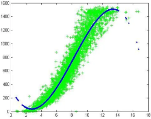
D. Select the Wind Turbine

The data used in this paper starts from March 2011 to January 2012. Use fifth-order for carving fitting to find out one wind turbine with the most optimal data. Firstly carve fitting the wind speed and wind power of 31 wind turbines in March 2011. And calculate the RMS (Root Mean Square) of the actual value and fitted value for each

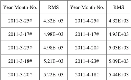
turbine. Then make a list for the wind turbines as the ascending order of RMS, and select the first five wind turbines to carve fitting their data in April 2011. And by comparing the RMS of the five wind turbines in the Table II-2, we choose No.17 as the objective wind turbine. Figure II-4 is the crave fitting of No.17 in March 2011, and the green spot stands for the actual value and the blue one is the fitted data.

Table II-2 RMS of Error of Wind Turbine

Year-Month-No. RMS Year-Month-No. RMS 2011-3-25# 4.32E+03 2011-4-25# 4.32E+03 2011-3-17# 4.98E+03 2011-4-17# 4.93E+03 2011-3-23# 4.98E+03 2011-4-20# 5.03E+03 2011-3-18# 5.21E+03 2011-4-23# 5.09E+03 2011-3-20# 5.22E+03 2011-4-18# 5.44E+03

2.2.

Influencing Factors of Wind Power

In order to analyze the influencing factors of wind power, we start from analyzing the wind turbine capture capacity of wind power. The equation of the wind turbine capture capacity shows below:

3

/ 2

P

PC A v

where, P stands for actual available power(W), C_P refers to the wind power coefficient, Ais the perpendicular area that wind passing through (m2),



Form the equation, wind power varies with the cube of its speed, so wind speed is the most important influencing factor of the wind turbine output. Therefore, wind speed is one of the input variables of neural network.

The wind power coefficient is one of the important parameters stand for the wind turbine efficiency. Every wind turbine has its fixed wind power coefficient, and it indicates the proportion of useful energy obtained by the wind turbine from the wind. According to Bates theory, the maximum of wind power coefficient is 0.593, and the wind power coefficient varies from the type of wind turbines.

For the area that wind passing through perpendicular to the wind,

2 _{/ 4} AD

where Dis the diameter of rotor.

Thus, the air density is the rest of the factors which influence the wind turbine power output, and it is changing over time.

2.2.1 Air Density

Air density is determined by the pressure, temperature and humidity of the air. The equation of the air density shows below:

3.48P(1 0.378 Pb)

T P



 

where P stands for standard atmospheric pressure (kP_a), T is thermodynamic temperature (K), P_b refers to the saturated vapor pressure (kP_a) and



At present, there are different views on whether use the pressure, temperature and humidity as the neural network input in the wind power forecasting research which is based on the meteorological forecast data. The reference [17,18] point out that the correlation of these three variables (pressure, temperature and humidity) and wind power is relatively small. Using them as the neural network inputs has little contribution to improve the effect of the forecasting model, and adding the three variables as the inputs into the neural network will slow down the training speed. Therefore, we do not use the three variables as the inputs in this paper.

2.2.2 Wind Direction

Apart from the influence factor talked about before, wind direction is another important wind power influence factor. As the distribution of wind turbines is scattered, wake flow will be forming after wind passing through the fan blades, and the wind speed will slow down. When the wind speed is low, the wind farm efficiency will reduce in some wind direction as the influence of the wake and roughness. With

the increase of wind speed, the effect of wake flow on the output power will be reduced, and the efficiency coefficient of wind farm will increase. When the wind speed exceeds a certain value, the wind farm efficiency coefficient is 100% in any wind direction. Normally, because the wind changes randomly, the wind farm efficiency coefficient cannot stay 100% all the time. However, because of the relationship between wind power and wind direction is difficult to carve fitting, it is hard to determine the quality of the wind direction. In this paper, the wind direction is not considered as one of the inputs of the neural network. And in this way, the training speed can be faster and the difficulty of network training caused by the wind direction normalization can be prevented. In the further study, the wind direction can be taken as the inputs for more accurate prediction.

2.2.3 Wind Speed

Wind speed has different varying patterns in different length of time, different height and different area. And the change of wind speed is also related to temperature. Meanwhile, the distribution of wind speed is not the same as well. General Weibull distribution is used to describe the statistical distribution of wind speed.

The time scale has an important significance for the study of wind power, and wind power researches under different time scales have different effects on the power system decision-making. Long term wind power forecasting involves in national policies, regulations and energy resources long-term planning, so its uncertainty is quite strong. Use grey modeling to deal with the impact of its uncertainty and predict

the installed capacity and the output of the wind power system [19]. Most wind power forecasting researches are focused on the medium and short term forecasting [20]. The accurate and effective wind power forecasting of wind farm is not only the important reference which helps the power system dispatching operation personnel make the most effective decisions, but also for the reference for the amount of wind power integration under the condition of electricity market. In this paper, we focus on the wind speed and wind power forecasting under time scales of 10min, 1h and 3h.

A. Data Processing

The data we use in this paper is selected from SCADA (Supervisory Control and Data Acquisition) system. And time sampling interval of the data is 10min. Generally, the variation of wind speed doesn’t exceed 6m/s within an hour. And by exploring the data, we find that some wind speed is negative when the wind speed is quite slow. However, it is not correct that the wind speed is negative. Therefore, we should deal with the raw data before considering the sampling frequency is not high.

Firstly, we deal with the negative wind speed. By analyzing the data trending, the negative wind speed is assigned the value zero.

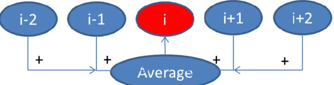
Then, we find out the wind speed which does not meet the condition that the variation of wind speed doesn’t exceed 6m/s within an hour, and calculate the average value of the successively four wind speed. And the bad data v_i is replaced by the average value of v_i-2, v_i-1, v_i+1 and v_i+2.

Figure II-5. Bad Data Replacement

B. Training Matrix

The matrix for neural network training is composed of the wind speed in the chronological order. The number of columns of the training matrix is the number of training data set, and the number of rows of the training matrix is the number of training data in each training set.

For the training matrix, there is a relationship between the adjacent columns. The first data of a column is the second data of previous column, and the rest data arranges in the chronological order in each column.

For example, data a_i,2 is the second data of column i, then, according to the rule of the matrix generating, a_i1,1the first data of column i+1 is equal toa_i,2. So a_i1,2the second data of column i+1 is equal toa_i,3 which is the third data of column i.

Table II-3 Example of Training Matrix

In this way, we get the training matrix. The numbers of columns and rows vary from

column i column i+1 column i+2

… … … ... … … ,2 i

a

a

a

a

=

a

a

=

a

a

a

=

a

a

a

different time scales, and we will discuss later.

C. Testing Matrix

For the testing matrix, the number of rows of testing matrix is the same as the training matrix. However, the number of columns of testing matrix is up to the test data and there is no relationship between any two columns. And the rest data arranges in the chronological order in each column.

III.

WIND SPEED FORECASTING

3.1.

Introduction

Due to Neural Network can approximate any nonlinear mapping through its learning ability, it can be applied to the forecasting of nonlinear system in the time series prediction [21].

First, this section introduces the basic concept and principle of Neural Network. Then, we build the BP neural network forecasting model and AdaBoost_BP improved forecasting mode on Matlab software. And make the short-term wind speed forecasting based on the actual historical data collected from wind farms. Finally, analyze the results of each forecasting model and make contrast.

3.2.

The Basic Principle of Artificial Neural Network

Neural Network (NN), also called as Artificial Neural Network (ANN) or Neural Computing (NC), is to abstract and model the human brain or biological neural network. It has the ability that can learn from the circumstance and adapt to the environment by the interaction similar to that between organisms to achieve the information handle ability which is similar to brain, like learning, recognition, memory, etc [22].

Neural Network not only has the good non-linear ability and the adaptive ability, and it also has the associative learning ability and strong fault tolerance. Therefore, in the

aspect of forecasting there is a large development space and good practical application for Neural Network.

Specifically, Neural Network has the following advantages: [23]

1) Because the information is scattered stored in the neuron of Neural Network, Neural Network has strong robustness and fault tolerance.

2) By using parallel processing method, the structure of Neural Network is parallel and each unit of Neural Network can run the similar progress at the same time. And improve the computation speed in this way.

3) Neural Network can deal with the uncertain or unknown system for its self-learning, self-organizing, adaptivity, various connections between neurons and certain plasticity of the structural junctions between neurons. Neural Network can be trained by using the actual statistics data, and the trained network has the extensive adaptability, which means Neural Network can work even the inputs are not provided in the training. And Neural Network can be trained online.

4) Neural Network can approximate any complex non-linear relationship. For the modeling and forecasting of complex nonlinear systems, neural network is more practical and economical than other methods.

5) Neural network has strong information comprehensive ability. It can handle quantitative and qualitative information at the same time, coordinate the relationship of a variety of input information and deal with complex non-linear and uncertain objects.

nonlinear process which involves various factors. The No.4 and No.5 advantages of Neural Network are a suitable for this part. In addition, the wind power farm is flexible, in other words it is general stage construction. The No. 3 advantage of Neural Network can works with the changing object of forecasting. And No.2 advantage of Neural Network marches the high computation speed requirement of the online wind power forecasting. Therefore, it will largely simplify the modeling work and improve the forecasting precision by selecting Neural Network method for the nonlinear forecasting research on the wind speed and power.

3.2.1 Neuron Model

Neuron is the basic data processing unit of Neural Network, and it is also a nonlinear component with multiple inputs and single output. The inputs of neurons are the external inputs or the outputs of other neurons in the Neural Network, and they determine the response of the neuron. There are three important parts of the neuron: A. Connection Weight

Input x_i connects to Neuron k through Path

i

B. Sum Function

Add the inputs of one neuron (the external inputs or the outputs of other neurons in the Neural Network) together to get the sum of the weighted value.

C. Transfer Function

output of the neuron. The transfer function can limit the amplitude the neuron output. Generally, the range of the amplitude is [0,1] or [-1,1].

Transfer function, also called as excitation function, describes the transfer characteristic of the neurons. Its basic function is:

a) controlling the activation of inputs to output, b) the function transformation of inputs and output,

c) transforming the inputs which may be the infinite range to the limited range output.

The relationship of the inputs and output can be described in the formula below [24]:

1 n i i i I w x   



where, x_i stands for the inputs (the external inputs or the outputs of other neurons),

 refers to the threshold value, w_{i is the connection weight stands for the strength}

of the connection , and f x( ) _{is the excitation function or transfer function.}

For simplicity, take  as the weight of x_{0 which identically equal to 1. And the}

formula will be:

0 n i i i I w x  



3.2.2 Commonly Used Transfer Function

transfer function determines the different characteristics of the neuron output.

Figure III-1. Commonly Used Transfer Functions

A. Threshold Function

In Figure III-1, (a) and (b) are the threshold functions. This function turns any input to two kinds of output ±1 or (0,1).

When y_i equal to 0 or 1, f(x) is the step function shows in (a). ( ) f x 









When y_i equal to -1 or 1, f(x) is the sign function (sgn) shows in (b).

 









Its main feature is non-differentiable and step type. And it often uses in Perceptron Model, M-P Model and Hopfield Model.

B. Saturated Function

In Figure III-1, (c) is the saturated function. Its formula shows:

( ) f x  1 1 1 1 1 1 x k kx x k k x k   _     _{ }   _{ }     _ _   _{ }     _{ }   

Saturated function is essentially the combination of the threshold function and the linear function. Its main feature is non-differentiable and step type. And it often uses in Cellular Neural Network, such as Pattern Recognition, Character Recognition or Noise Control, etc.

C. Hyperbolic Function

In Figure III-1, (d) is the hyperbolic function, also called as sigmoid symmetric function. Its formula shows:

 

Its main feature is differentiable and step type. And it often uses in BP Model or Fukushina Neocognition Model.

D. Sigmoid Function

In Figure III-1, (e) is the sigmoid function. Its formula shows:

1 ( ) 1 I f x e  

The relationship between the input and the neuron state is a monotone function which can value continuously in (0, 1). When   , sigmoid function trends to step function. Generally,  equals 1. Similar to the hyperbolic function, it often uses in

BP Model or Fukushina Neocognition Model.

E. Gaussian Function

In Figure III-1, (f) is the Gaussian function:





where, c _{stands for the central value of Gaussian function, and the function is}

longitudinal axisymmetric when c equals to 0 threshold value.

b

of Gaussian function， and it determines the width of the Gaussian function.

Hyperbolic Function, Sigmoid Function and Gaussian function are continuous transfer function.

3.2.3 Neural Network Structure

The structure of Neural Network largely determines the effect of neural network, and the learning algorithm of Neural Network is selected according to the structure of Neural Network. Therefore, choosing a suitable Neural Network structure, according to the specific problem, for the system identification, modeling or forecasting is an important step in establishing the neural network model. Neural Network can be classified in forward and feedback neural network according to the network structure. They are also known as can be static neural network and dynamic neural network. In this paper, there are the brief introductions of single layer forward neural network, multilayer forward neural network and Elman neural network.

Single layer forward neural network connects the input variables and output directly by one layer of neurons. It complete the training of network by adjusting the deviation b and weightw_ij

B. Multilayer forward neural network

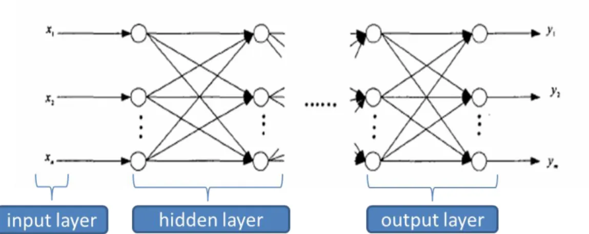
The neurons of Multilayer forward neural network connect with the neurons of one or two adjacent layer. The first layer is input layer, the middle is the hidden layer and the last layer is output layer. Neural Network has one or multiple hidden layers. In the network, adjacent layers connect each other in interconnect mode. There is no link between the neurons in the same layer and there is no feedback loop in the whole network. And there is no direct connection between the input layer and output layer. Hidden layer is used as the intermediary of the external inputs and the network output.

C. Elman Neural Network

Elman feedback Neural Network is a kind of two layers neural network with feedback. Feedback connects to the inputs from the output of first layer by delaying and storing. The number of feedback neurons is the same as that of the neurons of hidden layer, and its input is one step delay of the output of hidden layer neurons.

3.2.4 Neural Network Training

After determined the construction of Neural Network model, Neural Network needs to establish the model to solving a specific problem by learning and training. The

training process of Neural Network is a adjusting the weights of network. The weight of network is the only element for the performance of Neural Network processing unit. Therefore, adjusting the connection weights can make processing unit reflect the model of the given data correctly.

The Neural Network learning aims to reduce the error caused by equations by adjusting the network parameters, such as weights and thresholds of the network which can storage the knowledge from learning stage, according to previous experience. Generally, learning algorithms can be divided into supervised learning method and unsupervised learning method.

In supervised learning method, inputs and the actual output sometimes are requested. Based on the current output and the required target output, the network will adjust the network parameters until the network complete the study of the desired response. A supervised learning process is a closed loop adjustment process from the output to the inputs. On the contrary, the learning progress of the unsupervised learning method just needs a certain number of input learning samples, and the network can make the response to the input patterns without the output learning samples.

In this paper, all the trainings of the neural network forecasting model use the supervised learning algorithm.

3.3.

BP Neural Network

from the adjustment of the network weight is backward propagation learning algorithm. BP learning algorithm was put forward by Rumelhart in 1986. Since then, the BP Neural Network was obtained in a wide range of practical applications. According to statistics, 80% - 90% of Neural Network models adopt BP network or its transformation form.

Figure III-2. BP Neural Network

Figure III-2 [26] is the BP Neural Network diagram. The signal propagation of the network consists of two parts, the forward and backward propagation. In the forward propagation stage, learning samples feed into the input layer, and send to output layer after the step by step operation of hidden layer. The neuron state of each layer only affects the neuron state of next layer. If the output layer did not get the desired output, that is there is an error between the network actual output and the desired output, calculate the error of the output layer, and then go to the error back propagation stage. At this time, the error signal goes back to the input layer from the output layer along the original connection. Then adjust the connection weight layer by layer to make the error minimize.

BP neural network has been used in a variety of forecasting process, and achieved good effects. Therefore, the classical BP Neural Network is one of the choices in this paper.

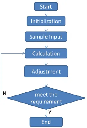
3.3.1 Steps of BP Neural Network Learning Algorithm

（1） Initialization: In this progress, all weighting coefficient are set to be the smallest random number.

（2） The input vectors x₁, x₂,… , x_n and the desired output vectors t₁, t₂,… ,

n

t are the training sets for the network.

（3） Calculate the actual output of each neuron of the hidden layer and output layer.

（4） Get the error of the desired output and the actual output based on Step 3.

（5） Adjust the weighting coefficients of output layer and hidden layer based on Step 4.

（6） If the error did not meet the requirements, continue the progress by returning to Step 3.[27]

Figure III-3. BP Neural Network Learning Steps

3.3.2 The Short-term Wind Speed Forecasting Based on BP Neural Network Learning Algorithm

In this paper, by wind turbine selection we decide to use the data of No.17 wind turbine in 2011 as the sample data. And the forecasting time scales are 10min, 1h and 3h.

A. Matlab Used in Wind Speed Forecasting Based on BP Neural Network

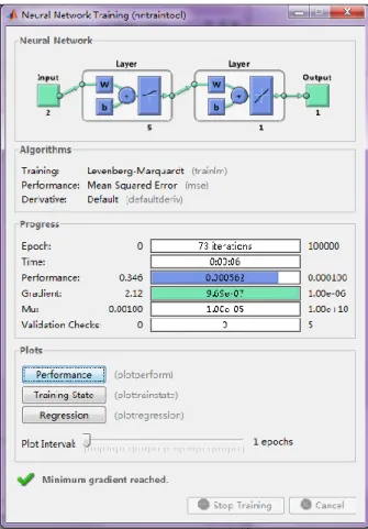
In Matlab software, there is a Matlab neural network toolbox which based on artificial neural network theory [28]. The BP Neural Network in this sample can be established by calling three functions newff , sim and train, in Matlab neural network toolbox. Figure III-4 is the BP Neural Network model built in Matlab software.

Figure III-4. BP Neural Network Model in Matlab

The function of newff _{is mainly setting parameters of the BP neural network. The}

functional form shows in two ways.

a) netnewff P T( , ,









Where:

P: R x Q1 matrix of Q1 sample R-element input vectors T: SN x Q2 matrix of Q2 sample SN-element target vectors

Si: Size of i_th layer, for N-1 layers, (Default = [Output layer size SN is determined from T].)

TFi: Transfer function of i_th layer. (Default = 'tansig' for hidden layers and 'purelin' for output layer.)

BTF: Back propagation network training function (Default = 'trainlm') BLF: Back propagation weight/bias learning function (Default = 'learngdm') IPF: Row cell array of input processing functions.

(Default={'fixunknowns','removeconstantrows','mapminmax'}) OPF: Row cell array of output processing functions.

(Default={'removeconstantrows','mapminmax'}) DDF: Data divison function (Default = 'dividerand')

Usually, the first six parameters are mainly set. P is the input data matrix, and in this sample, P is the matrix form of the wind speed history data arranged for network training. T is the output data matrix which is used to store the result of the short-term wind speed forecasting, and its function is similar with input data matrix.

b) netne ffw (PR S S, 1 2 ...









TFi： Transfer function of i_th layer, Default = 'tansig'.

BTF： Back propagation network training function, Default = 'trainlm'. BLF： Back propagation weight/bias learning function, Default = 'learngdm'. PF： Performance function, Default = 'mse'.

The first expression has less training times than the second one, but the training accuracy of the first one is less than that of the second one. In this study, we take the second expression.

The number of input layer node is the number of wind speed which is prior to the forecasting moment in each time scales. In this paper, we will discuss three time scales. We will discuss the most suitable number of the training data for each training sets for each time scale, so the input layer node numbers of each time scales are not the same. In this sample, the hidden layer node number is set to be 5. Output layer node number is 1, that is, the predicted value export through the Neural Network.

In this sample, we adopt the linear transfer function (purelin function) from the node transfer functions and the BP gradient descent training algorithm function (trainglm) from BTF training function. The last parameters which needs to set is network learning function BLF, and we choose learngdm which has the momentum as the network learning function.

For the whole network, we also need to set its training function and forecasting function.

The functional form of the BP neural network training function is:





As the newff function has already been set, we can call the input data matrix, output data matrix directly to set the parameters of the training function. The last two parameters are used to initialize the conditions of the input and output layer. Generally, they are set as the system default parameters, and there is no do need to decide by ourselves.

In the training function, we need to set the learning rate, and it is set to be 0.05 in this paper (general range is 0.01-0.8). In order to ensure the stability of the system, generally choose the small learning rate. Besides, we also need to select an appropriate expected objective error, and the expected objective error in this sample is set to be 0.0001. And setting an appropriate iteration number can prevent that neural network go into an iteration for not reaching the expected objective. The iteration number in this sample is 100000.

The last function for the wind speed BP Neural Network forecasting modeling in Matlab neural network toolbox is the forecasting function. The functional form of the forecasting function is:

( , )

ysim etn x

Where netis the BP Neural Network model which is established in the newff

function and well trained by the training function train. The x is the history wind speed input used to forecast. As the network is already trained, the functional relationship between the input and the forecasted value can be established by the functions, and get the objective forecasted wind speed at last.

B. Wind Speed Forecasting by BP Neural Network

According to the mathematical analysis above and the optimization algorithm referred, we can make short-term wind speed forecasting with the sampling points we get from SCADA system. The number of the input and output layer in the forecasting process can be set according to the number of independent variables and dependent variables

of the function.

In this paper, we will talk about the wind speed forecasting in the time scales of 10min, 1h and 3h in the future. As the sampling interval is 10min, the data used for 10min forecasting is the sampling data and there are two ways of building the training data for 1h and 3h forecasting that we select. For example, we can use the average hourly value as the element of the input matrix of the training function in 1h forecasting, so the time scale of the element of input matrix is the same as that of the forecasting. We name this model as the single-step wind speed forecasting model. And the second way for 1h forecasting is different in two places. One place is the element of the input matrix of the training function which is the sampling value of 10min in the second way, and the other place is the result of the forecasting which is the average hourly value of six 10min forecasting speeds in the hour. For the forecasting characteristic of the six speeds which we will talk about later, we call this model the iterative multi-step wind speed forecasting method.

a) The single-step and iterative multi-step wind speed forecasting model

The wind speed forecasting models are for the wind speed of 10min, 1h and 3h in the future. As the sampling interval is 10min, the 10min time scale forecasting has only single-step wind speed forecasting model, while 1h and 3h time scale have both single-step and iterative multi-step wind speed forecasting model. i. The single-step wind speed forecasting model

For 10min time scale forecasting model, the element of the neural network training input matrix is the wind speed of every 10min sampling interval, and

the element of training output matrix is the wind speed of 10min in the future. The testing result is the wind speed of 10min in the future.

For 1h time scale forecasting model, the element of the neural network training input matrix is the hourly wind speed which is the average of six adjacent 10min sampling intervals, and the element of training output matrix is the wind speed of 1h in the future. And the testing result is the wind speed of 1h in the future.

For 3h time scale forecasting model, the element of the neural network training input matrix is the wind speed which is the average of eighteen adjacent 10min sampling interval, and the element of training output matrix is the wind speed of 3h in the future. And the testing result is the wind speed of 3h in the future.

ii. The iterative multi-step wind speed forecasting model

For 1h time scale forecasting model, the element of the neural network training input matrix is the wind speed of every 10min sampling interval, and the element of training output matrix is the wind speed of 10min in the future. The element of the testing result is the hourly wind speed which is the average of six adjacent 10min forecasting wind speeds. The first 10min forecasting wind speed is Y₁, and the testing input matrix of Y₁ is composed by z _{10min sampling intervals. The second forecasting wind speed is} Y₂, and the testing input matrix of Y₂ is composed by z1 _{10min sampling}

composed by z2 _{10min sampling intervals and} Y Y₁, _{2 as the last two} elements of the matrix. Y₄ is composed by z3 _{10min sampling intervals}

and Y Y Y₁, ,_{2 3 as the last three elements of the matrix.} Y₅ is composed by

4

z _{10min sampling intervals and} Y Y Y Y₁, ₂, ,_{3 4 as the last four elements of} the matrix. Y6 is composed by z5 10min sampling intervals and

1, 2, ,3 4, 5

Y Y Y Y Y _{as the last five elements of the matrix. And the testing result is}

the average value of Y Y Y Y Y Y₁, , , , ,_{2 3 4 5 6 which stands wind for speed of 1h in} the future.

Table III-1 Element of Multi-step Wind Speed Forecasting Matrix

For 3h time scale forecasting model, the element of the neural network training input matrix is the hourly wind speed which is the average of six adjacent 10min sampling intervals, and the element of training output matrix is the wind speed of 1h in the future. The element of the testing result is the wind speed of 3h in the future which is the average of 3 adjacent 1h

column i column i+1 column i+2 column i+3 column i+4 column i+5

… … … … … … … … … … … … … … … … … 10min Forecasting Speed Training Input Matrix 1h Forecasting Speed = ,2 i

a

a

a

a

=

a

a

=

a

a

=

a

a

a

a

a

forecasting wind speeds. The first 1h forecasting wind speed is Y₁, and the testing input matrix of Y₁ is composed by z hourly wind speeds which is the average of six adjacent 10min sampling intervals. The second forecasting wind speed is Y₂, and the testing input matrix of Y₂ is composed by z1

hourly wind speeds and Y_{1 as the last one element of the matrix.} Y₃ is composed by z2 _{hourly wind speeds and} Y Y₁, _{2 as the last two elements} of the matrix. And the testing result is the average value of Y Y Y₁, ,_{2 3 which} stands wind for speed of 3h in the future.

Here is Table III-2 of the single-step and iterative multi-step wind speed forecasting model.

Table III-2. Single-step and Iterative Multi-step Wind Speed Forecasting Model

b) The number of the training data for each training sets

When we established the BP Neural Network of wind speed forecasting model, we found that the number of the training data for each training matrix, that is to say the length of the column of the training matrix, affected the final result of the accuracy of forecasting speed.

Therefore, we want to find the optimal number of the training data for each

training input wind speed training output wind speed testing result wind speed 10min sampling interval 10min in the future 10min in the future

single-step average of 1h sampling wind speed 1h in the future 1h in the future multi-step 10min sampling interval 10min in the future 1h in the future single-step average of 3h sampling wind speed 3h in the future 3h in the future multi-step average of 1h sampling wind speed 1h in the future 3h in the future Model 10min 1h 3h 1, 2, 3, 4, 5, 6 6 Y Y Y Y Y Y 1, 2, 3 3 Y Y Y