ASU: An Experimental Study on Applying Deep Learning in Twitter Named Entity Recognition

(1)

ASU: An Experimental Study on Applying Deep Learning in Twitter

Named Entity Recognition

Michel Naim Gerguis, Cherif Salama, M. Watheq El-Kharashi

Computer & Systems Engineering Department, Ain Shams University, Cairo, 11517, Egypt

Abstract

This paper describes the ASU system submitted in the COLING W-NUT 2016 Twitter Named Entity Recognition (NER) task. We present an experimental study on applying deep learning to extracting named entities (NEs) from tweets. We built two Long Short-Term Memory (LSTM) models for the task. The first model was built to extract named entities without types while the second model was built to extract and then classify them into 10 fine-grained entity classes. In this effort, we show detailed experimentation results on the effectiveness of word embeddings, brown clusters, part-of-speech (POS) tags, shape features, gazetteers, and local context for the tweet input vector representation to the LSTM model. Also, we present a set of experiments, to better design the network parameters for the Twitter NER task. Our system was ranked the fifth out of ten participants with a final f1-score for the typed classes of 39% and 55% for the non typed ones.

1 Introduction

The social media dominance, especially Twitter, rapidly drives the text processing technologies for more automated understanding. Daily, there are billions of short, noisy, user-generated text fragments that represent and summarize the whole world. Although Natural Language Processing (NLP), in general, is a very challenging task, the importance of automatically processing those huge amounts of big data pushes the technology in dealing with more short and noisy data. The open world of social media, like Twitter, makes it easy for NLP researchers to grasp lots of information to present a holistic view of the world as represented by millions of users. Through NLP research on social media, one can analyze the political polarity of the crowds, identify trending events that attract parts of the world, key people, and hot areas instantaneously, detect emotion storylines and what can lead to or change people’s attitudes, identify and collect data in disasters including natural ones to help in risk management, grasp the sentiment against new products or decisions, understand and predict actions based on opinion mining, and many more. Entity extraction is the basic unit in all these NLP tasks whether to be a singer, president, player, movie, song, or any entity of interest. The coarse-grained classes like person, location, and organization are not sufficient for a better representation and understanding of the vibrant world. That is why the fine-grained NERs are of utmost interest.

Our submission in COLING W-NUT 2016 Named Entity Recognition shared task in Twitter, in its second edition, (Strauss et al., 2016; Baldwin et al., 2015) relied on an experimental study on applying deep learning to the task. We experimented with many representations to define the network’s input vector. The contribution of word embeddings (WEs), brown clusters (BCs), POS tags, a long list of shape features, vocabulary, and gazetteers was experimentally evaluated in details for the NER task. In addition, a series of experiments were directed to best tune our network design. Two different LSTM models were prepared: One for detecting entities regardless of entity type (non typed) and the other was trained for detecting and classifying the entities (typed).

This work is licenced under a Creative Commons Attribution 4.0 International License. License details: http:// creativecommons.org/licenses/by/4.0/

(2)

The rest of the paper is organized as follows; In Section 2, we present the data sets available for the task and how we used them in ASU system. Section 3, illustrates an overview of our system and the process we followed. In Section 4, we present in details our experimental study in an incremental approach in which we experimented with lots of representations one-by-one and also, with the network parameters. Finally, we conclude in Section 5.

2 Data Sets

In this section, we discuss the distribution and the size of the four released data sets for the Twitter NER task. Also, we brief how those data sets were utilized in training our two models and then in submitting the final results.

Data Set Training

Set Dev.Set AdditionalSet TestSet

Num. Tweets 2394 1000 419 3850 Num. Tokens 46469 16261 6789 61908 Num. Entity Tokens 2462 1128 439 5955 Company Tokens 207 49 64 886 Facility Tokens 209 77 13 619 Geo-Loc Tokens 325 158 62 1101

Movie Tokens 80 30 5 82

MusicArtist Tokens 116 76 22 331 Other Tokens 545 229 91 1140 Person Tokens 664 266 113 782 Product Tokens 177 158 15 746 SportsTeam Tokens 74 83 46 195

TvShow Tokens 65 2 8 73

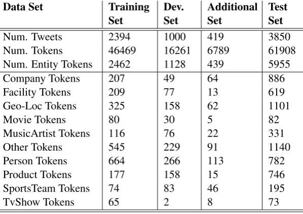
Table 1: W-NUT 2016 Twitter NER Data Sets Statistics. Four data sets were released

for the task. Table 1 indi-cates the four sets along with the total number of tweets per set, the total number of tokens, the total number of entity to-kens, and the total number of entity tokens per entity class for the 10 classes. It is important to note that some of the en-tity classes are not well repre-sented in the data sets like the TvShow, the Movie, and the SportsTeam classes. While the provided data set might repre-sent the real world distribution of the entity classes, we believe that for some classes the data is not enough for deep learning.

ASU system relied on the

training set plus the additional set for training purpose in the whole experimentation study while testing on the development set as discussed in Section 4. After the system was tuned, we re-trained the models using the whole available data, training, development, and the additional sets. These trained models were applied on the test set to submit our final results.

3 Method

In this section, we brief the main methodology we followed to build our two models.

We relied on Microsoft’s computational network toolkit (CNTK)1_{in building up our two models. We}

preferred to tackle the task using an LSTM network to benefit from sequence modeling. The network consists of an input layer, some hidden layers, and an output one. The input layer mainly represents the input tweet in a vector of nodes. The hidden layers of our network consist of an embedding layer and some LSTM layers. We initially set the embedding layer to be a 100-nodes layer and an only one hidden LSTM layer of 200-nodes. For the non typed model, the output layer of the network consists of only two nodes, one to detect entities and the other for non entities, while the typed model’s output layer is represented by eleven nodes, one for each entity class and the last one for non entities.

For the experimentation procedures we conducted, first we pass the training data through an encoding component in order to convert the raw tweet into a vector which is the input representation of the network. Based on the experiment’s feature representation, we produce a mapping function that maps the features into some identifiers. Using the same mapping function, we encode the development set. Then, we design the CNTK configuration file for the network by adjusting the input vector size, the output one,

[image:2.595.231.530.223.434.2]

(3)

and the whole network parameters. We then, train the two models and test over both the training set and the development one. Finally, we score our results and decide whether to include this feature in the main flow or discard it. We adopted an incremental approach in which we fix all the parameters and change only one to assess the value of adding/removing it.

4 Experiments and Results

[image:3.595.78.520.296.474.2]

In this section, all experiments we conducted are presented with details in how we built our LSTM models: Basically, we have two models. One for the non typed extractions and the other for the typed ones which work on ten entity classes. Figure 1 illustrates our experimentation efforts for the typed model while Figure 2 summarizes the history of the non typed model. We plot the f1-scores of the overall system on the training and the development sets for both models. Each experiment in the figures is given an integer identifier which will also be used in the following subsections. While we report the progress in the coming subsections, we preserved the best system as the first record in each table for reference. Also, we appended the index for the previous experiment on which we based the new experiment.

Figure 1: ASU incremental approach f1-scores for Typed LSTM model on Training/Dev. Set.

[image:3.595.81.521.543.724.2]

(4)

4.1 ASU Incremental Approach

In the coming subsections, we present the input vector evolution for our network and also our experiments in the network design. This study shows how our experimentation incrementally moved the overall f1-score in the typed model from 0% to about 43% in the last one on the development set (Figure 1).

4.1.1 POS Tags

Our experimentation started by deciding which POS tagger to use. We experimented with OpenNLP model (Morton et al., 2005), TweetNLP model (Owoputi et al., 2013; Gimpel et al., 2011), and Ritter’s model (Ritter et al., 2011). While TweetNLP relied on a tagset of 25 tags, the two other taggers followed Penn Treebank tagset. We represented each token by its POS tag, just the current token. Table 2 reports the f1-scores for each tagger on the training and development sets for the typed model and the non typed one. We decided to use TweetNLP as it showed the best results. We then, experimented with the POS tags for some more context. In experiment 4, we added the POS tags for a window of only one token, the token before and the token after, while in experiment 5, we extended the representation for each token to a context window of two. Minor gains were introduced to claim the saturation so we finalized POS tags representation to be a windows of two.

ID Experiment Description Train. Set:

Typed Dev. Set:Typed Train. Set:Non Typed Dev. Set:Non Typed

[image:4.595.90.509.291.388.2]

1 POS Tags: OpenNLP 00.00% 00.00% 13.85% 12.80% 2 POS Tags: Ritter 00.0% 00.00% 27.05% 25.42% 3 POS Tags: TweetNLP 00.00% 00.00% 40.67% 33.12% 4 3 + POS Tags: Context (1) 15.11% 12.37% 44.69% 36.39% 5 4 + POS Tags: Context (2) 16.44% 12.42% 46.10% 37.27%

Table 2: POS Tags in ASU for Typed/Non Typed Models on the Training/Dev. Sets.

4.1.2 Brown Clusters

We experimented with the tweets brown clusters2_{(Owoputi et al., 2012) in various binary prefix lengths.}

We believe that BCs out of twitter data could be of more relevance (Derczynski et al., 2015; Cherry et al., 2015) than other sources like Wikipedia (Yang and Kim, 2015). Table 3 summarizes the f1-scores for each prefix length incrementally. Our experimental study indicates that brown clusters’ prefixes of 4, 8, and 10 are the best. Contextual brown clusters for a window of one reported minimal gains.

[image:4.595.86.507.528.709.2]

5 4 + POS Tags: Context (2) 16.44% 12.42% 46.10% 37.27% 6 5 + BCs: Len. 4 24.33% 18.07% 47.19% 38.82% 7 6 + BCs: Len. 8 28.32% 22.15% 48.60% 38.73% 8 7 + BCs: Len. 12 29.55% 23.36% 53.71% 44.36% 9 8 + BCs: Len. 6 32.03% 23.88% 53.72% 44.70% 10 9 + BCs: Len. 10 37.44% 27.84% 57.16% 47.90% 11 10 + BCs: Context (1) Len. 4 40.76% 27.84% 57.56% 48.62% 12 11 + BCs: Context (1) Len. 6 40.41% 30.45% 58.96% 48.34% 13 12 + BCs: Context (1) Len. 8 41.90% 31.15% 60.51% 49.19% 14 13 + BCs: Context (1) Len. 10 45.05% 32.32% 63.09% 49.10% 15 14 + BCs: Context (1) Len. 12 45.67% 30.96% 65.59% 49.54%

Table 3: Brown Clusters in ASU for Typed/Non Typed Models on the Training/Dev. Sets.

(5)

4.1.3 Word Embeddings

ASU system utilizes Google’s word embeddings models Word2Vec3_{which are based on 300 dimensional}

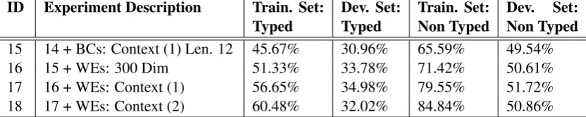
vectors (Mikolov et al., 2013). We believe that generating embeddings out of tweets would boost the results (Toh et al., 2015). In experiment 16, 300 nodes of WEs were added to the input representation. Context window of one and two were also tested in experiments 17 and 18 respectively. Enhancements in the results on the training set were noticed when we added the context window of two, while regressions on the development set which we classified as a sort of over-fitting so we discard it. Table 4 summarizes the three WEs experiments in ASU.

[image:5.595.91.507.186.269.2]

15 14 + BCs: Context (1) Len. 12 45.67% 30.96% 65.59% 49.54% 16 15 + WEs: 300 Dim 51.33% 33.78% 71.42% 50.61% 17 16 + WEs: Context (1) 56.65% 34.98% 79.55% 51.72% 18 17 + WEs: Context (2) 60.48% 32.02% 84.84% 50.86%

Table 4: Word Embeddings in ASU for Typed/Non Typed Models on the Training/Dev. Sets.

4.1.4 Shape Features

So far, the token itself is not represented in the input vector. A list of shape features was collected from previous efforts (Akhtar et al., 2015; Toh et al., 2015) and then extended to reach the following set of 11 features:

1. StartsWithUpper, whether the token starts with an upper letter. 2. StartOfTweet, whether the token is the first one in the tweet. 3. AllUpper, whether the token is all capitalized.

4. TweetAllUpper, whether the tweet is all capitalized.

5. ContainsUpper, whether the token contains a capital letter other than the first one. 6. IsAplhaNumeric, whether the token contains numbers and letters.

7. AllDigit, whether the token is a digit or a decimal number. 8. AllPunc, whether the token is a punctuation or a symbol.

9. ContainsPunc, whether the token contains a punctuation or a symbol letter. 10. IsHashTag, whether the token is a hashtag, starts with a # marker.

11. IsTag, whether the token is a twitter tag, starts with an @ marker.

Table 5 shows results obtained when the shape features were added. We got some enhancements when we applied the shape features to the token itself while when we appended the shape features for the token before and the token after, creating a context window of size one, regressions were noticed.

17 16 + WEs: Context (1) 56.65% 34.98% 79.55% 51.72% 19 17 + Shape 57.40% 37.28% 83.70% 56.89% 20 19 + Shape: Context (1) 56.47% 37.30% 87.24% 56.32%

Table 5: Shape Features in ASU for Typed/Non Typed Models on the Training/Dev. Sets.

(6)

4.1.5 Non Entity Features

We then, started to rely on some dictionaries. Two new nodes were added in the input representation. One to indicate whether the token is a stop word or not and the other to mark being a frequent lower word. We relied on the available dictionaries which lead to a slight regression in the non typed model results. We believe that the top 10K lowered words are not enough so it needs further additions. With simple error analysis, we found lots of tokens not in the lower list like Sunday and club for example. We also, experimented with those two features in a context window of one showing reasonable gain as summarized in Table 6.

19 17 + Shape 57.40% 37.28% 83.70% 56.89% 21 19 + IsStop IsLower 57.58% 37.47% 85.50% 56.39% 22 21 + IsStop IsLower: Context (1) 62.35% 38.61% 84.69% 56.36%

Table 6: Non Entity Features in ASU for Typed/Non Typed Models on the Training/Dev. Sets.

4.1.6 Vocabulary Features

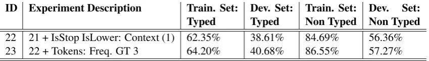
To represent the vocabulary of the tokens, we collected a unique list of the tokens in the training data sorted descendingly by frequency of occurrences. A threshold of 3 was used to select the top 1.75K tokens to be represented in the input vector. As Table 7 shows, a good gain could be noticed due to adding the vocabulary information to the input vector representation.

[image:6.595.88.513.386.447.2]

22 21 + IsStop IsLower: Context (1) 62.35% 38.61% 84.69% 56.36% 23 22 + Tokens: Freq. GT 3 64.20% 40.68% 86.55% 57.27%

Table 7: Vocabulary in ASU for Typed/Non Typed Models on the Training/Dev. Sets.

4.1.7 Embedding Layer Size

Next, we focused on the network design itself. The defaults used in all previous experiments were a 100-nodes embedding layer followed by a single 200-100-nodes hidden layer. We tried out various sizes for our embedding layer to find out that a 150-nodes layer added two more f1-score points to our typed system as shown in Table 8.

23 22 + Tokens: Freq. GT 3 64.20% 40.68% 86.55% 57.27% 24 23 + EM: 50 56.59% 34.61% 80.92% 55.91% 25 23 + EM: 150 68.28% 42.76% 89.12% 57.02% 26 23 + EM: 200 70.95% 40.03% 89.54% 57.00% 27 23 + EM: 300 69.15% 41.97% 90.37% 56.36%

Table 8: Embedding Layer Size Tuning in ASU for Typed/Non Typed Models on the Training/Dev. Sets.

4.1.8 Hidden Layer Size

(7)

score in movie and tvshow classes. Only the scores of those two classes did not improve along with all previous experiments, so we preferred the 400-nodes hidden layer.

ID Experiment

Description Train. Set:Typed Dev. Set:Typed Train. Set:Non Typed Dev. Set:Non Typed

25 23 + EM: 150 68.28% 42.76% 89.12% 57.02% 28 25 + HL: 1 * 150 54.79% 34.20% 88.67% 57.40% 29 25 + HL: 1 * 250 68.16% 41.74% 88.60% 58.39% 30 25 + HL: 1 * 300 68.26% 40.16% 88.49% 56.66% 31 25 + HL: 1 * 400 78.18% 41.91% 88.81% 56.11% 32 25 + HL: 1 * 500 82.47% 41.78% 89.58% 56.18%

Table 9: Hidden Layer Size Tuning in ASU for Typed/Non Typed Models on the Training/Dev. Sets.

4.1.9 Number of Hidden Layers

Another dimension was subject to our experimentation, the number of the hidden layers. The default was just one layer but when we extended to two hidden layers, we experienced a huge loss on the results as Table 10 details. That is why, we stopped investing more time in this direction.

ID Experiment

31 25 + HL: 1 * 400 78.18% 41.91% 88.81% 56.11% 33 31 + HL: 2 * 400 51.00% 32.18% 86.81% 56.67%

Table 10: Number of Hidden Layers Tuning in ASU for Typed/Non Typed Models on the Training/Dev. Sets.

4.1.10 Number of Epochs

The last parameter, we experimented with, in our network design was the number of epochs. The default was to pass by the data 7.5 times in the learning phase. We tried to study the change when our system doubles the times in passing by the whole data. We also, experimented with some more variants as Table 11 summarizes. We favored the SeeData rate of 10 times for the benefit of the typed system.

ID Experiment

31 25 + HL: 1 * 400 78.18% 41.91% 88.81% 56.11% 34 31 + SeeData: 10 83.04% 42.16% 91.56% 55.93% 35 31 + SeeData: 5 71.35% 38.94% 84.64% 56.88% 36 31 + SeeData: 15 89.27% 41.55% 94.75% 54.36%

Table 11: Number of Epochs Tuning in ASU for Typed/Non Typed Models on the Training/Dev. Sets.

4.1.11 Gazetteers

(8)

[image:8.595.83.513.139.223.2]

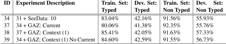
Table 12, showed that the gazetteers negatively affected the system when applied to the current tokens only, experiment 37. When we used them for the token before and after along with the current token, experiment 38, acceptable enhancements showed up. Our last experiment, experiment 39, preserved the gazetteers features for the context windows of one while bypassing the current tokens to show the best results.

34 31 + SeeData: 10 83.04% 42.16% 91.56% 55.93% 37 34 + GAZ: Current 80.06% 41.38% 92.35% 55.76% 38 37 + GAZ: Context (1) 85.41% 42.05% 91.63% 57.33% 39 34 + GAZ: Context (1) No Current 84.60% 42.59% 91.55% 56.73%

Table 12: Gazetteers in ASU for Typed/Non Typed Models on the Training/Dev. Sets..

4.2 Final System

Our final results are reported in details in Table 13. We report our final precision, recall, and f1-score on the training, development, and the testing sets. After we tuned the two models, we appended the training and development sets to act as a new training set for our final model which was used in the final submission as detailed in Section 2.

Type _P Training Set_R _F1 _P Development Set_R _F1 _P Testing Set_R _F1

company 85.44% 86.27% 85.85% 19.75% 41.03% 26.67% 51.18% 31.40% 38.92% facility 82.73% 81.98% 82.35% 32.50% 34.21% 33.33% 21.82% 18.97% 20.30% geo-loc 86.51% 91.61% 88.99% 49.32% 62.07% 54.96% 60.60% 61.56% 61.08% movie 63.16% 64.86% 64.00% 20.00% 20.00% 20.00% 02.78% 02.94% 02.86% musicartist 64.06% 60.29% 62.12% 22.73% 12.20% 15.87% 12.28% 03.66% 05.65% other 66.92% 65.44% 66.17% 32.86% 34.85% 33.82% 21.97% 20.21% 21.05% person 96.56% 96.74% 96.65% 58.51% 64.33% 61.28% 43.45% 64.73% 52.00% product 83.33% 75.47% 79.21% 09.68% 08.11% 08.82% 12.90% 08.13% 09.98% sportsteam 88.24% 87.21% 87.72% 55.81% 34.29% 42.48% 30.41% 40.14% 34.60% tvshow 82.86% 72.50% 77.33% 11.11% 50.00% 18.18% 09.09% 06.06% 07.27% Overall 84.69% 84.50% 84.60% 40.98% 44.33% 42.59% 40.58% 37.58% 39.02% No Types 92.45% 90.67% 91.55% 54.62% 59.00% 56.73% 57.55% 52.98% 55.17%

Table 13: Results of ASU System on Training, Development, and Testing Set.

5 Conclusion

We presented the ASU system in the COLING W-NUT 2016 Twitter NER task. Our system experimen-tally shows an incremental approach in designing two LSTM models: One for entity detection and the other for extracting and classifying a set of 10 fine-grained classes. This study presents experimentally the effect of adding/removing many features in the input representation along with an analysis on the network design. We report a 39% f1-score for the typed model on the test set and a 55% for the non typed one bringing ASU to the fifth place out of ten participants.

(9)

References

Md Shad Akhtar, Utpal Kumar Sikdar, and Asif Ekbal. 2015. Iitp: Multiobjective differential evolution based

twitter named entity recognition. ACL-IJCNLP.

Timothy Baldwin, Young-Bum Kim, Marie Catherine de Marneffe, Alan Ritter, Bo Han, and Wei Xu. 2015.

Shared tasks of the 2015 workshop on noisy user-generated text: Twitter lexical normalization and named entity

recognition. ACL-IJCNLP.

Colin Cherry, Hongyu Guo, and Chengbi Dai. 2015. NRC: Infused Phrase Vectors for Named Entity Recognition

in Twitter.ACL-IJCNLP.

Leon Derczynski, Isabelle Augenstein, and Kalina Bontcheva. 2015.USFD: Twitter NER with Drift Compensation

and Linked Data. ACL-IJCNLP.

Kevin Gimpel, Nathan Schneider, Brendan O’Connor, Dipanjan Das, Daniel Mills, Jacob Eisenstein, Michael Heilman, Dani Yogatama, Jeffrey Flanigan, and Noah A. Smith. 2011. Part-of-speech tagging for twitter: Annotation, features, and experiments. Association for Computational Linguistics.

Thomas Morton, Joern Kottmann, Jason Baldridge, and Gann Bierner. 2005. Opennlp: A java-based nlp toolkit.

https://opennlp.apache.org/.

Tomas Mikolov, Ilya Sutskever, Kai Chen, Greg S. Corrado, and Jeff Dean. 2013. Distributed representations of

words and phrases and their compositionality.Advances in neural information processing systems.

Olutobi Owoputi, Brendan OConnor, Chris Dyer, Kevin Gimpel, and Nathan Schneider. 2012. Part-of-speech

tagging for Twitter: Word clusters and other advances. School of Computer Science.

Olutobi Owoputi, Brendan O’Connor, Chris Dyer, Kevin Gimpel, Nathan Schneider, and Noah A. Smith 2013.

Improved part-of-speech tagging for online conversational text with word clusters. Association for

Computa-tional Linguistics.

Alan Ritter, Sam Clark, and Oren Etzioni. 2011. Named entity recognition in tweets: an experimental study.

Empirical Methods in Natural Language Processing.

Benjamin Strauss, Bethany E. Toma, Alan Ritter, Marie Catherine de Marneffe, and Wei Xu. 2016. Results of the

WNUT16 Named Entity Recognition Shared Task.Workshop on Noisy User-generated Text (WNUT 2016).

Zhiqiang Toh, Bin Chen, and Jian Su. 2015. Improving twitter named entity recognition using word

representa-tions. ACL-IJCNLP.

Eun-Suk Yang and Yu-Seop Kim 2015.Hallym: Named Entity Recognition on Twitter with Induced Word