R E S E A R C H
Open Access
On single-step HSS iterative method with
circulant preconditioner for fractional
diffusion equations
Mu-Zheng Zhu
1*, Guo-Feng Zhang
2and Ya-E Qi
3*Correspondence:
1School of Mathematics and
Statistics, Hexi University, Zhangye, China
Full list of author information is available at the end of the article
Abstract
By exploiting Toeplitz-like structure and non-Hermitian dense property of the discrete coefficient matrix, a new double-layer iterative method called SHSS-PCG method is employed to solve the linear systems originating from the implicit finite difference discretization of fractional diffusion equations (FDEs). The method is a combination of the single-step Hermitian and skew-Hermitian splitting (SHSS) method with the preconditioned conjugate gradient (PCG) method. Further, the new circulant preconditioners are proposed to improve the efficiency of SHSS-PCG method, and the computation cost is further reduced via using the fast Fourier transform (FFT). Theoretical analysis shows that the SHSS-PCG iterative method with circulant preconditioners is convergent. Numerical experiments are given to show that our SHSS-PCG method with circulant preconditioners preforms very well, and the proposed circulant preconditioners are very efficient in accelerating the convergence rate.
MSC: Primary 65F10; 65N22; secondary 26A33; 65T50
Keywords: Fractional diffusion equations; Circulant preconditioner; Toeplitz; Single-step Hermitian and skew-Hermitian splitting; Preconditioned conjugate gradient (PCG) method
1 Introduction
Fractional calculus has a long history and its origin goes back to describing half order (α= 1/2) derivative by Leibnitz in 1695. It was believed that this branch of mathematics had no applications. But in the last thirty years, the fractional derivatives and the frac-tional partial differential equations (FPDEs) have attracted growing attention [1,2], be-cause they can provide an adequate and accurate description of transport processes that exhibit anomalous diffusion behavior in the real word [3,4], including Brownian motion, entropy [5], groundwater contaminant transport [6,7], turbulent flow [8,9], and applica-tions in biology [10], image processing [11], engineering and physics [12–15].
In recent years, a large amount of work has been devoted to finding out how to solve FPDEs [16–18]. The main reason is that it is more challenging or sometimes even impos-sible to obtain the analytical solution of FPDEs, or that the obtained analytical solution is less valuable (expressed by the transcendental functions or infinite series). As a con-sequence, numerical solutions for FPDEs have become the main methods and then have
been developed intensively, e.g., (compact) finite difference methods [19–22], finite ele-ment methods [23,24], discontinuous Galerkin methods [25,26], and other numerical methods [27–29].
However, due to the nonlocality of a fractional differential operator, a naive discretiza-tion of FDEs, even though implicit, leads to uncondidiscretiza-tional instability [30,31]. Moreover, coefficient matrices arising from most numerical discretizations of FDEs are non-sparse and typically require the computational cost ofO(N3) by using Gaussian elimination and
the storage ofO(N2), whereNis the number of grid points [32].
In order to overcome the difficulty of stability, Meerschaet and Tadjeran [30, 31] proposed an unconditionally stable shifted Grünwald discretization to approximate the FDEs, which is based on the equivalence of Grünwald–Letnikov fractional derivative and Riemann–Liouville fractional derivative with some conditions. Later, the Toeplitz-like structure of the full coefficient matrix via Meerschaet–Tadjeran’s method was discov-ered [32,33]; more precisely, such a full matrix can be written as the sum of diagonal-multiply-Toeplitz matrices. Thus, the storage is significantly reduced fromO(N2) toO(N) and the matrix-vector multiplication of Toeplitz matrix can be calculated by using the fast Fourier transform (FFT) withO(NlogN) operations [34–36]. By exploiting such a special structure, Wang and Wang [37] proposed the conjugate gradient normal residual (CGNR) method to solve the discretized system of FDEs with Meerschaet–Tadjeran’s method, and numerically showed that its convergence is fast with smaller diffusion coefficients (in that case the discretized system is well-conditioned). On the other hand, when the diffusion coefficients are not small, the problem becomes ill-conditioned and the convergence of the CGNR method slows down. To avoid the resulting drawback, Lei and Sun [38] pro-posed a robust CGNR method with the circulant preconditioner to solve the FDEs with Meerschaet–Tadjeran’s method under the condition that the diffusion coefficients are con-stant and the ratio xα
t is bounded away from zero. The spectrum of the preconditioned
matrix is proven to cluster around 1 if the diffusion coefficients are constant and the con-vergence rate of the proposed iterative algorithm is superlinear. In 2015, Bai, Huang, and Gu [39] proposed the Hermitian and skew-Hermitian splitting methods and the circu-lant preconditioner to accelerate the convergence rate for solving the fractional diffusion equations with constant coefficients; and numerical results show that the methods and circulant preconditioners are efficient.
The novelty of this paper is to present a new double-layer SHSS-PCG iterative method to further utilize matrix structure to improve the computational efficiency for solving the full non-Hermitian linear systems originating in the discretization of FDEs. The new method includes two aspects. One is that the outer iteration is a single-step HSS (SHSS) iterative method to utilize the fact that the coefficient matrix generated by Meerschaet–Tadjeran’s method is a full non-Hermitian positive definite matrix and its Hermitian part is domi-nant; and the other is that the inner iteration is the classic conjugate gradient (CG) method with circulant preconditioners based on Strang’s and T. Chan’s approximation, to take the full advantage of the Toeplitz structure of the dominant Hermitian part.
dis-cussed. In Sect.5, numerical experiments are given to show the performance of the pro-posed method. Finally, some concluding remarks are given in Sect.6.
2 FDEs and finite difference discretization
In this paper, we consider the following initial-boundary value problem of FDEs:
⎧
to the classical hyperbolic PDEs. The case 1 <α< 2 represents a super-diffusive process, where particles diffuse faster than the classical parabolic PDEs predict [30].
From a numerical point of view, an interesting definition of the right-sided and the left-sided fractional derivatives is the Grünwald–Letnikov form given by
∂αu(x,t)
where·denotes the floor function, andg(kα)is the alternating fractional binomial coeffi-cient given as
where
andI∈RN×Nbe the identity matrix, then the numerical discrete scheme can be rewritten
in a matrix form as follows (see [32]): like matrix, which is asymmetric in general. Furthermore, the storage of Toeplitz-likeA(m) can be reducedO(N) and the matrix-vector multiplication can be obtained in
which is related to the number of time steps and grid points. The linear system (3) can be
In this section, we first introduce the single-step HSS (SHSS) iterative method, and then propose the SHSS-PCG iterative method for solving the discretized linear system (6).
Suppose that the diffusion coefficients are two nonnegative constants, i.e.,d(+,mi)=d+≥0,
d–,(mi)=d–≥0 andd++d–= 0. LetM(m)=H+S, where
Obviously, the above matrix splitting is the Hermitian and skew-Hermitian splitting (HSS).
Based on this splitting, Li [40] proposed using the SHSS iterative method to solve linear system (6).
The SHSS method Given an initial guessx(0), fork= 0, 1, 2, . . . , until{x(k)} converges,
compute
whereβis a given positive constant,HandSare the Hermitian and skew-Hermitian parts ofM(m), respectively.
Obviously, the SHSS iterative method is a single step iterative scheme. The convergence of the SHSS is discussed in [40] and described in the following lemma.
Lemma 3.1([40]) LetM(m)∈Cn×nbe a positive definite matrix,H=1
2(M(m)+M(m)
T
)
and S= 12(M(m)–M(m)T)be its Hermitian and skew-Hermitian parts,respectively.Let
β be a positive constant.Then the spectral radiusρ(T(β))of the iteration matrix T(β) = (βI+H)–1(βI–S)of the SHSS iterative method is bounded byδβ=β2+σmax2
β+λmin ,whereλminis the
smallest eigenvalue of matrix H andσ2
maxis the largest singular value of matrix S.Moreover,
it holdsρ(T(β))≤δβ≤1whenβ>σmax2 –λmin
2λmin ,i.e.,the SHSS iterative method converges to
the unique solution x∗of(6).
Since it is very costly and impractical to obtain the exact solution, the linear problems in (9) are solved iteratively and approximately in practice. ConsideringβI+His Hermitian positive definite and its Toeplitz-like structure is exploited, we may employ the CG method with some circulant preconditioners to solve approximately the linear systems. Thus, we may obtain a new iterative method, called SHSS-PCG method.
More clearly, we rewrite this SHSS-PCG iterative method with circulant preconditioner
Pfor solving the non-Hermitian full linear system (6) as the following scheme (Algorithm1 and Subroutine1).
Next, we introduce two circulant preconditioners for Toeplitz matrixT= (ti–j)0≤i,j≤N.
One is based on Strang’s circulant approximation, called Strang’s preconditioners(T) [41], which is defined to be the circulant matrix obtained by copying the central diagonal ofT
and then bringing them around to satisfy the circulant requirement. More precisely, the
Algorithm 1SHSS-PCG forM(m)u(m)=b(m–1)with circulant preconditionerP 1. Given an initial guessu(0m)= 0and setk= 0;
2. Computer0=b(m–1)–M(m)u(0m); 3. Fork= 0, 1, 2, . . ., until converges, do
Solve(βI+H)vk=r0by calling subroutine PCG ((βI+H),r0, Tol, Maxit,P); Setu(km+1)=uk(m)+vk, computerk+1=b(m–1)–M(m)u(km+1);
4. End do.
Subroutine 1PCG for (βI+H)vk=r0with circulant preconditionerP 1. Given an initial guessvk= 0, setj= 0;
2. Computez0=r0– (βI+H)vkby using the FFT and setp=z0; 3. Forj= 0, 1, 2, . . ., until converges, do
Computew= (βI+H)p,w=P–1wby using the FFT; Computeα=z
T j zj
pTw and setvk=vk+αp;
Setzj+1=zj–αw;
Computeβ=z T j+1zj+1
zTjzj and setp=zj+1+βp;
diagonal elementsskofs(T) are given by
The other is based on T. Chan’s circulant approximation, called T. Chan’s preconditioner
c(T) [42], whose diagonal elements are given by
ck= given in (7), then Strang’s circulant preconditioner is defined as
s(βI+H) = (β+vN,M)I+
d++d–
2 s(JH), (10)
where Strang’s circulant matrixs(JH) is determined by onlynentries lying in the first
col-umn and is further denoted as
s(JH,N) = circ
And T. Chan’s circulant preconditioner is defined as
c(βI+H) = (β+vN,M)I+
d++d–
2 c(JH), (11)
wherec(JH) is T. Chan’s circulant matrix ofJH, and determined by onlynentries lying in
the first column, which is further denoted as
c(JH,N) =
A circulant matrixCcan be diagonalized by the discrete Fourier matrixF, i.e.,F∗CF=Λ, where the entries of Fourier matrixFare given by
Fj,k=
with the imaginary unit i, andΛis a diagonal matrix formed by the eigenvalues ofC, which can be obtained inO(NlogN) operations by using the FFT [35]. Further, sinceC=F∗ΛF, thenCT=F∗ΛF, whereΛis the complex conjugate ofΛ. That is to say, the eigenvalues
of circulant matrixCT are just equal to the complex conjugation of the eigenvalues of
4 Spectrum of the preconditioned matrix
In this section, we study the convergence rate of the SHSS-PCG method with the pro-posed circulant preconditionerss(βI+H) andc(βI+H) for solving the linear system (6). Firstly, some useful properties of the alternating fractional binomial coefficientgk(α) are summarized in the following; see [30–32].
Lemma 4.1 Let1 <α< 2,the following properties of the coefficients gk(α)defined in(2)are satisfied:
g0(α)= 1, g1(α)= –α< 0, 1 >g2(α)>g(3α)>· · ·> 0, ∞
k=0
gk(α)= 0,
n
k=0
gk(α)< 0, ∀n≥1.
Lemma 4.2 All eigenvalues of s(JH,N)and c(JH,N)fall inside the open disc{z∈C:|z– 2α|<
2α}.
Proof According the properties of the sequence{g(kα)}andJH,N =Gα+GTα, all the Gersh-gorin disc of the circulant matricess(JH,N) is centered at –2g1(α)= 2αwith radius
rsN= 2
g0(α)+g2(α)+ N+1
2
k=3
gk(α)
< 2
∞
k=0,k=1
g(kα)= –2g1(α)= 2α,
and all the Gershgorin disc of the circulant matricesc(JH,N) is centered at –2g(
α)
1 = 2αwith
radius
rcN= 2
(N– 1)(g0(α)+g (α) 2 ) +gNα
N +
N–1
k=3
(N–k+ 1)g(kα)+ (k– 1)g(Nα–)k N
< 2N– 1
N
N
k=0,k=1
gk(α)< 2N– 1
N
∞
k=0,k=1
gk(α)< –2g1(α)= 2α.
Proposition 4.3 The eigenvalues of s(JH,N)and c(JH,N)are all positive real numbers and
bound above by4α< 8for all N.
Secondly, the invertibility of preconditionerss(βI+H) andc(βI+H) are discussed.
Theorem 4.4 Let1 <α< 2.The preconditioners s(βI+H)in(10)and c(βI+H)in(11)are invertible and the norm of their inverses is bound byβ+v1
N,M.
Proof SinceHin (7) is Hermitian, by Proposition4.3, the eigenvalues ofs(JH,N) andc(JH,N)
are all positive real numbers and bound above 8. Noting thatvN,M> 0 andd±> 0, we have
[Λs(βI+H)]k,k=β+vN,M+
d–+d+
2 [Λs(JH,N)]k,k≥β+vN,M> 0 and
[Λc(βI+H)]k,k=β+vN,M+
d–+d+
for eachk= 1, 2, . . . ,N. Therefore,s(βI+H) in (10) andc(βI+H) in (11) are invertible, and
s(βI+H)= 1
min1≤k≤N|[Λs(βI+H)]|
< 1 β+vN,M
,
c(βI+H)= 1
min1≤k≤N|[Λc(βI+H)]|
< 1 β+vN,M
.
Theorem 4.5 Let1 <α< 2andd¯=max(d+,d–).The norm of the preconditioners s(βI+H)
in(10)and c(βI+H)in(11)are bound byβ+vN,M+ 8d¯.
Proof For anyk= 1, 2, . . . ,N, by Proposition4.3and the fact thatHis Hermitian, we have
[Λs(βI+H)]k,k=β+vN,M+
d–+d+
2 [Λs(JH,N)]k,k
<β+vN,M+ 8
d–+d+
2 <β+vN,M+ 8d¯, [Λc(βI+H)]k,k=β+vN,M+
d–+d+
2 [Λc(JH,N)]k,k
<β+vN,M+ 8
d–+d+
2 <β+vN,M+ 8d¯
for eachk= 1, 2, . . . ,N. Therefore, the norm ofs(βI+H) in (10)c(βI+H) in (11) is bound byβ+vN,M+ 8d¯.
Lastly, we consider the spectrum of preconditioned matrixP–1(βI+H), wherePis the
preconditioners(βI+H) orc(βI+H).
We first introduce the generating function of the sequence of Toeplitz matrix{Tn}∞n=1
[34]:
p(θ) = ∞
k=–∞
tkeikθ,
wheretkis thekth diagonal ofTn. The generating functionp(θ) is in the Wiener class if
and only if∞–∞|tk|<∞.
ForJH,N defined in (7), we have
p(θ) = ∞
k=–∞
tkeikθ= –2 ∞
k=–1
gk(α+1)eikθ.
However, we must note thatβ+vN,M+d–+2d+p(θ) cannot be a generating function of (βI+
H) sincevN,Mis not independent onN.
Lemma 4.6([38]) Let p(θ)be the generating function of{s(JH,N)}∞N=1,we have p(θ)is
real-valued and nonnegative and in the Wiener class.
Lemma 4.7([38]) If the generating functions p(θ)of{JH,N}∞N=1are in the Wiener class,then
for any,there exist N,M> 0such that,for all N>N,JH,N –s(JH,N) =UN +VN,where
Now we consider the spectrum of (s(βI+H))–1(βI+H) –I.
Theorem 4.8 Suppose the generating functions p(θ)of{JH,N}∞N=1are in the Wiener class.
For any,there exist N,M> 0 such that,for all N >N, (s(βI+H))–1(βI+H) –I=
UN+VN,whererank(UN)≤MandVN2<.That is to say,at most Meigenvalues of
(s(βI+H))–1(βI+H) –I have absolute values larger than.
Proof By Lemma4.7, we have
s(βI+H)–1(βI+H) –I
=βI+s(H)–1
βI+vN,M+
d++d–
2 JH,N–βI–vN,M–
d++d–
2 s(JH,N)
=d++d– 2
βI+s(H)–1JH,N–s(JH,N)
=d++d– 2
βI+s(H)–1UN+VN
.
Note that rank((βI +s(H))–1U
N)≤rank(UN)≤M and (βI +s(H))–1VN ≤ (βI +
s(H))–1V N ≤
β+vN,M.
Thus, we complete the proof.
Lemma 4.9([36]) Let JH,N be given in(7)with a generating function p(θ)in the Wiener
class.Thenlimn→∞ρ[s(JH,N) –c(JH,N)] = 0,whereρ[·]denotes the spectral radius.
By using Theorem4.8and Lemma4.9, we have the following theorem.
Theorem 4.10 Let JH,N be given in(7)with a generating function p(θ)in the Wiener class.
Then,for any,there exist N,M> 0such that,for all N>N, (c(βI+H))–1(βI+H) –I=
UN+VN,whererank(UN)≤MandVN2<.That is to say,at most Meigenvalues of
(c(βI+H))–1(βI+H) –I have the absolute values larger than.
As a consequence, the spectrum of (s(βI+H))–1(βI+H) and (c(βI+H))–1(βI+H)
clus-ters around 1 except for at mostMoutlying eigenvalues which are also bound. By The-orems4.8and4.10, we know that the number of iterations is independent ofN, and the convergence rate will be fast and superlinear when the PCG method is applied to solving M(m)u(m)=b(m–1). We further recall that the algorithm requiresO(NlogN) operations in
each iteration.
5 Numerical experiments
In this section, we solve FDEs (1) numerically by the implicit finite difference method given in Sect.2. After the finite difference discretization, at each time step, the nonsymmetric linear systemM(m)u(m)=b(m–1)is solved by the proposed SHSS-PCG method with
personal computer with 3.20 GHz CPU (Intel(R) Core(TM) i5-3470), 8.00 GB RAM, and Windows 7 operating system.
In our experiments, all tests are started from the zeros vector and terminated once the stopping criterionrk2
r02 < 10
–7is satisfied, while the inner PCG iterations in the outer SHSS
iteration are terminated if the current residuals of the inner iterations satisfy rpj2 k2 < 10
–3,
wherepjis the residual vector of thejth inner PCG iterations at the (k+ 1)th outer SHSS
iteration, rk is the residual vector of thekth outer SHSS iterate, and the initial guess at
each time step is also chosen as the zero vector. Moreover, to improve the computational efficiency, all matrix vector multiplicationsAvare done by using the FFT inO(NlogN) operations.
To this end, we consider the initial-boundary value problem of FDE (1) with source term
f(x,t) = 0 for order of fractional derivativesα= 1.2, 1.5, and 1.8. The spatial domain is [xL,xR] = [0, 2], and the time interval is [0,T] = [0, 1]. The initial conditionu(x, 0) is the
following Gaussian pulse function:
u(x, 0) =exp
–(x–xc)
2
2σ2
, xc= 1.5,σ= 0.08,
and the diffusion coefficientsd+(x,t)≡0.6 andd–(x,t)≡0.5. That is,
⎧ ⎪ ⎪ ⎨ ⎪ ⎪ ⎩
∂u(x,t)
∂t = 0.6×
∂αu(x,t)
∂+xα + 0.5×
∂αu(x,t)
∂–xα , (x,t)∈(xL,xR)×(0,T],
u(x, 0) =exp(–(x–xc)2
2σ2 ), xc= 1.5,σ= 0.08,
u(xL,t) =u(xR,t) = 0, t∈[0, 2].
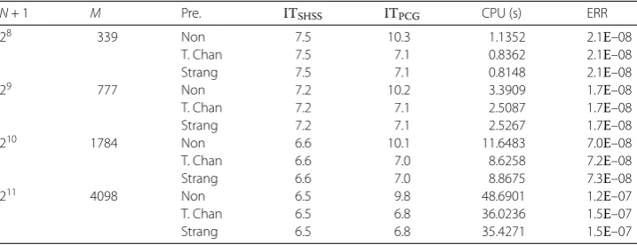
In the implementations, we adopt the experimentally optimal parameterβ= 0.01 for the SHSS-PCG iteration. Numerical results are given in Tables1–3. In these tables, we use “Non” for non-preconditioned method, “T. Chan” for T. Chan’s circulant preconditioner, and “Strang” for Strang’s circulant preconditioner. “N” denotes the number of spatial grid points, “M=((N+ 1)αTv
N,M)/(xR–xL)α” denotes the number of time steps and taking
vN,M= 1, “ERR” denotes the error between the true solution and the approximation under
the infinity norm, “CPU (s)” denotes the total CPU time in seconds, and “IT” denotes the average number of iterations required for solving the FDE, i.e., IT = M1 Mm=1iter(m), where iter(m) denotes the number of iterations required for solving the linear systems.
Table 1 Numerical results of the SHSS-PCG method for solving FDE (α= 1.2)
N+ 1 M Pre. ITSHSS ITPCG CPU (s) ERR
28 339 Non 7.5 10.3 1.1352 2.1E–08
T. Chan 7.5 7.1 0.8362 2.1E–08
Strang 7.5 7.1 0.8148 2.1E–08
29 777 Non 7.2 10.2 3.3909 1.7E–08
T. Chan 7.2 7.1 2.5087 1.7E–08
Strang 7.2 7.1 2.5267 1.7E–08
210 1784 Non 6.6 10.1 11.6483 7.0E–08
T. Chan 6.6 7.0 8.6258 7.2E–08
Strang 6.6 7.0 8.8675 7.3E–08
211 4098 Non 6.5 9.8 48.6901 1.2E–07
T. Chan 6.5 6.8 36.0236 1.5E–07
Table 2 Numerical results of the SHSS-PCG method for solving FDE (α= 1.5)
N+ 1 M Pre. ITSHSS ITPCG CPU (s) ERR
28 1456 Non 5.1 10.8 3.4127 1.8E–08
T. Chan 5.1 7.2 2.4424 1.8E–08
Strang 5.1 7.3 2.4540 1.8E–08
29 4108 Non 4.9 10.3 13.2000 6.3E–08
T. Chan 4.9 6.9 10.5790 6.2E–08
Strang 4.9 6.9 9.1063 6.2E–08
210 11,602 Non 4.9 9.9 54.7901 2.7E–07
T. Chan 4.9 6.4 38.3217 2.6E–07
Strang 4.9 6.4 39.2306 2.6E–07
211 32,792 Non 4.1 9.0 222.3530 8.5E–06
T. Chan 4.1 5.4 158.7036 7.8E–06
Strang 4.1 5.4 151.6013 7.8E–06
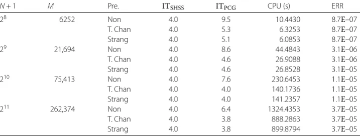
Table 3 Numerical results of the SHSS-PCG method for solving FDE (α= 1.8)
N+ 1 M Pre. ITSHSS ITPCG CPU (s) ERR
28 6252 Non 4.0 9.5 10.4430 8.7E–07
T. Chan 4.0 5.3 6.3253 8.7E–07
Strang 4.0 5.1 6.0853 8.7E–07
29 21,694 Non 4.0 8.6 44.4843 3.1E–06
T. Chan 4.0 4.6 26.9088 3.1E–06
Strang 4.0 4.6 26.8528 3.1E–05
210 75,413 Non 4.0 7.6 230.6453 1.1E–05
T. Chan 4.0 4.0 140.1736 1.1E–05
Strang 4.0 4.0 141.2357 1.1E–05
211 262,374 Non 4.0 6.4 1324.4353 3.7E–05
T. Chan 4.0 3.8 888.2863 3.7E–05
Strang 4.0 3.8 899.8794 3.7E–05
From these tables, one can see that all experimented methods can successfully produce approximate solution to the full non-symmetric linear systems. WhenN increases, the number of iteration steps is either fixed or decreases slightly, but the amount of total CPU times increases. When the order of fractional derivativeαbecomes large, the number of iteration steps decreases slightly, but the amount of CPU time increases significantly.
Further, with two classic circulant preconditioners, the number of iterations and the amount of CPU time decrease rapidly, and are half of those of the SHSS-PCG method with non-preconditioner.
We must note that the efficiency of preconditioners employed in the proposed PCG method is lower. The reason is that the number of inner iterations in the SHSS-PCG is small, which means that there is not enough space to improve the efficiency of preconditioner for the SHSS-PCG method.
6 Concluding remarks
Acknowledgements
Not applicable.
Funding
The research was supported by the National Natural Science Foundation of China (Grants Nos. 11661033, 11771193) and the Scientific Research Foundation for Doctor of Hexi University.
Availability of data and materials
Not applicable.
Competing interests
The authors declare that they have no competing interests.
Authors’ contributions
All three authors read and approved the final version of the manuscript.
Author details
1School of Mathematics and Statistics, Hexi University, Zhangye, China.2School of Mathematics and Statistics, Lanzhou
University, Lanzhou, China.3College of Chemistry and Chemical Engineering, Hexi University, Zhangye, China.
Publisher’s Note
Springer Nature remains neutral with regard to jurisdictional claims in published maps and institutional affiliations.
Received: 22 March 2019 Accepted: 25 September 2019 References
1. Tariboon, J., Ntouyas, S.K., Agarwal, P.: New concepts of fractional quantum calculus and applications to impulsive fractionalq-difference equations. Adv. Differ. Equ.201518 (2015)
2. Ruzhansky, M., Cho, Y.J., Agarwal, P., et al.: Advances in Real and Complex Analysis with Applications. Springer, Singapore (2017)
3. Kumar, D., Singh, J., Baleanu, D., et al.: Analysis of a fractional model of the Ambartsumian equation. Eur. Phys. J. Plus
133(7), 259 (2018)
4. Baleanu, D., Jajarmi, A., Asad, J.H.: Classical and fractional aspects of two coupled pendulums. Rom. Rep. Phys.71(1), 103 (2019)
5. Kumar, D., Tchier, F., Singh, J., et al.: An efficient computational technique for fractal vehicular traffic flow. Entropy
20(4), 259 (2018)
6. Benson, D.A., Wheatcraft, S.W., Meerschaert, M.M.: The fractional-order governing equation of Lévy motion. Water Resour. Res.36(6), 1413–1423 (2000)
7. Benson, D.A., Wheatcraft, S.W., Meerschaert, M.M.: Application of a fractional advection-dispersion equation. Water Resour. Res.36(6), 1403–1412 (2000)
8. Shlesinger, M.F., West, B.J., Klafter, J.: Lévy dynamics of enhanced diffusion: application to turbulence. Phys. Rev. Lett.
58(11), 1100–1103 (1987)
9. Carreras, B.A., Lynch, V.E., Zaslavsky, G.M.: Anomalous diffusion and exit time distribution of particle tracers in plasma turbulence model. Phys. Plasmas8(12), 5096–5103 (2001)
10. Magin, R.L.: Fractional Calculus in Bioengineering, vol. 149. Begell House Publishers, Redding (2006) 11. Bai, J., Feng, X.-C.: Fractional-order anisotropic diffusion for image denoising. IEEE Trans. Image Process.16(10),
2492–2502 (2007)
12. Jagdev, S., Aydin, S., Ram, S., et al.: A reliable analytical approach for a fractional model of advection-dispersion equation. Nonlinear Eng.9, 107–116 (2019)
13. Goswami, A., Singh, J., Kumar, D.: An efficient analytical approach for fractional equal width equations describing hydro-magnetic waves in cold plasma. Physica A524, 563–575 (2019)
14. Meng, R., Yin, D., Corina, S.D.: Variable-order fractional description of compression deformation of amorphous glassy polymers. Comput. Mech.64(1), 163–171 (2019)
15. Baleanu, D., Sadat Sajjadi, S., Jajarmi, A.: New features of the fractional Euler–Lagrange equations for a physical system within non-singular derivative operator. Eur. Phys. J. Plus134(4), 181 (2019)
16. Zhou, H., Agarwal, P.: Existence of almost periodic solution for neutral Nicholson blowflies model. Adv. Differ. Equ.
2017(1), 329 (2017)
17. Saoudi, K., Agarwal, P., Kumam, P., et al.: The Nehari manifold for a boundary value problem involving Riemann–Liouville fractional derivative. Adv. Differ. Equ.2018, 263 (2018)
18. Morales-Delgado, V.F., Gómez-Aguilar, J.F., Saad, K.M., et al.: Analytic solution for oxygen diffusion from capillary to tissues involving external force effects: a fractional calculus approach. Physica A523, 48–65 (2019)
19. Hajipour, M., Jajarmi, A., Baleanu, D., et al.: On an accurate discretization of a variable-order fractional reaction-diffusion equation. Commun. Nonlinear Sci. Numer. Simul.69, 119–133 (2019)
20. Meerschaert, M.M., Scheffler, H.P., Tadjeran, C.: Finite difference methods for two-dimensional fractional dispersion equation. J. Comput. Phys.211(1), 249–261 (2006)
21. Murio, D.A.: Implicit finite difference approximation for time fractional diffusion equations. Comput. Math. Appl.56(4), 1138–1145 (2008)
22. Langlands, T.A.M., Henry, B.I.: The accuracy and stability of an implicit solution method for the fractional diffusion equation. J. Comput. Phys.205(2), 719–736 (2005)
24. Ervin, V.J., Heuer, N., Roop, J.P.: Numerical approximation of a time dependent, nonlinear, space-fractional diffusion equation. SIAM J. Numer. Anal.45(2), 572–591 (2007)
25. Xu, Q.-W., Hesthaven, J.S.: Discontinuous Galerkin method for fractional convection-diffusion equations. SIAM J. Numer. Anal.52(1), 405–423 (2014)
26. Deng, W.-H., Hesthaven, J.S.: Local discontinuous Galerkin methods for fractional diffusion equations. ESAIM: Math. Model. Numer. Anal.47(06), 1845–1864 (2013)
27. Singh, J., Kumar, D., Baleanu, D., et al.: An efficient numerical algorithm for the fractional Drinfeld–Sokolov–Wilson equation. Appl. Math. Comput.335, 12–24 (2018)
28. Chen, C.M., Liu, F.-W., Turner, I., Anh, V.: A Fourier method for the fractional diffusion equation describing sub-diffusion. J. Comput. Phys.227(2), 886–897 (2007)
29. Piret, C., Hanert, E.: A radial basis functions method for fractional diffusion equations. J. Comput. Phys.238, 71–81 (2013)
30. Meerschaert, M.M., Tadjeran, C.: Finite difference approximations for two-sided space-fractional partial differential equations. Appl. Numer. Math.56(1), 80–90 (2006)
31. Meerschaert, M.M., Tadjeran, C.: Finite difference approximations for fractional advection-dispersion flow equations. J. Comput. Appl. Math.172(1), 65–77 (2004)
32. Wang, H., Wang, K.-X., Sircar, T.: A directo(nlog 2n) finite difference method for fractional diffusion equations. J. Comput. Phys.229(21), 8095–8104 (2010)
33. Wang, H., Wang, K.-X.: Ano(nlog 2n) alternating-direction finite difference method for two-dimensional fractional diffusion equations. J. Comput. Phys.230(21), 7830–7839 (2011)
34. Ng, M.K.: Iterative Methods for Toeplitz Systems. Oxford University Press, New York (2004)
35. Chan, R.H., Ng, M.K.: Conjugate gradient methods for Toeplitz systems. SIAM Rev.38(3), 427–482 (1996) 36. Chan, R.H., Jin, X.-Q.: An Introduction to Iterative Toeplitz Solvers, vol. 5. SIAM, Philadelphia (2007)
37. Wang, K.-X., Wang, H.: A fast characteristic finite difference method for fractional advection-diffusion equations. Adv. Water Resour.34(7), 810–816 (2011)
38. Lei, S.-L., Sun, H.-W.: A circulant preconditioner for fractional diffusion equations. J. Comput. Phys.242, 715–725 (2013) 39. Bai, Y.-Q., Huang, T.-Z., Gu, X.-M.: Circulant preconditioned iterations for fractional diffusion equations based on
Hermitian and skew-Hermitian splittings. Appl. Math. Lett.48, 14–22 (2015)
40. Li, C.-X., Wu, S.-L.: A single-step HSS method for non-Hermitian positive definite linear systems. Appl. Math. Lett.44, 26–29 (2015)
41. Strang, G.: A proposal for Toeplitz matrix calculations. Stud. Appl. Math.74(2), 171–176 (1986)