R E S E A R C H
Open Access
Discrete monotone method for
space-fractional nonlinear reaction–diffusion
equations
Salvador Flores
1, Jorge E. Macías-Díaz
1*and Ahmed S. Hendy
2,3*Correspondence:
1Departamento de Matemáticas y
Física, Universidad Autónoma de Aguascalientes, Aguascalientes, Mexico
Full list of author information is available at the end of the article
Abstract
A discrete monotone iterative method is reported here to solve a space-fractional nonlinear diffusion–reaction equation. More precisely, we propose a Crank–Nicolson discretization of a reaction–diffusion system with fractional spatial derivative of the Riesz type. The finite-difference scheme is based on the use of fractional-order centered differences, and it is solved using a monotone iterative technique. The existence and uniqueness of solutions of the numerical model are analyzed using this approach, along with the technique of upper and lower solutions. This methodology is employed also to prove the main numerical properties of the technique, namely, the consistency, stability, and convergence. As an application, the particular case of the space-fractional Fisher’s equation is theoretically analyzed in full detail. In that case, the monotone iterative method guarantees the preservation of the positivity and the boundedness of the numerical approximations. Various numerical examples are provided to illustrate the validity of the numerical approximations. More precisely, we provide an extensive series of comparisons against other numerical methods available in the literature, we show detailed numerical analyses of convergence in time and in space against fractional and integer-order models, and we provide studies on the robustness and the numerical performance of the discrete monotone method.
MSC: Primary 65M06; secondary 35K15; 35K55; 35K57
Keywords: Space-fractional diffusion–reaction equations; Crank–Nicolson finite-difference scheme; Discrete monotone iterative method; Existence and uniqueness of solutions; Numerical efficiency analysis
1 Introduction
Monotone iterative methods have been used in the literature to investigate differential equations (ordinary or partial) from both the analytical and numerical points of view. For example, from the analytical side, such iterative techniques have been applied to in-vestigate the existence and uniqueness of solutions of a wide range of parabolic partial differential equations [1], as well as other analytical features of the solutions. In par-ticular, this approach has been used to establish the existence of positive solutions of quasilinear parabolic systems with Dirichlet boundary conditions [2], to study quasilinear parabolic and elliptic systems with mixed quasimonotone functions [3], to analyze peri-odic boundary-value problems for differential equations with delay [4], to solve first-order
functional-difference equations with nonlinear boundary value conditions [5], to prove the existence and asymptotic behavior of solutions for quasilinear parabolic systems [6], and, recently, to establish the existence, uniqueness, and stability of the solutions of a parabolic model in the formation of porous silicon [7], among other interesting applications.
From the numerical point of view, monotone iterative methods have been also employed to effectively solve systems consisting of differential equations. As for the continuous case, the numerical monotone iterative methods require the knowledge of upper and lower so-lutions in order to generate two monotone sequences that converge to the solution of the problems under investigation. Numerical techniques of this nature have been employed to solve the multidimensional semiconductor Poisson equation [8], to simulate quantum-corrected energy transport models [9], to study numerically the solutions of parabolic problems with time delays [10], to investigate two-dimensional simulation of submicron MOSFETs [11], to provide numerical analysis of coupled systems of nonlinear parabolic equations [12], and to simulate porous silicon morphologies [13]. In various of these re-ports and many other articles which employ discrete monotone iterative approaches, this methodology has been used to prove the existence and uniqueness of solutions, as well as to investigate the numerical efficiency of the computational algorithms.
In summary, the monotone method has been extensively employed in the analysis and simulation of nonlinear systems of parabolic differential equations. Moreover, this method has been extended to investigate fractional systems of differential equations. Indeed, in recent years, fractional calculus has found a wide range of applications to viscoelasticity [14], the discretization of nonsingular Mittag-Leffler kernels [15], and fractional operators with exponential kernels and a Lyapunov type inequality [16] among other problems. Fur-thermore, it has been proved that some families of equations with long-range interactions lead to models governed by fractional differential equations in the continuous limit [17,
18]. In summary, fractional calculus has experienced fast development in the last years, and the development of monotone iterative techniques has seen continuous development within that area of research. However, many interesting problems still remain open to this day. One of them is the development of discrete monotone iterative methods to solve space-fractional diffusion–reaction regimes that generalize the well-known Fisher’s equa-tion [19,20]. This model is the simplest diffusive model with nonlinear reaction, and its many generalizations have been a highly transited avenue of research in mathematics and numerical analysis.
dif-fusion equations with Caputo fractional derivatives in time [28,29]. However, the Riesz space-fractional scenario has been left without study, perhaps in light of the difficulties arising in such a case.
The novelty of the present work lies in the fact that a monotone iterative method will be proposed for the first time in the literature to solve parabolic partial differential equations with Riesz fractional diffusion. We consider in this case a nonlinear reaction term, so that the mathematical model under investigation is a fractional extension of the well-known Fisher’s equation from population dynamics. Suitable initial-boundary conditions will be imposed on a closed and bounded interval of the real numbers. In a first step, we will pro-pose a Crank–Nicolson discretization of the fractional system, and a monotone iterative method will be proposed to solve the discretized model. Existence and uniqueness of so-lutions will hinge on the fact that the discrete model can be rewritten in vector form, and that the associated coefficient matrix is anM-matrix [30]. Moreover, the consistency, sta-bility and quadratic convergence of the technique will be mathematically proved using the monotone iterative approach, by imposing suitable computational requirements. A par-ticularly meaningful form of the fractional model will be investigated mathematically in deeper detail, and conditions for the existence, uniqueness, and numerical efficiency of the discrete solutions will be derived in that particular case.
This manuscript is organized as follows. In Sect.2, we introduce the fractional diffu-sive problem on interest and provide a Crank–Nicolson discretization based on the use of fractional-order centered differences. Here, it is worthwhile to recall that fractional-order centered differences have been used successfully by some of the authors in the discretiza-tion of various fracdiscretiza-tional problems [31–33]. Suitable discrete nomenclature is introduced to that end, including some helpful properties of the fractional centered differences and a convenient vector representation of the numerical model. Section3is devoted to present the discrete monotone method for the numerical method of this work. The existence and uniqueness of solutions of the iterative method are thoroughly proved in that stage. The most important numerical properties of the methodology are established in Sect.4, while Sect.5is devoted to theoretically analyze the numerical methodology for the fractional Fisher’s equation. Also, we provide thorough numerical comparisons of our methodol-ogy against various other approaches proposed in the literature. In particular, we show detailed numerical analyses of convergence in time and in space against fractional and integer-order models, and we provide studies on the robustness and numerical perfor-mance of the discrete monotone method. Section6is devoted to discuss the findings of this work. Finally, we close this manuscript with a section of concluding remarks.
2 Preliminaries
Throughout this work, we letL,T ∈R+andα∈(0, 1)∪(1, 2]. Consider an open spatial
domainΩ= (0,L)⊆R, and define the setΩT=Ω×(0,T). In this manuscript, we let
v:ΩT→Rbe a sufficiently differentiable function. Definevas zero outside ofΩT, and
we suppose that it satisfies the initial-boundary-value problem
∂v(x,t)
∂t –K
∂αv(x,t)
∂|x|α =f
x,t,v(x,t), ∀(x,t)∈ΩT,
such that
⎧ ⎨ ⎩
v(x, 0) =v0(x), ∀x∈Ω,
The fractional derivative in (1) is understood here in the Riesz sense, that is, we let
∂αv(x,t)
∂|x|α = –
1 2cos(απ
2 )Γ(2 –α)
∂2 ∂x2
∞
–∞
v(t,ξ)dξ
|x–ξ|α–1, ∀(x,t)∈ΩT. (2)
Here,Γ is the usual Gamma function andv0:Ω→Ris sufficiently smooth.
Definition 1 A functionv˜∈C2,1(Ω
T)∩C(ΩT) is calledan upper solutionof (1) if it solves
the problem
∂v˜(x,t)
∂t –K
∂αv˜(x,t)
∂|x|α ≥f
x,t,˜v(x,t), ∀(x,t)∈ΩT,
such that
⎧ ⎨ ⎩
˜
v(x, 0)≥v0(x), ∀x∈Ω, ˜
v(x,t)≥0, ∀(x,t)∈∂Ω×[0,T]. (3)
Similarly, we say that a functionvˆ∈C2,1(Ω
T)∩C(ΩT) isa lower solutionof (1) if it
sat-isfies (3) with all the inequalities reversed. Ifv˜andvˆare, respectively, upper and lower solutions of (1) then we will assume that they areordered, that is, they satisfyˆv≤ ˜v. With this nomenclature, we will suppose thatf :R3→Ris continuously differentiable, and that
there are suitable bounded functionsc≡c(x,t) andc≡c(x,t) such that
–c(x,t)(v1–v2)≤f(x,t,v1) –f(x,t,v2)≤c(x,t)(v1–v2), (4)
for allvˆ≤v2≤v1≤ ˜vand (x,t)∈ΩT.
For convenience, we letIP={1, . . . ,P}andIP=IP∪{0}, for eachP∈N. LetM,N∈Z, and
consider a grid ofΩTusing uniform spatial and temporal nodes of the formsxi=ihand
tk=kτ, respectively, for eachi∈IMandk∈IN. The spatial and temporal partition norms
areh=L/Mandτ =T/N, respectively, and we use the symbolsvki andVik, respectively, to represent the exact and numerical solutions of (1) at (xi,tk). In this work, the temporal
partial derivative of (1) will be calculated through the forward-difference scheme
∂v(xi,tk)
∂t = vk+1
i –vki
τ +O(τ), ∀(i,k)∈IM–1×IN–1. (5) Definition 2(Ortigueira [34]) For any functionϕ:R→R,h> 0 andα> –1 we define the
fractional centered differenceof orderαofϕat the pointxas
αhϕ(x) =
∞
m=–∞
gmαϕ(x–mh), ∀x∈R, (6)
whenever the right-hand side of this expression converges. The coefficients (gα
k)∞k=–∞are
defined by
gmα = (–1)
mΓ(α+ 1)
Lemma 3(Wang et al. [27]) Ifα∈(0, 1)∪(1, 2]then the coefficients(7)satisfy the following
As a consequence of this lemma, the series in the right-hand side of (6) converges ab-solutely for any bounded functionϕ∈L1(R). With this notation, it is easy to see that any
ϕ∈C5(R), for which all of its derivatives up to order five belong toL1(R), has the property
In this work, we use formulas (5) and (9) in order to propose the following scheme to solve (1):
It is obvious that this numerical model is a Crank–Nicolson-type of scheme. For the sake of convenience, we letr=12τh–α, and define the (M+ 1)-dimensional real vectors
Using this nomenclature, system (11) can be readily rewritten in vector form as
3 Discrete monotone method
The purpose of the present section is to introduce a discrete monotone method, and use it to establish the existence and uniqueness of the solutions of the discrete system (14). In the following, given any real vectorsVandWof the same dimensions, we will employ the notationV≤W(alternatively,W≥V) meaning that each component ofVis less than or equal to the corresponding component ofW.
Letc(x,t) andc(x,t) be bounded functions satisfying the requirements in Definition1.
have omitted the dependence ofCandConkfor the sake of convenience. Note that (4) implies thatF(Vk) is nondecreasing. Using Picard iterations, we reach the iterative system
⎧
ordered upper and lower solutions of (14), in the sense of Definition4below. In the sequel, system (17) will be referred to simply as thediscrete monotone(DM) method.
Definition 4 The (M+ 1)-dimensional real vectorV˜k is anupper solutionof (14) if it
Similarly, the real vectorVˆkis alower solutionof (14) if it satisfies all the reversed
inequal-ities in (18). If{ ˜Vk}Nk=0 and{ ˆVk}Nk=0are respectively sets of upper and lower solutions of
(14), we will assume tacitly that they areordered, that is,V˜k≥ ˆVkfor allk∈IN–1.
Definition 5 A square real matrixAis anM-matrixif there exist a nonnegative matrixB
and a numberμ≥ρ(B) such thatAcan be expressed in the formA=μI–B. Here,ρ(B) represents the spectral radius ofB.
It is important to recall thatM-matrices are nonsingular, and their inverses are nonneg-ative matrices.
Theorem 6(Plemmons [35]) A square real matrix A is an M-matrix if and only if
(ii) all its off-diagonal components are nonpositive,and
(iii) there exists a diagonal matrixDwith positive diagonal entries such thatADis strictly diagonally dominant.
The hypothesis (19) and Lemma3guarantee then that (i) of Theorem6is satisfied. On the other hand, note that the off-diagonal elementsξr,sofΞ are the constantsgkα, for suitable
indexesk∈Z\ {0}, whence condition (ii) of Theorem6holds. Finally, (19) assures thatΞ
is already diagonally dominant in view of
M
The conclusion of the theorem readily follows now from Theorem6.
Theorem 8(Existence and uniqueness) LetV˜k andVˆk be respectively upper and lower
solutions of (14)at time tk,for each k∈IN.Define the constant
is satisfied then these sequences have the property that
ˆ
Moreover,the sequences converge to the unique solution of(14)between its upper and lower solutions.
Proof We will prove the theorem in three steps. Firstly, we will show inductively that (23) is satisfied, for eachk∈IN andp∈N∪ {0}. Secondly, we will prove that the sequences
converge to the solution of (14) and, finally, we will establish the existence and uniqueness of solutions as a direct consequence of the first and second steps.
We subtract then inequality (24) from the following equation that results from (17):
k are also satisfied. In summary, we have
established so far thatW(1)k ≥0, for eachk∈IN.
k . An inductive argument overkand reuse of the arguments
employed above leads toW(kp+1+1)≥0andV(kp+1)≥V(kp). The proofs thatV(kp)≥V(kp+1)
k . We have established thus the validity of the chain of inequalities
(23).
2. Expression (23) implies that{V(kp)}∞p=0is nonincreasing and bounded from below, while{V(kp)}∞p=0is nondecreasing and bounded from above. This implies that the following limits exist for eachk∈IN:
lim
we know that the matrixI–rQis positive. Therefore, we reach
Wk+1≤(I+rQ)–1(I–rQ)Wkin light that each solution of (14) satisfies the initial
condition, that is,V0=V0∗. It follows thatW1≤0and, using induction overk, we
obtain thatWk≤0andVk=Vk∗. The proof thatVk∗=Vkis analogous, letting
3. Finally, the construction of the sequence{Vk}can be readily established using
induction overk. The approximationV0is defined through the initial condition.
Supposing thatVkhas been already obtained,Vk+1is reached using the iterative
technique and the approximationVk.
4 Numerical efficiency
In this stage, we establish the main numerical properties of the DM method, namely, the consistency, stability and convergence. In our proofs, we will require that the conditions of Theorem8are satisfied in order to guarantee the existence and uniqueness of the solutions of the DM method.
Definition 9 Let{Yk} and{Yk} be sequences of approximations to the solution of the
problemAy= 0, obtained by using the schemeAyk= 0 with the initial conditionsY0and Y0, respectively. The difference scheme isstableif givenε> 0 there existsδ> 0 such that
Yk–Yk<εfor allk∈IN, wheneverY0–Y0 ≤δ.
We will need the following result to prove the stability of method (14).
Lemma 10(Flores and Jerez [13]) Let{Yk(r+1)}be a sequence of vectors withY0(r),Yk(0) ≤
δ,such that
Yk(r+1)≤a1Yk(r)+a2Yk(r+1–1)+a3Yk(r–1), (31)
where a1,a2and a3are positive constants with a1< 1.Then,for all k∈IR,
Yk(r+1)≤ϑr+ (1 +a3)ϑr+ϑr–1+· · ·+ϑ+ 1δ, (32)
whereϑ=a2+a3 1–a1 .
Theorem 11 The DM method is unconditionally stable if (22)is satisfied.
Proof Suppose thatδ> 0, and letZk(p)be a perturbation ofVk(p)orV(kp), with the property thatZ0(p)–V(0p)<δandZk(0)–V(0)k <δ. Suppose thatZk(p)satisfies
BZk(p+1) =DZk(p)+rhαFZ(p–1)
k+1
+FZk(p–1). (33)
DefineYk(p)=Zk(p)–V(kp), soY0(p)<δandYk(0)<δ. Subtracting (17) from (33), we obtain
BYk(p+1) =DYk(p)+rhαFZk(p+1–1)–FVk(p+1–1) +rhαFZ(p–1)
k
–FVk(p–1) (34)
and
Y(p)
k+1≤a1Y (p)
k +a2Y
(p–1)
k+1 +a3Y (p–1)
k , (35)
wherea1=B–1D,a2=rhαB–1C, anda3=rhαB–1C. Notice that
Finally, inequality (32) follows by Lemma10. We conclude that method (17) is
uncondi-tionally stable.
In the previous section, we showed the DM method (17) converges to a unique solution of the discrete system (14). We will prove now that the DM method (17) converges also the solution of the continuous problem (1).
Theorem 12(Consistency) If v(x,t)∈C5,2(Ω
T)and f is continuously differentiable then
the discrete scheme(14)is consistent with equation(1).
Proof Letφandψbe the exact and approximation operators, respectively, corresponding to equation (1). Obviously, these operators satisfy
φik=∂v
consistency properties of the individual discrete operators and Taylor’s theorem, there exist positive constantsC1,C2, andC3such that
consistency of (14) readily follows.
Finally, we prove the convergence of the discrete method.
Theorem 13(Convergence) Let v(x,t)∈C5,2(Ω
T),and let f be continuously differentiable.
If f satisfies(4)and the hypotheses of Theorem(8)hold then the DM method(17)converges to the unique solution of equation(1).
It only remains to show that the solutions of the discrete system (14) converge to those of the continuous, that is,
lim
τ,h→0+Vk–Wk= 0, ∀k∈IN. (42)
To that end, letVk= (vk0,vk1, . . . ,vkM) andWk= (wk0,wk1, . . . ,wkM). Using Lemma12, the
dis-crete system (14), hypotheses of this theorem, and matrixC, we obtain that
(I+rKA)(Vk+1–Wk+1) +O
τ+h2
= (I–rKA)(Vk–Wk) +rhα
F(Vk+1) –F(Wk+1) +F(Vk) –F(Wk)
≤(I–rKA)(Vk–Wk) +rhαC[Vk+1–Wk+1] +rhαC[Vk–Wk], (43)
for eachk∈IN–1. Then [I+rQ](Vk+1–Wk+1)≤[I–rQ](Vk–Wk) +O(τ +h2), where
Q=KA–hαC. Now, inequality (22) guarantees that theI+rQis positive. This implies
that
Vk+1–Wk+1 ≤ ΛVk–Wk+ΘO
τ+h2, ∀k∈IN–1, (44)
whereΛ= [I+rQ]–1[I–rQ] andΘ= [I+rQ]–1. Using induction, we obtain
Vk–Wk ≤ ΛkV0–W0+ΘΛk–1O
τ+h2, ∀k∈IN–1. (45)
The limit (42) is readily established now from the facts thatΛ< 1 andΘ< 1. This
completes the proof.
5 Numerical examples
In this section, we describe the computational implementation of the DM method to solve Fisher’s equation with fractional diffusion. More concretely, we will consider the problem
∂v(x,t)
∂t –K
∂αv(x,t)
∂|x|α =v(x,t)
1 –v(x,t), ∀(x,t)∈ΩT,
such that
⎧ ⎨ ⎩
v(x, 0) =v0(x), ∀x∈Ω,
v(x,t) = 0, ∀(x,t)∈∂Ω×[0,T]. (46)
To that end, note that condition (4) requires for the functionsc(x,t) andc(x,t) to be cal-culated as
c(x,t) =sup
–∂f(v)
∂v :vˆ≤v≤ ˜v
, (47)
c(x,t) =sup
∂f(v)
∂v :vˆ≤v≤ ˜v
. (48)
From equation (46), it follows that c(x,t) = c(x,t) =η =max{2γ – 1, 1}, where γ =
max{1,maxΩv0(x)}. Using the uniform grid introduced in Sect.2along with the matrix
system (17), it follows that
with
is clear that theV˜ satisfies the inequality
1 +γrK1
Using the upper and lower solutions provided in Lemma14, our implementation of the DM method will make use of the iterative system
⎧
Lemma 15 Suppose that the following condition is satisfied:
Then the sequences{V(kp)}and{V(kp)}obtained by(55)converge to the unique solution of
(46)betweenVˆkandV˜k.
Proof The proof follows from Theorem8.
The following is a trivial consequence of the previous lemma.
Theorem 16(Positivity and boundedness) Suppose that condition(56)is satisfied.Then
the discrete model (46)is capable of preserving the positivity and the boundedness from above by1of the numerical approximations.
Next, we provide some computational simulations to confirm the validity of the approx-imations obtained through the DM method. In view of the lack of known exact solutions for the fully fractional model considered in this work, we compare our results with those of other techniques available in the literature. Beforehand, we must mention that our compu-tational implementation of the DM monotone method will hinge on the use of lower and upper solutions for the problem under investigation. They will be used as starting approx-imations at each iteration in order to generate the sequences (23). As stopping criterion, we will set a maximum difference in the infinity norm equal to 1×10⁻¹⁰or a maximum
number of iterations equal to 20. It is important to point out that this maximum number of iterations was never reached in our simulations. In fact, the maximum error was obtained usually in 8 iterations of the DM method.
Example17 LetΩ= (0,π) andT= 1, and we will consider the problem
∂v(x,t)
∂t –K
∂αv(x,t)
∂|x|α =sin
v(x,t), ∀(x,t)∈ΩT,
such that
⎧ ⎨ ⎩
v(x, 0) =sinx, ∀x∈Ω,
v(x,t) = 0, ∀(x,t)∈∂Ω×[0, 1]. (57)
For convenience, we letK= 0.1. Computationally, we fix the parametersh=π/200 and
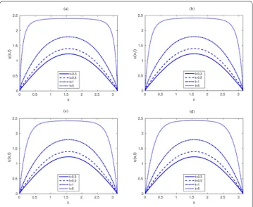
Figure 1Approximate solution of the problem (57) using the DM method, at the timest= 0.3 (solid), 0.5 (dashed), 1 (dashed–dotted) and 5 (dotted). Various values ofαwere used, namely, (a)α= 1.2, (b)α= 1.4, (c) α= 1.6, and (d)α= 1.8. The solutions were calculated overΩ= (0,π), and usingK= 0.1. Computationally, we leth=π/200 andτ= 0.016
Next, we will perform an analysis of convergence of the DM method, considering nor-mal diffusion and long times. To that end, we will consider problem (46) withK= 1, and employ the exact traveling-wave solution
v(x,t) =
1 +Cexp
1 √
6x– 5 6t
–2
, ∀(x,t)∈R×R+. (58)
In our simulations, we will modify the methodology proposed in this work to account for exact Dirichlet boundary conditions, prescribing them through (58). Moreover, we will employ the maximum-norm error between the exact solution of (46) at the timeT, and the corresponding numerical solution calculated using the DM method, namely,
τ,h=max!v(xi,tK) –ViK:i∈IM
"
. (59)
We also define the following standard rates:
ρτ =log2
2τ,h
τ,h
, ρh=log2
τ,2h
τ,h
. (60)
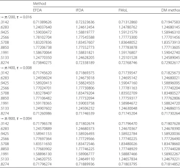
Table 1 Values of the approximate solution of problem (57) at different values ofxandT= 0.3, using Ω= (0,π),α= 1.8, andK= 0.1. Computationally, we used different combinations of values ofhand τ. The results were obtained using the EFDA, IFDA, and FMoL reported in [36], as well as the DM method introduced in the present manuscript
Method
x EFDA IFDA FMoL DM method
h=π/200,τ= 0.016
0.3142 0.40643185 0.40591753 0.40722026 0.40523810
0.6283 0.75093552 0.75000260 0.75219110 0.74870365
0.9425 1.01391315 1.01236366 1.01519975 1.01087353
1.2566 1.17543235 1.17356309 1.17739215 1.17196504
1.5708 1.22928866 1.22798315 1.23181079 1.22597857
1.8850 1.17482175 1.17399495 1.17730057 1.17196504
2.1991 1.01388718 1.01274958 1.01539033 1.01087353
2.5133 0.75121711 0.75012166 0.75238197 0.74870365
2.8274 0.40650703 0.40608269 0.40746642 0.40523810
h=π/400,τ= 0.008
0.3142 0.40798803 0.40800055 0.40803064 0.40790925
0.6283 0.75305289 0.75306981 0.75312693 0.75290589
0.9425 1.01613053 1.01613171 1.01623145 1.01593914
1.2566 1.17754898 1.17754418 1.17768450 1.17733677
1.5708 1.23163392 1.23163641 1.23173842 1.23140839
1.8850 1.17754907 1.17755395 1.17763565 1.17733677
2.1991 1.01614381 1.01611409 1.01622990 1.01593914
2.5133 0.75305404 0.75304748 0.75313106 0.75290589
2.8274 0.40798587 0.40798503 0.40803474 0.40790925
h=π/800,τ= 0.004
0.3142 0.40923740 0.40924090 0.40925669 0.40924443
0.6283 0.75497993 0.75499925 0.75502314 0.75500177
0.9425 1.01843426 1.01845552 1.01849042 1.01846144
1.2566 1.17998806 1.18000297 1.18004151 1.18000806
1.5708 1.23410056 1.23411599 1.23414084 1.23410729
1.8850 1.18000780 1.18001024 1.18003866 1.18000806
2.1991 1.01846042 1.01846591 1.01848874 1.01846144
2.5133 0.75499623 0.75500746 0.75502307 0.75500177
2.8274 0.40924316 0.4092445549 0.40925683 0.40924443
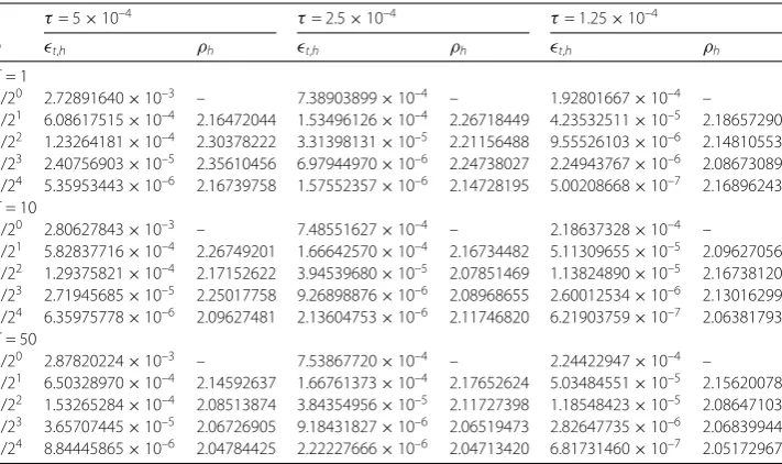
circumstances, Table4provides a temporal numerical convergence analysis of the DM method at various values ofT. The results confirm that the method possesses linear or-der of temporal convergence, in agreement with Theorem13. In turn, Table5shows the spatial convergence analysis of the DM method. Again, the results confirm the conclusion of Theorem13.
Finally, we compare the performance and the robustness of the methods used in Example
17using an exact solution for a fractional problem. To that end, we will follow closely the approach of [37] to prove the robustness of our the DM method. As in that work, we will consider the problem (1) defined overΩT= (0, 1)×(0, 1), and fix the reaction function as
f(x,t,v) = 3K 4
1 + (2π)αsin(2πx) –K 4
1 + (6π)αsin(6πx)
+αtα–1sin3(2πx) –Kv, ∀(x,t,v)∈ΩT×R. (61)
In this case, the exact solution of the problem forα∈(1, 2] is given by
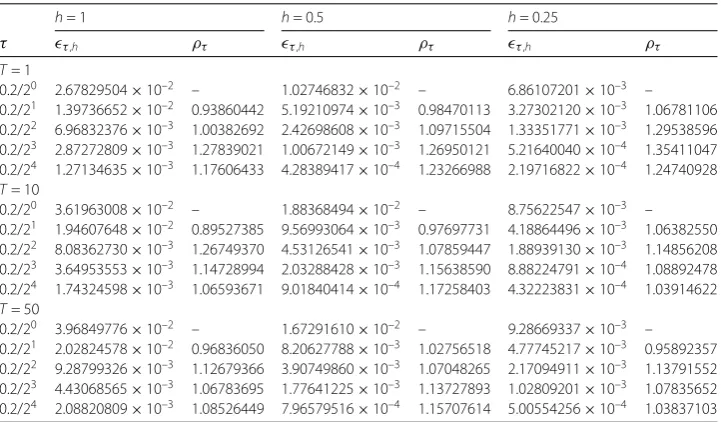
Table 2 Values of the approximate solution of problem (57) at different values ofxandT= 1, using Ω= (0,π),α= 1.8, andK= 0.1. Computationally, we used different combinations of values ofhand τ. The results were obtained using the EFDA, IFDA, and FMoL reported in [36], as well as the DM method introduced in the present manuscript
Method
x EFDA IFDA FMoL DM method
h=π/200,τ= 0.016
0.3142 0.71389626 0.72323636 0.71312860 0.71947583
0.6283 1.24037640 1.24612454 1.24780762 1.24680145
0.9425 1.59030472 1.58819777 1.59121579 1.58946310
1.2566 1.78102704 1.77545588 1.77773300 1.77701456
1.5708 1.83207836 1.83457607 1.83648052 1.83573913
1.8850 1.77206738 1.77552773 1.77783878 1.77713605
2.1991 1.58670064 1.58831821 1.59176807 1.59042740
2.5133 1.24770350 1.24628205 1.25101528 1.24589045
2.8274 0.73840275 0.72338189 0.72768746 0.72902617
h=π/400,τ= 0.008
0.3142 0.71745620 0.71869375 0.71739547 0.71825673
0.6283 1.24936024 1.24673018 1.24695142 1.24680021
0.9425 1.58920413 1.58824503 1.59047160 1.58896095
1.2566 1.77024701 1.77730806 1.77781163 1.77740204
1.5708 1.83278407 1.83479204 1.83502709 1.83480527
1.8850 1.77106482 1.77732094 1.77759317 1.77762806
2.1991 1.59178365 1.59003758 1.58984672 1.58824720
2.5133 1.24907602 1.24506232 1.24630048 1.24686015
2.8274 0.71260986 0.71746539 0.71745204 0.71730264
h=π/800,τ= 0.004
0.3142 0.71796578 0.71802674 0.71796470 0.71807628
0.6283 1.24570889 1.24680373 1.24670367 1.24678390
0.9425 1.58941153 1.58926493 1.58922784 1.58920036
1.2566 1.77697364 1.77729566 1.77740225 1.77726490
1.5708 1.83511650 1.83472546 1.83480026 1.83478660
1.8850 1.77683902 1.77746225 1.77748929 1.77744028
2.1991 1.58896130 1.58906777 1.58887466 1.58902267
2.5133 1.24620755 1.24649110 1.24657834 1.24679221
2.8274 0.71796274 0.71889936 0.71803795 0.71814852
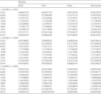
Example19 LetΩ = (0, 1),K= 0.1 and T = 1, and consider problem (1) with reaction function given by (61). For illustration purposes, Fig.2shows the approximation to the solutionv(x,t) of this problem as a function ofxandt. We used the DM method to produce the approximations, fixingh=τ= 0.01. Various values ofαwere employed, namely, (a)α= 1.01, (b)α= 1.2, (c)α= 1.4, (d)α= 1.6, (e)α= 1.8, and (f )α= 2. Figure3provides graphical summaries of the temporal convergence and efficiency analyses of the methods used in Example19. In these analyses, we employed the exact solution (62) of problem (1) with reaction function (61). The results show that the DM method is a first-order convergent technique in time, which yields smaller errors for fixed values ofτ. Moreover, the DM method is a more efficient technique according to out results. These results show that the DM method is a more efficient and robust technique than the EFDA, IFDA, and FMoL. It is worth pointing out that we also carried out analysis of spatial performance and robustness. The results (not shown here in view of the redundancy) yield the same conclusions on the DM method.
compu-Table 3 Values of the approximate solution of problem (57) at different values ofxandT= 3, using Ω= (0,π),α= 1.8, andK= 0.1. Computationally, we used different combinations of values ofhand τ. The results were obtained using the EFDA, IFDA, and FMoL reported in [36], as well as the DM method introduced in the present manuscript
Method
x EFDA IFDA FMoL DM method
h=π/200,τ= 0.016
0.3142 1.57368789 1.57372511 1.57392168 1.57372919
0.6283 2.16380277 2.16386523 2.16399150 2.16385886
0.9425 2.33655001 2.33663342 2.33667019 2.33661347
1.2566 2.38754579 2.38764530 2.38762011 2.38761337
1.5708 2.39918437 2.39929592 2.39922930 2.39925392
1.8850 2.38753659 2.38766383 2.38756809 2.38761337
2.1991 2.33650970 2.33667395 2.33654916 2.33661347
2.5133 2.16369084 2.16393561 2.16376674 2.16385886
2.8274 1.57350732 1.57381573 1.57361994 1.57372919
h=π/400,τ= 0.008
0.3142 1.57438633 1.57437820 1.57435879 1.57435676
0.6283 2.16341461 2.16340869 2.16339364 2.16339412
0.9425 2.33597962 2.33597699 2.33597013 2.33597013
1.2566 2.38702266 2.38702177 2.38701950 2.38701864
1.5708 2.39869212 2.39869098 2.39869138 2.39868980
1.8850 2.38702107 2.38701906 2.38702156 2.38701864
2.1991 2.33597346 2.33597038 2.33597368 2.33597013
2.5133 2.16339880 2.16339599 2.16339738 2.16339412
2.8274 1.57436187 1.57436096 1.57436143 1.57435676
h=π/800,τ= 0.004
0.3142 1.57400608 1.57400734 1.57400844 1.57400710
0.6283 2.16262828 2.16262984 2.16263132 2.16263025
0.9425 2.33531356 2.33531372 2.33531405 2.33531388
1.2566 2.38648630 2.38648729 2.38648785 2.38648734
1.5708 2.39820239 2.39820243 2.39820257 2.39820244
1.8850 2.38648651 2.38648731 2.38648785 2.38648734
2.1991 2.33531397 2.33531392 2.33531389 2.33531387
2.5133 2.16263007 2.16263026 2.16263073 2.16263025
2.8274 1.57400875 1.57400804 1.57400742 1.57400710
Table 4 Table of absolute errors in the maximum norm and temporal rates of convergence for various values of the parametersτandh. We usedf(u) =u(1 –u), and the exact solution (58) of model (46). We employed alsoΩ= (–200, 200) and various values ofT
h= 1 h= 0.5 h= 0.25
τ τ,h ρτ τ,h ρτ τ,h ρτ
T= 1
0.2/20 2.67829504×10⁻² – 1.02746832×10⁻² – 6.86107201×10⁻³ – 0.2/21 1.39736652×10⁻² 0.93860442 5.19210974×10⁻³ 0.98470113 3.27302120×10⁻³ 1.06781106 0.2/22 6.96832376×10⁻³ 1.00382692 2.42698608×10⁻³ 1.09715504 1.33351771×10⁻³ 1.29538596 0.2/23 2.87272809×10⁻³ 1.27839021 1.00672149×10⁻³ 1.26950121 5.21640040×10⁻⁴ 1.35411047 0.2/24 1.27134635×10⁻³ 1.17606433 4.28389417×10⁻⁴ 1.23266988 2.19716822×10⁻⁴ 1.24740928
T= 10
0.2/20 3.61963008×10⁻² – 1.88368494×10⁻² – 8.75622547×10⁻³ – 0.2/21 1.94607648×10⁻² 0.89527385 9.56993064×10⁻³ 0.97697731 4.18864496×10⁻³ 1.06382550 0.2/22 8.08362730×10⁻³ 1.26749370 4.53126541×10⁻³ 1.07859447 1.88939130×10⁻³ 1.14856208 0.2/23 3.64953553×10⁻³ 1.14728994 2.03288428×10⁻³ 1.15638590 8.88224791×10⁻⁴ 1.08892478 0.2/24 1.74324598×10⁻³ 1.06593671 9.01840414×10⁻⁴ 1.17258403 4.32223831×10⁻⁴ 1.03914622
T= 50
Table 5 Table of absolute errors in the maximum norm and spatial rates of convergence for various values of the parametersτ andh. We usedf(u) =u(1 –u), and the exact solution (58) of model (46). We employed alsoΩ= (–200, 200) and various values ofT
τ= 5×10⁻⁴ τ= 2.5×10⁻⁴ τ= 1.25×10⁻⁴
h t,h ρh t,h ρh t,h ρh
T= 1
2/20 2.72891640×10⁻³ – 7.38903899×10⁻⁴ – 1.92801667×10⁻⁴ – 2/21 6.08617515×10⁻⁴ 2.16472044 1.53496126×10⁻⁴ 2.26718449 4.23532511×10⁻⁵ 2.18657290 2/22 1.23264181×10⁻⁴ 2.30378222 3.31398131×10⁻⁵ 2.21156488 9.55526103×10⁻⁶ 2.14810553 2/23 2.40756903×10⁻⁵ 2.35610456 6.97944970×10⁻⁶ 2.24738027 2.24943767×10⁻⁶ 2.08673089 2/24 5.35953443×10⁻⁶ 2.16739758 1.57552357×10⁻⁶ 2.14728195 5.00208668×10⁻⁷ 2.16896243
T= 10
2/20 2.80627843×10⁻³ – 7.48551627×10⁻⁴ – 2.18637328×10⁻⁴ – 2/21 5.82837716×10⁻⁴ 2.26749201 1.66642570×10⁻⁴ 2.16734482 5.11309655×10⁻⁵ 2.09627056 2/22 1.29375821×10⁻⁴ 2.17152622 3.94539680×10⁻⁵ 2.07851469 1.13824890×10⁻⁵ 2.16738120 2/23 2.71945685×10⁻⁵ 2.25017758 9.26898876×10⁻⁶ 2.08968655 2.60012534×10⁻⁶ 2.13016299 2/24 6.35975778×10⁻⁶ 2.09627481 2.13604753×10⁻⁶ 2.11746820 6.21903759×10⁻⁷ 2.06381793
T= 50
2/20 2.87820224×10⁻³ – 7.53867720×10⁻⁴ – 2.24422947×10⁻⁴ – 2/21 6.50328970×10⁻⁴ 2.14592637 1.66761373×10⁻⁴ 2.17652624 5.03484551×10⁻⁵ 2.15620078 2/22 1.53265284×10⁻⁴ 2.08513874 3.84354956×10⁻⁵ 2.11727398 1.18548423×10⁻⁵ 2.08647103 2/23 3.65707445×10⁻⁵ 2.06726905 9.18431827×10⁻⁶ 2.06519473 2.82647735×10⁻⁶ 2.06839944 2/24 8.84445865×10⁻⁶ 2.04784425 2.22227666×10⁻⁶ 2.04713420 6.81731460×10⁻⁷ 2.05172967
tational times, we are aware that better results may be obtained with more modern equip-ment, more modest Linux/Unix distributions and lower-level programming languages.
6 Discussion
Historically, the DM method has been employed successfully to solve numerically and analytically various types of ordinary and partial differential equations [1–3,12]. As the theory of fractional calculus developed throughout the years, the need to employ reliable techniques to guarantee the existence and uniqueness of relevant solutions of fractional systems directed the attention of researchers to the methods available for integer-order models. In that way, the DM method found applications in the investigation of differential equations of fractional order in time. As we noted, in the literature there are many reports on the adaptation of the DM method to both ordinary and partial differential equations with temporal derivatives of fractional order [24,38,39]. In those models, the fractional temporal derivatives are usually understood in the sense of Caputo or Riemann–Liouville. However, the use of the DM method for the case of Riesz fractional derivatives in space is an open problem which merits attention. In that sense, the present manuscript is one of the first reports in which this problem is tackled satisfactorily.
Figure 2Approximate solution of the problem (1) with reaction function (61) using the DM method, with differentiation order (a)α= 1.01, (b)α= 1.2, (c)α= 1.4, (d)α= 1.6, (e)α= 1.8, and (f)α= 2. The solutions were calculated overΩ= (0, 1), and usingK= 0.1 andT= 1. Computationally, we leth=τ= 0.01
method is not self-correcting. Other techniques to solve finite-difference schemes are the methods of Gauss–Seidel, Jacobi, and successive over-relaxation, though they are used to solve linear systems of algebraic equations.
Figure 3Log–log plots of convergence (left column) and numerical efficiency (right column) of the EFDA (solid), IFDA (dashed), FMoL (dashed–dotted) and DM method (dotted), using various values ofα, namely, α= 1.2 (top row),α= 1.4 (middle row), andα= 1.8 (bottom row). The analysis considers problem (1) with reaction function (61), for which the exact solution is given by (62) withK= 0.1. For the simulations, we used Ω= 1 andT= 1
the literature lacks reports on the discrete monotone iterative method for parabolic partial differential equations with fractional derivatives in space.
lower solutions of the continuous model is required. Moreover, the implementation of the DM method possess the following advantages:
• The linear character of the DM method can be computationally implemented using iterative techniques for the solution of linear algebraic systems.
• The iterations are monotone sequences, which implies that the error is reduced at each new iteration. Moreover, a suitable criterion of convergence can be readily proposed in terms of the upper and lower solutions at each iteration. In that sense, the method is self-improving.
• Monotonicity of the sequences allows establishing the existence and uniqueness of solutions. This is a clear advantage with respect to arbitrary nonlinear
computational methods.
• The solution is bounded between the upper and the lower solutions. This is an important property of the DM method for problems where the positivity and the boundedness are important features of the solutions.
• The theorem on convergence states that the convergence rate of the discrete monotone method is of orderO(τ+h2), as expected from the finite-difference
discretization. It is important to remember that, in general, the monotone method does not accelerate the convergence rate. The advantage of this iterative method lies in that fewer iterations are required to achieve a certain error level. This feature of our technique was obviously established by our simulations.
7 Conclusions
In this work, for the first time in the literature, the discrete monotone method is devel-oped for reaction–diffusion partial differential equations with fractional diffusion of the Riesz type. The system under investigation considers homogeneous Dirichlet boundary conditions, and is discretized using a Crank–Nicolson technique. The discrete monotone method is used then. We establish that the technique has a unique solution. Moreover, the consistency, the stability and the convergence of the method are rigorously estab-lished. The implementation for the case of the space-fractional Fisher’s equation is an-alyzed in detail. We provided an extensive series of comparisons against other numerical methods available in the literature. Moreover, we showed detailed numerical analyses of convergence in time and in space against fractional and integer-order models, and we pro-vided studies on the robustness and the numerical performance of the discrete monotone method.
Acknowledgements
The authors would like to thank the anonymous reviewers and the associate editor in change of handling this manuscript for their comments and criticisms. Their suggestions were crucial to improve the overall quality of this work.
Funding
The first author would like to acknowledge the financial support of the National Council for Science and Technology of Mexico (CONACYT). The second (and corresponding) author acknowledges financial support from CONACYT through grant A1-S-45928. ASH is financed by RFBR Grant 19-01-00019.
Availability of data and materials
The data will not be available online. However, the information will be available to the interested parties upon request.
Competing interests
The authors declare that they have no competing interests.
Authors’ contributions
The research problem was proposed by SF and JEMD. The theoretical analysis was performed by SF and JEMD. The simulations were produced by SF and JEMD. The manuscript was prepared by SF and JEMD, and was later revised and corrected by SF and JEMD. The corrections of the revision were proposed by SF and JEMD. The final revised paper was proposed by SF and JEMD. All authors read and approved the final manuscript.
Author details
1Departamento de Matemáticas y Física, Universidad Autónoma de Aguascalientes, Aguascalientes, Mexico.
2Department of Computational Mathematics and Computer Science, Institute of Natural Sciences and Mathematics, Ural
Federal University, Yekaterinburg, Russian Federation.3Department of Mathematics, Faculty of Science, Benha University, Benha, Egypt.
Publisher’s Note
Springer Nature remains neutral with regard to jurisdictional claims in published maps and institutional affiliations.
Received: 23 April 2019 Accepted: 28 July 2019 References
1. Pao, C.-V.: Nonlinear Parabolic and Elliptic Equations, 1st edn. Plenum Press, New York (2012)
2. Pao, C., Ruan, W.: Positive solutions of quasilinear parabolic systems with Dirichlet boundary condition. J. Differ. Equ.
248(5), 1175–1211 (2010)
3. Pao, C.V., Ruan, W.H.: Quasilinear parabolic and elliptic systems with mixed quasimonotone functions. J. Differ. Equ.
255(7), 1515–1553 (2013)
4. Leela, S., O ˇguztöreli, M.N.: Periodic boundary value problem for differential equations with delay and monotone iterative method. J. Math. Anal. Appl.122(2), 301–307 (1987)
5. Wang, P., Tian, S., Wu, Y.: Monotone iterative method for first-order functional difference equations with nonlinear boundary value conditions. Appl. Math. Comput.203(1), 266–272 (2008)
6. Tian, C., Zhu, P.: Existence and asymptotic behavior of solutions for quasilinear parabolic systems. Acta Appl. Math.
121(1), 157–173 (2012)
7. Flores, S., Jerez, S.: A parabolic system model for the formation of porous silicon: existence, uniqueness, and stability. SIAM J. Appl. Math.75(3), 1047–1064 (2015)
8. Li, Y.: A parallel monotone iterative method for the numerical solution of multi-dimensional semiconductor Poisson equation. Comput. Phys. Commun.153(3), 359–372 (2003)
9. Chen, R.-C., Liu, J.-L.: An accelerated monotone iterative method for the quantum-corrected energy transport model. J. Comput. Phys.227(12), 6226–6240 (2008)
10. Lu, X.: Combined iterative methods for numerical solutions of parabolic problems with time delays. Appl. Math. Comput.89(1–3), 213–224 (1998)
11. Li, Y., Chung, S., Liu, J.-L.: A novel approach for the two-dimensional simulation of submicron MOSFETs using monotone iterative method. In: VLSI Technology, Systems, and Applications, 1999. International Symposium On, pp. 27–30. IEEE Press, New York (1999)
12. Pao, C.: Numerical analysis of coupled systems of nonlinear parabolic equations. SIAM J. Numer. Anal.36(2), 393–416 (1999)
13. Flores, S., Jerez, S.: Numerical simulation of porous silicon morphology using a monotone iterative method. Commun. Nonlinear Sci. Numer. Simul.70, 1–19 (2019)
14. Meral, F., Royston, T., Magin, R.: Fractional calculus in viscoelasticity: an experimental study. Commun. Nonlinear Sci. Numer. Simul.15(4), 939–945 (2010)
15. Abdeljawad, T., Baleanu, D.: Discrete fractional differences with nonsingular discrete Mittag-Leffler kernels. Adv. Differ. Equ.2016(1), 232 (2016)
16. Abdeljawad, T.: Fractional operators with exponential kernels and a Lyapunov type inequality. Adv. Differ. Equ.
2017(1), 313 (2017)
17. Tarasov, V.E.: Continuous limit of discrete systems with long-range interaction. J. Phys. A, Math. Gen.39(48), 14895 (2006)
18. Tarasov, V.E., Zaslavsky, G.M.: Fractional dynamics of systems with long-range interaction. Commun. Nonlinear Sci. Numer. Simul.11(8), 885–898 (2006)
20. Kolmogorov, A.N., Petrovskii, I.G., Piskunov, N.S.: A study of the equation of diffusion with increase in the quantity of matter, and its application to a biological problem. Bjul. Moskovskogo Gos. Univ.1(7), 1–26 (1937)
21. Jarad, F., U ˘gurlu, E., Abdeljawad, T., Baleanu, D.: On a new class of fractional operators. Adv. Differ. Equ.2017(1), 247 (2017)
22. Macías-Díaz, J.E.: A bounded and efficient scheme for multidimensional problems with anomalous convection and diffusion. Comput. Math. Appl.75(11), 3995–4011 (2018)
23. Macías-Díaz, J.E.: A dynamically consistent method to solve nonlinear multidimensional advection-reaction equations with fractional diffusion. J. Comput. Phys.366, 71–88 (2018)
24. Zhang, S.: Monotone iterative method for initial value problem involving Riemann–Liouville fractional derivatives. Nonlinear Anal., Theory Methods Appl.71(5–6), 2087–2093 (2009)
25. Li, Y., Yang, W.: Monotone iterative method for nonlinear fractionalq-difference equations with integral boundary conditions. Adv. Differ. Equ.2015(1), 294 (2015)
26. Liu, Z., Sun, J., Szántó, I.: Monotone iterative technique for Riemann–Liouville fractional integro-differential equations with advanced arguments. Results Math.63(3–4), 1277–1287 (2013)
27. Wang, X., Liu, F., Chen, X.: Novel second-order accurate implicit numerical methods for the Riesz space distributed-order advection-dispersion equations. Adv. Math. Phys.2015, 590435 (2015)
28. Mu, J.: Monotone iterative technique for fractional evolution equations in Banach spaces. J. Appl. Math.2011, 767186 (2011)
29. Pham, T.T., Ramirez, J., Vatsala, A.: Generalized monotone method for Caputo fractional differential equation with applications to population models. Neural Parallel Sci. Comput.20(2), 119 (2012)
30. Fujimoto, T., Ranade, R.R.: Two characterizations of inverse-positive matrices: the Hawkins–Simon condition and the Le Chatelier–Braun principle. Electron. J. Linear Algebra11(1), 6 (2004)
31. Macías-Díaz, J.E.: An explicit dissipation-preserving method for Riesz space-fractional nonlinear wave equations in multiple dimensions. Commun. Nonlinear Sci. Numer. Simul.59, 67–87 (2018)
32. Macías-Díaz, J.E.: A structure-preserving method for a class of nonlinear dissipative wave equations with Riesz space-fractional derivatives. J. Comput. Phys.351, 40–58 (2017)
33. Hendy, A.S., Macías-Díaz, J.E.: A numerically efficient and conservative model for a Riesz space-fractional Klein–Gordon–Zakharov system. Commun. Nonlinear Sci. Numer. Simul.71, 22–37 (2019)
34. Ortigueira, M.D.: Riesz potential operators and inverses via fractional centred derivatives. Int. J. Math. Math. Sci.2006, 48391 (2006)
35. Plemmons, R.J.:M-Matrix characterizations. I–nonsingularM-matrices. Linear Algebra Appl.18(2), 175–188 (1977) 36. Zhang, H.-M., Liu, F.: Numerical simulation of the Riesz fractional diffusion equation with a nonlinear source term.
J. Appl. Math. Inform.26(1–2), 1–14 (2008)
37. Iyiola, O.S., Asante-Asamani, E., Furati, K.M., Khaliq, A., Wade, B.A.: Efficient time discretization scheme for nonlinear space fractional reaction–diffusion equations. Int. J. Comput. Math.95(6–7), 1274–1291 (2018)
38. Bai, Z., Zhang, S., Sun, S., Yin, C.: Monotone iterative method for fractional differential equations. Electron. J. Differ. Equ.
2016(6), 1 (2016)
39. Ramirez, J., Vatsala, A.: Monotone method for nonlinear Caputo fractional boundary value problems. Dyn. Syst. Appl.
20(1), 73 (2011)
40. Krees, R.: Numerical Analysis. Graduate Texts in Mathematics. Springer, New York (1991)
41. Kincaid, D., Kincaid, D.R., Cheney, E.W.: Numerical Analysis, 1st edn. Mathematics of Scientific Computing, vol. 2. American Mathematical Soc., Providence (2009)
42. Polyanin, A.D., Zaitsev, V.F.: Handbook of Nonlinear Partial Differential Equations. Chapman and Hall/CRC, Boca Raton (2016)
43. Latella, I., Pérez-Madrid, A., Campa, A., Casetti, L., Ruffo, S.: Long-range interacting systems in the unconstrained ensemble. Phys. Rev. E95(1), 012140 (2017)
44. Gupta, S., Ruffo, S.: The world of long-range interactions: a bird’s eye view. Int. J. Mod. Phys. A32(09), 1741018 (2017) 45. Macías-Díaz, J.E.: Numerical study of the process of nonlinear supratransmission in Riesz space-fractional sine-Gordon
equations. Commun. Nonlinear Sci. Numer. Simul.46, 89–102 (2017)
46. Macías-Díaz, J.E.: Numerical simulation of the nonlinear dynamics of harmonically driven Riesz-fractional extensions of the Fermi–Pasta–Ulam chains. Commun. Nonlinear Sci. Numer. Simul.55, 248–264 (2018)
47. Macías-Díaz, J.E.: Persistence of nonlinear hysteresis in fractional models of Josephson transmission lines. Commun. Nonlinear Sci. Numer. Simul.53, 31–43 (2017)
48. Macías-Díaz, J.E., Bountis, A.: Supratransmission inβ-Fermi–Pasta–Ulam chains with different ranges of interactions. Commun. Nonlinear Sci. Numer. Simul.63, 307–321 (2018)
49. Macías-Díaz, J.E., Puri, A.: On the transmission of binary bits in discrete Josephson-junction arrays. Phys. Lett. A
372(30), 5004–5010 (2008)
50. Macías-Díaz, J.E., Villa-Morales, J.: A deterministic model for the distribution of the stopping time in a stochastic equation and its numerical solution. J. Comput. Appl. Math.318, 93–106 (2017)