Analysis of Enterprise Material Procurement Leadtime using Techniques of Data Mining

Volume 4, No. 4, March-April 2013

International Journal of Advanced Research in Computer Science

RESEARCH PAPER

Available Online at www.ijarcs.info

Analysis of Enterprise Material Procurement Leadtime using Techniques of Data

Mining

S. Hanumanth Sastry*and Prof. M. S. Prasada Babu

Dept. of CS & SE Andhra University Visakhapatnam , India [email protected]*, [email protected]

Abstract: Material procurement in a large enterprise depends on typical factors like Type of Material, the Departmental Hierarchy, the location

where material is used, dealing officer, material group etc. Minimizing the material procurement Leadtime at different stages is a business requirement. The influencing factors on Leadtime can be grouped according to business criteria and same can be analyzed for specific trends & patterns. This paper examines the Data Mining techniques applied to uncover natural groupings among leading attributes of Leadtime like Material groups, Purchase groups and Dealing officers. Performance criteria of Data Mining algorithms are measured by accuracy, comprehensibility and interestingness. The analysis is carried out with an objective to improve predictive accuracy of different categories of Leadtime. Our study confirms that regression modeling gives better predictive accuracy when outliers in data are less significant and scales up well to match new dimensional attributes on model.

Keywords: Regression, Classification, APD, ARM, Purchase Order, Purchase Request, Prediction, BIW

I. INTRODUCTION

Leadtime Analysis is an important Management Tool to assess the performance of Purchase Groups and dealing officers. The breakup of Leadtime for our study is done as follows.

a. Internal Leadtime – Time difference between PR (Purchase Request) final release date and PO (Purchase Order) final release date. This also includes Department Leadtime, which is the Time difference between Indent date and approval by concerned authority at respective department

b. External Leadtime – Time difference between PR final release date and delivery date at Storehouse.

c. TR(Technical Recommendation) Leadtime – Time difference between TR sent date to department (for preparation of comparative statement) and TR received date at department

d. Total Leadtime – Time difference between PR final release date and the GR (Goods Receipt) document posting date. In ERP systems GR document is associated with a particular Movement Type and for our study it is 101 and 105.

To represent the relationship between above entities ERM (Entity Relationship Model) Diagram is drawn in consultation with business users. ERM represents the relationship between Characteristics and Key Figures (KF’s) i.e. 1:n or n:m [1].Business Processes are well understood through ERM where Business Subjects that belong together are grouped around KF’s. Business users were asked to identify required attributes for each characteristic. With required Characteristics, their attributes and Key Figures we designed Dimensions around the Key Figures. Data Mining is the non-trivial process of identifying valid, novel, potentially useful and ultimately understandable patterns in data and attempts to infer rules from these patterns. With these rules the user will be able to support, review and examine decisions in some related business area [2]. Data mining and knowledge discovery intend to extract

previously unknown regularities in the database. This work aims to present Leadtime data for efficient decision making by using of Classification, Association Rule, Decision Tree techniques of Data Mining. The rest of the paper is organized as follows - Section 2 describes Dimensions & Attributes, Key Figures, Bubble Model, logical data Model, Section 3 describes Data Mining Models, Section 4 describes Algorithmic framework of models, Section 5 describes Implementation steps, Section 6 presents Results & Discussion and finally Conclusions are drawn in Section 7.

II. DESIGN OF DIMENSIONS, ATTRIBUTES AND KEY FIGURES

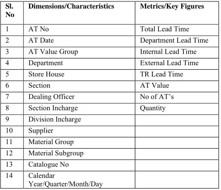
Below is the list of Dimensions, Attributes and Key Figures identified for Leadtime analysis. For characteristic attributes only those directly affecting Leadtime are considered.

Table 1: Characterstics, Key Figures

Sl. No

Dimensions/Characteristics Metrics/Key Figures

1 AT No Total Lead Time

2 AT Date Department Lead Time

3 AT Value Group Internal Lead Time 4 Department External Lead Time

5 Store House TR Lead Time

6 Section AT Value

7 Dealing Officer No of AT’s 8 Section Incharge Quantity 9 Division Incharge

10 Supplier 11 Material Group 12 Material Subgroup 13 Catalogue No 14 Calendar

Table 2: Attributes of each Dimension/Characteristic (Obtained from Master Data) Sl. No Dimension s/Characte rstics Attributes Remarks 1 AT (Acceptanc e to Tender)

1. AT No 2. AT Date 3. AT Value 4. Indent-Regn Date 5. TR Sent Date 6. TR Received Date 7. Currency Code 8. Currency Code Conv.

Relevant part of AT Master Table data

2 Department 1. Department Name 2. Department Code 3. Store House Code 4. Section Code 5. Material Type 6. Authorize-Direct-Indent Department/Sec tion Data 3 Dealing Officer

1. Dealing officer Name 2. Dealing officer Code 3. Active-Status

4. Controlling officer Code

5. DGM Group

Dealing officer/Section Incharge details

4 Supplier 1. Supplier Name 2. Supplier Code 3. Supplier

Category(10/11/06) 4. State/city

Relevant part of Supplier Master Data

5 Material Group

1. Mat Group 2. Mat Subgroup 3. Catalog No

4. Material Type(E/M/O) 5. Unit Codes(Fraction

Indicator)

Relevant part of Material Master Data 6 Calendar Year 1. Year 2. Quarter 3. Month 4. Day Time Dimension for each of above attributes

With above information, we can draw Logical data Model (LDM), which is a Table with relationship details between Characteristics & Key Figures. In LDM, Business Subjects that belong together are grouped around KF’s.

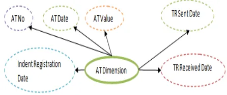
Figure 1: ERM diagram for Leadtime Analysis

In the above ERM, AT Dimension doesn’t have a specified hierarchy like Vendor, Department, Division Incharge, but should be modeled with attributes from master data as shown below.

Figure 2: Bubble Model for Attributes of AT Dimension The above LDM & Bubble Models are converted into ‘Extended Star Schema’ based on relationship between Entities as – Dimensions, Characteristics of dimension and attributes [3]. The Key Figures are further classified as – Basic Key Figures & Calculated Key figures for ‘Table Model’ drawn as below for the above dimensions. Table Model is very popular in Modeling functional requirements and representing data granularity. ‘X’ in the box indicates relevance of each data element. The legends for Key Figures (KF) in Table Model are given in Table 4 below.

Table 3: Table Model for ERM Diagram at Figure 1

KF Basic KF Calculated KF Granularity Time A T Department Dealing Officer Vendor Material Group Time

1 x Day x X X X X

2 x Day X X X X X X

3 x Day X X X X X

4 X Day X X X X X

5 x Day X X X X X

6 x Day X X X X X

7 x Day X X X X X X

8 x Day X X X X X x

Table 4: Key Figures Representation

Key Figure (KF) Meaning of Key Figure

1 Internal Leadtime

2 External Leadtime

3 Total Leadtime

4 Department Leadtime

5 TR Leadtime

6 Average Leadtime

7 AT Value (Price)

8 No of AT’s

9 Material Quantity

A. Enterprise Data warehouse Server and Data Modeling:

In enterprise system architecture, Data generated in the transactional system is brought over to Data warehouse server through customized data extractors. For our work, SAP BI server is used to create data elements for analysis. BI server runs on HP-UX Operating System (ia64 Machine Type) with Database System Oracle 11.2 and SAP Netweaver 7.0 as middleware.

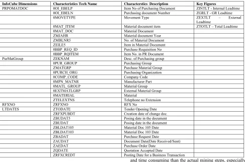
Table 5: Data Model for InfoCube Dimensions, Characteristics and Key Figures

InfoCube Dimensions Characteristics Tech Name Characterstics Description Key Figures

PRPOMATDOC 0OI_EBELP Item No of Purchasing Document ZINTLT - Internal Leadtime 0OI_EBELN Purchasing document Number ZGRLT - GR Leadtime

0MOVETYPE Movement Type ZEXTLT – External

Leadtime

0MAT_ITEM Material document item ZTOTLT – Total Leadtime

0MAT_DOC Material Document

ZMJAHR Material document Year

ZMBLNR5 No. of Material Document

ZEILE5 Item in Material Document

0BBP_REQ_ID Purchase Requisition No

0BBP_RQITEM Item No. in PR Document

PurMatGroup ZEKNAM Desc. of Purchasing group

0PUR_GROUP Purchasing Group

ZMATGRP Purchase Material Group

0PURCH_ORG Purchasing Organization

0COMP_CODE Company Code

0MPN_MATNR Manufacturer Part

0MATL_GROUP Material Group

0EXTMATLGRP External Material Group

0MATERIAL Material

ZTELEXTNS Telephone no Extension

RFXNO ZRFXNO RFX No

LTDATES ZTODATE Tender Opening Date

ZRFXPUBDT Creation date of change doc.

ZBUDAT5 Posing date in the document

ZBUDAT Posing date in the document

ZBLDAT105 Material Doc 105 Date

ZBLDAT103 Material Doc 103 Date

ZBADAT Purchase Request Date

ZAUDAT Document Date(Date Received/Sent)

ZAEDAT Purchase Order Date

ZQDATE Quotation Accepted Date

ZRFXCREDT Posting Date for a Business Transaction

III. DATA MINING MODELS AND KDD

The area of Data Mining encompasses techniques facilitating the extraction of knowledge from large amounts of data. These techniques include topics such as pattern recognition, machine learning, statistics, database tools and on-line analytical processing (OLAP). Data mining is one part of a larger process referred to as Knowledge Discovery in Database (KDD). The KDD process is comprised of the following steps [3]:

a. Data Cleaning b. Data Integration c. Data Selection d. Data Transformation e. Data Mining f. Pattern Evaluation g. Knowledge Presentation

The term data mining often is used in discussions to describe the whole KDD process, when the data preparation steps leading up to data mining are typically more involved

and time consuming than the actual mining steps, especially when the data is drawn from heterogeneous data sources.

Figure 3: Data Mining Algorithms for Prediction

A. Data mining algorithms are further classified into – Supervised & Unsupervised methods.

a. In Supervised Methods, both input data & valid output data is available for training process. The Model should match both Input & output patterns as defined in model’s parameters. During the training phase for Predictive Models, algorithms try to determine what relationships exist in data to match the “Known” outcome. Using the rules established in the learning phase, they predict outcome for a new unknown set of data. Supervised learning requires known output data records. Examples for supervised Learning are – Classification Trees, Bayesian Network, Regression (Linear, Non-Linear)

b. Unsupervised Methods are informative methods and do not depend on output patterns to detect rules, correlations and associations. They can reveal quick information about data. Unsupervised learning does not need a target or known values. Data clustering denotes the process of grouping data into clusters or classes such that the data in each cluster share a high degree of similarity while being very dissimilar to data from other clusters. Homogenous groups can be clustered in a predictive way. Examples for unsupervised Learning are – Clustering, Association Rules, Frequent set Mining, Constraint based data mining.

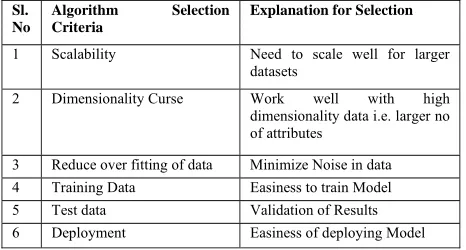
The selection criteria for choosing an appropriate Data Mining algorithm are given in Table 6.

Table 6: Selection Criteria for choosing Data Mining Algorithm

Sl. No

Algorithm Selection Criteria

Explanation for Selection

1 Scalability Need to scale well for larger datasets

2 Dimensionality Curse Work well with high dimensionality data i.e. larger no of attributes

3 Reduce over fitting of data Minimize Noise in data 4 Training Data Easiness to train Model 5 Test data Validation of Results 6 Deployment Easiness of deploying Model

IV. CLASSIFICATION ALGORITHMS

The classification method tries to categorize items to predefined target classes with the help of some algorithm. The building of classification model includes training data set with known, discrete target classes, which means that the classification results are always discrete. Classification targets vary from binary to multiclass attributes and the models try to predict which target class is correct with the help of descriptive relationships from the input attributes.

Data classification is a two phase process in which first step is the training phase where the classifier algorithm builds classifier with the training set of tuples and the second phase is classification phase where the model is used for classification and its performance is analyzed with the testing set of tuples [5]. Classification has numerous algorithms publicly available with varying application targets, from which some examples are Decision Tree, Bayesian networks, Support Vector Machines (SVM) and Rule Induction.

Decision Tree is a Classification scheme which generates a tree and a set of rules, representing the model of different classes, from a given data set. The set of records available for developing classification methods is generally divided into two disjoint subsets – Training set & Test set. The former is used for deriving the classifier, while the later is used to measure the accuracy of classifier. Also, the accuracy of the classifier is determined by the percentage of test examples that are correctly classified. Algorithmic framework for data mining models used in our analysis is discussed in next section.

A. Algorithmic Framework for Decision Trees: The goal is to find the optimal decision Tree by minimizing the generalization error along with number of nodes and average depth. Top–down decision trees algorithms are ID3 (Quinlan, 1986), C4.5 (Quinlan, 1993), CART (Breiman et al., 1984). Some consist of two conceptual phases: growing and pruning (C4.5 and CART). Other inducers perform only the growing phase [5]. Figure 4 shows a typical algorithm for Decision Tree using growing and pruning. In each iteration, the algorithm considers the partition of the training set using the outcome of a discrete function of the input attributes. The selection of the most appropriate function is made according to some splitting measures. After the selection of an appropriate split, each node further subdivides the training set into smaller subsets, until no split gains sufficient splitting measure or a stopping criteria is satisfied [6].

Tree Growing (S,A,y) Where:

S - Training Set A - Input Feature Set y - Target Feature

Create a new tree T with a single root node. IF One of the Stopping Criteria is fulfilled THEN Mark the root node in T as a leaf with the most common value of y in S as a label.

ELSE

IF best splitting metric > threshold THEN Label t with f(A)

FOR each outcome vi of f(A):

Set Subtreei = TreeGrowing (¾f(A)=viS,A,y). Connect the root node of tT to Subtreei with an edge that is labeled as vi

END FOR ELSE

Mark the root node in T as a leaf with the most common value of y in S as a label.

END IF END IF RETURN T

TreePruning (S,T,y) Where:

S - Training Set y - Target Feature T - The tree to be pruned DO

Select a node t in T such that pruning it Maximally improve some evaluation criteria IF t=Ø THEN T=pruned(T,t)

UNTIL t=Ø RETURN T

Figure 4: Top-Down Algorithm Framework for Decision Trees Given a training set S, the probability vector of the target attribute y is defined as:

|

| | , … ,

| |

| |

The goodness–of–split due to discrete attribute is defined as reduction in impurity of the target attribute after partitioning S according to the values , :

∆Φ ′

| _, | | |

| |

.Ø _,

a. InformationGain:

Information gain is an impurity-based criterion that uses the entropy measure as the impurity measure (Quinlan, 1987). , , , | | , . , _, Where: , | |

| | . log

| | | |

b. Gini Index:

Gini index is an impurity-based criterion that measures the divergences between the probability distributions of the target attribute’s values. The Gini index has been used in various works such as (Breiman et al., 1984) and (Gelfand et al., 1991) and it is defined as:

, 1 | _{| |} |

The evaluation criteria for selecting the attribute is defined as:

, ,

| _, |

| | . , , ,

B. Algorithmic Framework for Association Rule Mining (ARM):

Association rule mining (ARM) is an important core data mining technique to discover patterns/rules among items in a large database of variable-length transactions. The goal of ARM is to identify groups of items that most often occur together. Most of the research focuses on the frequent itemset mining subproblem, i.e., finding all frequent itemsets each occurring at more than a minimum frequency (minsup) among all transactions [6]. Well-known sequential algorithms include Apriori [7], Eclat [8], FP-growth [9], and D-CLUB [10].

Formal definition of Association Rule:

Let I , , … , be a set of literals, called items. Let D be a set of transactions, where each transaction T is a

set of items such that T I

A transaction T contains X, a set of some items in I, if X T

An association rule is an implication of the form X Y , where I,Y I , and X Y Ø

holds in the transaction set D with confidence c if c% of transactions in D that contain X also contain Y.

has support s in the transaction set D if s% of transactions in D contain X Y

Algorithm Apriori (Candidate Generation, Pruning) Initialize: k 1, = all the 1-itemsets;

Read the database to the support of to determineL .

L 1 ;

K 2; // k represents the pass number// While do

Begin

C gen_candiadte_itemsets with the given L Prune

For all transactions t T do

Increment the count of all candidates in C that are contained in t;

L C with minimum support; K k +1;

End Answer

The idea behind the a priori candidate generation procedure is that if an itemset X has minimum support, so do all subsets of X.

The Candidate – generation method is given below: C

For all itemsets do For all itemsets do

If 1 1 2 2 … 1

1

The pruning step eliminates the extensions of (k-1) itemsets which are not found to be frequent, from being considered for counting support.

Prune For all C

For all (k-1) subsets d of c do If d

Then C C \

C. Algorithmic Framework for Regression:

A Regression model predicts the value of a numerical data field, this is the target field, in a given data record from the known values of other data fields of the same record. The known values of other data fields are called input data fields or explanatory data fields. They can be numerical or categorical. The predicted value might not be identical to any value contained in the data used to build the model. A regression model is created and trained based on known data sets of data records whose target field values are known. You can apply the trained model to known or to unknown data. In unknown data, the values of the input fields are known, however, the value of the target field is not known [11]. A simple case of linear regression, where the sum of squared errors is minimized when–

∑

The maximum likelihood model is , which is used for prediction.

In Non-Regression Analysis, the Smoothing factor twists the line around the outliers for a better fit than the straight line. The Regression methods must be trained on historical data where the value to be predicted (on another set of data) is already known. During training, the function that defines the ‘best fit of line ‘through the data is generated. With the model trained, a new set of data can be executed and a predicted score generated [12].

V. IMPLEMENTATION STEPS

Since the value of each category of Leadtime needs to be predicted based on input data, we have focused on Predictive Models and accordingly supervised learning methods are chosen to predict outcome for a new unknown set of data [13]. Association Rule Mining (ARM) is also run on leading attributes of Leadtime to find support and confidence for group of items that occur most often together.

The Data Mining Models for Leadtime Analysis are designed and implemented in APD of SAP BI server. The

various steps associated with Model creation, ETL (Extract-Transform-Load) & data governance issues are outlined here [14]:

Step 1. Checked for data inconsistencies, if any, in the source data. We observed that data was found missing against many PR No’s for Characterstics like Material document no, Purchasing Group, RFx No etc. The same is discussed with business team and appropriate values are entered.

Step 2. Loaded data from source system to target InfoCube with appropriate ETL work as shown in Figure 5. Many fields required Transformations from source structure, for which coding is done in ABAP programming language in BI workbench. This appears as Routines and Formulae in Transformation Map. Also required Calculated Key figures are developed during ETL load to target.

Step 3. The infocube created in previous step is the source for training data mining model. APD workbench is used to design Data Mining Models for training, testing and generating error matrix on data.

Step 4: Decision Tree Model created. Here the model is trained and checked for accuracy and then model’s prediction is used on unknown data. Decision Tree offers 3 outputs – Predicted value, Predicted by Node, Predicted Probability. Both predicted value and probability can be specified up to 3 ranks.

Step 5: Regression Model created, trained & predictive scores are checked against known data. Model predictions are applied to unknown data. With each algorithm, Prediction accuracy, Training Error are observed. The data sets are divided into Training & Testing sets. Same no of records are used for both algorithms, to minimizing the sample bias. New Characteristics are added to check accuracy and representativeness of input sample.

Step 6: Association Rule Model is developed and checked for large framesets with required support and confidence. These frequent itemsets are further explored to find patterns in leading attributes.

VI. RESULTS AND DISCUSSION

The leading attributes which have a greater influence on Leadtime are identified as – Material Group, Purchase Group, Purchase Material Group, External Material Group and Dealing officer based on priority using the ranking algorithm available within APD. The results of Decision Tree, Regression and Association Rule Algorithms for different categories of Leadtime are compared.

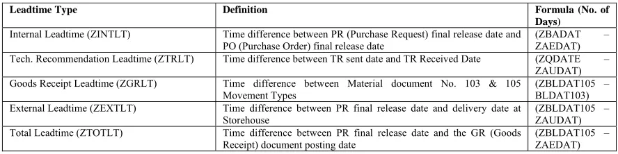
Table 7: Definition of Leadtime Types Predicted for Material Procurement (See Figure 5 for details)

Leadtime Type Definition Formula (No. of

Days)

Internal Leadtime (ZINTLT) Time difference between PR (Purchase Request) final release date and PO (Purchase Order) final release date

(ZBADAT – ZAEDAT)

Tech. Recommendation Leadtime (ZTRLT) Time difference between TR sent date and TR Received Date (ZQDATE – ZAUDAT) Goods Receipt Leadtime (ZGRLT) Time difference between Material document No. 103 & 105

Movement Types

(ZBLDAT105 – BLDAT103) External Leadtime (ZEXTLT) Time difference between PR final release date and delivery date at

Storehouse

(ZBLDAT105 – ZAUDAT) Total Leadtime (ZTOTLT) Time difference between PR final release date and the GR (Goods

Receipt) document posting date

Figure 5: Leadtime ETL Map with ABAP Routines & Formulae for Key Figures (SAP BIW) Table 8: Most frequent values in leading Characterstic Attributes

External Material Group

Material Group Purchasing Group Purchase Material Group

Dealing Officer

No of Records in % No of Records in % No of Records in % No of Records in % No of Records in %

21.14 27.19 29.91 0.51 28.79

9.15 12.24 12.24 0.51 26.26

9.02 11.37 9.77 0.51 16.16

6.67 8.90 7.05 0.51 10.61

5.19 5.56 6.67 0.51 5.56

4.45 5.19 6.30 0.51 4.55

3.71 4.33 4.33 0.51 3.54

3.09 3.71 4.08 0.51 2.53

2.97 2.97 2.97 0.51 2.02

2.97 1.85 2.22 0.51 6.34

Table 9: Frequency of values on Leadtime Metrics

Internal Leadtime External Leadtime GR Leadtime Total Leadtime Interval No of Records

in %

Interval No of Records in %

Interval No of Records in %

Interval No of Records in %

< 0 0.00 < 46 0.00 < 24 0.00 < 51 0.00

0 − < 1.2 0.12 46 − < 48.5 5.07 24 − < 26.1 11.87 51 − < 53.9 2.35

1.2 − < 2.4 0.49 48.5 − < 51 9.15 26.1 − < 28.2 10.01 53.9 − < 56.8 11.87

2.4 − < 3.6 0.12 51 − < 53.5 8.16 28.2 − < 30.3 7.79 56.8 − < 59.7 8.16

3.6 − < 4.8 0.62 53.5 − < 56 6.55 30.3 − < 32.4 3.96 59.7 − < 62.6 15.57

4.8 − < 6 4.94 56 − < 58.5 13.35 32.4 − < 34.5 3.96 62.6 − < 65.5 7.29

6 − < 7.2 73.92 58.5 − < 61 11.74 34.5 − < 36.6 3.83 65.5 − < 68.4 23.49

7.2 − < 8.4 3.71 61 − < 63.5 22.37 36.6 − < 38.7 14.71 68.4 − < 71.3 11.50

8.4 − < 9.6 16.07 63.5 − < 66 4.82 38.7 − < 40.8 25.09 71.3 − < 74.2 2.97

9.6 − < 10.8 0.00 66 − < 68.5 9.02 40.8 − < 42.9 9.02 74.2 − < 77.1 7.05 10.8 − < 12 0.00 68.5 − < 71 7.54 42.9 − < 45 7.54 77.1 − < 80 7.54

≥ 12 0.00 ≥ 71 2.22 ≥ 45 2.22 ≥ 80 2.22

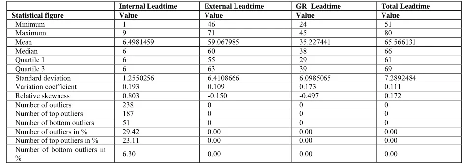
Outliers in input data used for training are not much significant, except for Total Leadtime (up to 20%) as shown in Table 10. The Model generation is an iterative process with an objective to achieve required accuracy after a specified number of trails [15]. It is observed that the

selection of characteristics, attributes has a major role in achieving desired accuracy and avoiding over fitting of trained data. The Accuracy of Decision tree and Regression Training Models is presented in Tables 11-12

Table 10: Statistical data on Leadtime Metrics used for Training Data Mining Models

Internal Leadtime External Leadtime GR Leadtime Total Leadtime

Statistical figure Value Value Value Value

Minimum 1 46 24 51

Maximum 9 71 45 80

Mean 6.4981459 59.067985 35.227441 65.566131

Median 6 60 38 66

Quartile 1 6 55 29 61

Quartile 3 6 63 39 69

Standard deviation 1.2550256 6.4108666 6.0985065 7.2892484

Variation coefficient 0.193 0.109 0.173 0.111

Relative skewness 0.803 -0.150 -0.497 0.172

Number of outliers 238 0 0 0

Number of top outliers 187 0 0 0

Number of bottom outliers 51 0 0 0

Number of outliers in % 29.42 0.00 0.00 0.00

Number of top outliers in % 23.11 0.00 0.00 0.00

Number of bottom outliers in

% 6.30 0.00 0.00 0.00

Table 11. Predictive Accuracy of Decision Tree Training Models

Model Type Leadtime Category Accuracy (%)

No of Trails

Pruning

Decision Tree Internal Leadtime 97.596 2 Yes Decision Tree External Leadtime 96.389 2 Yes Decision Tree GR Leadtime 95.754 2 Yes Decision Tree Total Leadtime 95.276 2 Yes

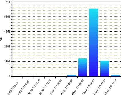
Percentage distribution of Leadtime values in Input Data generated by Linear Regression Model upon training is given in figures 6-9. Horizontal Axis represents No of days

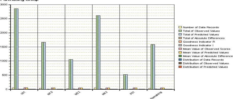
(intervals) for each category of Leadtime in input training data. Also data series for some leading attributes is given in figures 10-11.

Table 12: Predictive Accuracy of Regression Training Models

Model Type Leadtime Category Prediction Accuracy

Regression Type

Figure 6: % distribution of Total Leadtime in Training Data generated by Linear Regression

Figure 7: % distribution of External Leadtime in Training Data generated by Linear Regression

Figure 8: Percentage distribution of Internal Leadtime in Training Data generated by Linear Regression

Figure 9: Percentage distribution of GR Leadtime in Training Data generated by Linear Regression

Figure 11: Statistics on Purchasing Group Attribute in training data generated by Regression

Prediction Accuracy of Test Data for Decision tree is given in Tables 13 – 15. It is observed that accuracy of Decision Tree is reduced when some attributes are dropped to avoid over fitting of data. The model is subsequently deployed to predict unknown data. The initial sampling size for Decision Tree Model is kept as 15% with a Maximum value of 75%. The stopping condition of Model is - Min.

Leaf Cases -10, Min. Leaf Node accuracy – 95%. This is the point at which node will not split further. Node accuracy is calculated as –

NodeAccuracy

TotalNo.ofcasesatthenode – No.ofcaseswithmajorityclass TotalNo.ofcasesatthenode 100

Table 13: Node Accuracy of Decision Tree Model for Test data of Leadtime with leading attributes

Model Type Leadtime Category Accuracy (%) No of Trails No of Misclassifications Pruning

Decision Tree Internal Leadtime 99.670 2 2 Yes

Decision Tree External Leadtime 96.389 2 15 Yes

Decision Tree GR Leadtime 95.754 2 0 Yes

Decision Tree Total Leadtime 95.276 2 23 Yes

The Rule set generated by APD has given following results

with probabilities against each category of predicted value. Figures 12-15 show prediction graphs with more no of dimensional attributes.

Table 14: Rule Sets generated by Decision Tree Model with more attributes on Material Dimension

Figure 12: Total Leadtime Prediction graph w.r.t. Actual Values

Total Leadtime Internal Leadtime External Leadtime GR Leadtime

Predicted value Probability Predicted value Probability Predicted value

Probability Predicted value Probability

51 0.53 3 0.47 46 1.0 24 1.0

54 1.0 4 0.52 48 1.0 26 1.0

56 0.9 5 0.76 50 0.90 27 0.75

57 0.75 6 1.0 51 0.75 28 1.0

58 1.0 7 0.39 52 1.0 29 1.0

Figure 13: Internal Leadtime prediction Graph w.r.t Actual Values

Figure 14:External Leadtime prediction Graph w.r.t. Actual Values

Figure 15: GR Leadtime prediction Graph w.r.t Actual

A. Prediction Results of Decision Tree Model: For all categories of Leadtime predicted values are lesser than actual values, especially when more attributes are added. Also when outliers are present in leading attributes the predicted values deviated further from actual values.

B. Prediction accuracy using linear regression Model is above 95% for all categories of Leadtime which is shown graphically below. For Linear Regression Models, Regression is run for each value of discrete fields on the values tab (most frequent values are considered). Outliers are treated as separate instance. In Non-Linear Regression Models, the value of

Figure 16: % distribution of Total Leadtime Test Data generated by Linear Regression

Figure 17: % distribution of GR Leadtime Test Data generated by Linear Regression

Figure 18: % distribution of External Leadtime Test Data generated by Linear Regression

Figure 19: % distribution of Internal Leadtime Test Data generated by Linear Regression

Figure 20: Total Leadtime predicted vs. actual values (ZTOTLT is actual & sc_score002 is predicted)

Figure 22: Internal Leadtime predicted vs. actual values (ZINTLT is actual & sc_score001 is predicted)

Figure 23: GR Leadtime predicted vs. actual values (ZGRLT is actual & sc_score002 is predicted) For Association rule mining (ARM) model, only leading

attributes are considered as having more no of attributes is not producing any Association Rules with desired support and Confidence [16]. ARM Model could generate only 6-8 large Itemsets with support of 70 and confidence above 90,

with chosen attributes. We have further lowered support & confidence values to garner more association rules from main Characterstics [17]. The results are given in tables 15. Last 2 fields indicate results for large Item sets.

Table 15: ARM Model (Leading & Depending Items only)

Support Confidence Lift Leading Depth (No of Leading Items) Dependent Depth (No of depending items)

Support Cardinality

12 90 35 5 5 5.41 1

15 80 35 7 7 54.05 1

18 85 25 4 7 2.70 1

23 70 25 5 5 5.41 1

25 70 25 5 5 10.81 1

VII. CONCLUSIONS

The suitability of different algorithms will be known only on testing them empirically with different datasets and domain knowledge helps in choosing the right one. The results produced by Decision Tree have high degree of prediction accuracy when main attributes in Leadtime test data are considered for modeling. As more dimensional attributes like material movement type, RFx creation and purchasing details are added to simulate unknown data, the predictive accuracy drifted below expected value. Linear Regression model scaled better when more dimensional attributes are added as seen from predicted vs. actual value graphs.

The results also showed that continuous attribute prediction with regression suffered if there were no approximately linear or Gaussian distributions with enough predictive independent attributes. Categorical attributes needed to have a limited number of values to make it

possible to use them in classification as predictors and the lack of descriptive attributes implied problems with the attribute selection or collected source attributes in Leadtime data. ARM results indicate that Leadtime data is not suited for mining frequent itemsets with desired support and confidence. This is not giving any definite relationship from AR formulations & hence ARM results are ignored for analysis. From our study, it is clear that Classification & Regression Models of data mining would give better results for analyzing material procurement Leadtime data, with an objective to predict the class of records whose class label is not known. The criterion for scalability was fulfilled to the extent of available test material and the built-in functionality criterion was completely fulfilled.

VIII. REFERENCES

[2] J Miller, Jiawei Han., Chapman & Hall.,Geographic Data Mining and Knowledge Discovery by Harvey, CRC Press [3] Jiawei Han and Micheline Kamber (2006), Data Mining

Concepts and Techniques, published by Morgan Kauffman, 2nd _Edition

[4] Closed loop BI -

http://www.microstrategy.com/software/business-intelligence/closed-loop-bi/

[5] M. Tim Jones .,Artificial Intelligence, A systems Approach , Computer Science Series

[6] Lior Rokach, Oded Maimon, Decision Trees, Department of Industrial Engineering, Tel-Aviv University

[7] R. Agrawal, T. Imielinski, and A. Swami. Mining Association Rules between Sets of Items in Large Databases. In Proceedings of the 1993 International Conference on Management of Data (SIGMOD 93), ACM Press., pages 207-216, May 1993

[8] R. Agrawal, R. Srikant. Fast Algorithms for Mining Association Rules (1994) Proc. 20th Int. Conf. Very Large Data Bases, VLDB

[9] Mohammed J. Zaki, Srinivasan Parthasarathy, Mitsunori Ogihara, and Wei Li. New algorithms for fast discovery of association rules.

[10] Jianwei Li, Alok Choudhary, Nan Jiang, and Wei-keng Liao. Mining frequent patterns by differential refinement of clustered bitmaps. In Proc. of the SIAMInt’l Conf. on Data Mining, April 2006.

[11] Padhraic Smyth,,University of California, ‘Lecture Notes on Data Mining Regression Algorithms’

[12] Dr. Gary Parker, vol 7, 2004, Data Mining: Modules in emerging fields

[13] Kurt Thearling, Lecture Notes on Data Mining Modeling, accessed at www.thearling.com

[14] Galit Shmueli., Nitin R. Patel., Peter C. Bruce., Data Mining for Business Intelligence, October 26, 2010, John Wiley & Sons Inc New Jersey., PP 110-125.

[15] Michael J Berry., Gordon S Linoff., Mastering Data Mining, Published by John Wiley & Sons, Inc, pp 183-195 [16] Pang-Ning Tan, Michael Steinbach, Vipin Kumar,

Introduction to Data Mining, March 2006., Addision-Wesley.,Chapter 6 Association Analysis PP 330-340 [17] Hand, D.et al., 2001., Principles of Data Mining.,