Segmentation Through Lbp Based Defocus Blur

(1)

Available online: https://edupediapublications.org/journals/index.php/IJR/ P a g e | 2233

Segmentation through Lbp Based Defocus Blur

V.Sai Padmini & K.Chaitanya Lakshmi

1 _{PG Scholar, Dept. of ECE,}_{AKRG College of Engineering, Nalajerla,}_{W.G Dist, AP, India.} 2 _{Asst. Professor, Dept. of ECE,}_{AKRG College of Engineering, Nalajerla,}_{W.G Dist, AP, India.}

Abstract:

When an image is captured by any optical imaging devices in that image, defocus blurs is the common undesirable issue. So defocus blur is extremely common in images captured using optical imaging systems. The presence of the blur is one of the major drawbacks which occur frequently in the processing of the digital images in the real time scenario. We proposed sharpness metric in this paper based on Local Binary Patterns (LBP) and a robust segmentation algorithm for the defocus blur. The proposed sharpness metric exploits the observation that the majority local image patches in blurred regions have considerably fewer of bounds native binary patterns compared with those in sharp regions. Tests on hundreds of partially blurred images were used to evaluate our blur segmentation algorithm and comparator methods. The results shows that our algorithm achieves comparative segmentation results with have big speed advantage over the others.

Keywords: Digital image processing, LBP pattern, Sharpness, Segmentation, Defocus Blur method.

1. I

NTRODUCTION

Defocus is the phenomenon in which image is out of focus and it reduces the sharpness and contrast of image. Signal processing is a field in electrical engineering and in mathematics that deals with examine and processing of signals that is analog and digital signal and also deals with operations like storing operation filtering operations on signals. These signals involves transmission, sound or voice , image signals .From these the field that deals with the type of signals in which the input is taken as image and the output is also an image is done is image processing. As it suggests, it works with the processing on images. Image processing in which images are to be analyzed and acted upon by peoples. It can be further divided into analog image processing and digital image processing.

(2)

Methods that explicitly model spatially variant blur typically restore small image patches within which blur can be treated as invariant, and restored patches are stitched together. Efficient and accurate detection

of blurred or non-blurred regions is useful in several contexts including: 1) in avoiding expensive post-processing of non-blurred regions (e.g. deconvolution); 2) in computational photography to identify a blurred background and further blur it to achieve the artistic bokeh effect, particularly for high-depth-of-field cellular phone cameras; and 3) for object recognition in domains where objects of interest are not all-in-focus (e.g. microscopy images) and portions of the object which are blurred must be identified to ensure proper extraction of image features, or, if only the background is blurred, to serve as an additional cue to locate the foreground object and perform object-centric spatial pooling [40]. The purpose of segmentation of defocus blur is to separate blurred and non-blurred regions so that any aforementioned post-processing can be facilitated. Herein, this problem is explicitly addressed without quantifying the extent of blurriness and a new sharpness metric based on Local Binary Patterns (LBP)and LLBP is introduced.

2. LITERATURE

REVIEW

Fergus et al. [1] proposed a method that Camera shakes during exposure May causes to objectionable image blur and damage photographs. Conventional blind deconvolution techniques rarely assume frequency-domain parameters on images for the motion path while camera shake. Real camera motions can follow up the convoluted way and spatial domain prior can better retains visually image properties. They introduced a method to remove the effects of camera shake from blurred images. This method assumes that a uniform camera blur over the image and also negligible in-plane camera rotation. In order to calculate the blur from the camera shake, the person must specify an image region without saturation effects. They showed results for a wide

variety of digital photographs which are taken from personal photo collections.

Bae and Durand[2] presented the image processing technique in which defocus magnification is used to perform blur estimation. To maximize defocus blur caused by lens aperture by taking a single image then estimate the size of blur kernel at edges and further they spread this technique to the whole image. In this approach multi scale edge detector is used and model fitting that obtain the size of bur propagate the blur measure by assuming that blurriness is smooth where

intensity and color are approximately similar. Using defocus map, they enhance the existing blurriness, which means that blur the blurry regions and keeps the sharp regions sharp. In comparison to other methods more difficult issues arises such as depth from defocus, so this proposed method do not need precise depth estimation and do not need to disambiguate texture less regions. The method models changes in energy at all frequencies with blur and not just very high frequencies (edges).

(3)

demonstrated that they can produce images that are more uniformly sharp then those images which produced with spatially-invariant deblurring technique.

Tai and brown in [5] As Image defocus estimation is useful for several applications including deblurring, blur enlargement, measuring image quality, and depth of field segmentation. They proposed a simple effective approach for estimating a defocus blur map based on the relationship of the contrast to the image gradient in a local image region and call this relationship the local contrast prior. The advantage of this approach is that it does not need filter banks or frequency decomposition of the input image; infact it only needs to compare local gradient profiles with the local contrast. They discuss the idea behind the local contrast prior and shown its results on a variety of

experiments. And it‟s found that for natural in-focus images, this distribution follows a similar pattern. They verified this distribution by plotting the distribution of the LC in images suffered from different type of degradation. This prior is useful in estimating defocus blur, in segmenting in focus regions from depth-of-field image and in ranking image quality.

Chakrabarti et al. [6] suggested a method for analyzing spatially changing blur. This method uses a sub-band decomposition to separate the “local frequency” components of an image, and an image model based on a Gaussian Scale Mixture to handle the variation in gradient statistics among local windows of a single image. These allow computing the particular window in an image being blurred by a candidate kernel, and this likelihood conveniently involves a preference for sharp edges without being badly affected by the natural variation in edge contrast that occurs in a typical image. Method proposed method used to determine the orientation and degree of motion in images with moving objects, and by combining them with color information, it shows that one can obtain reasonable segmentations of the objects also the proposed tools can be used to analyze motion blur, and this method is enough to handle any case of spatiallyvarying blur

.

Fig. 1: LLBP operator with line length 9 pixels, 8 bits considered

The motivation of Local Line Binary Pattern (LLBP) is from Local Binary Pattern (LBP) due to it summarizes the local spatial structure (micro-structure) of an image by thresholding the local window with binary weight and introduce the decimal number as a texture presentation. Moreover, it consumes less computational cost. The basic idea of LLBP is similar to the original LBP, but the difference are as follows: 1) its neighbourhood shape is a straight line with length N pixel, unlike in LBP which is a square shape. 2) the distribution of binary weight is started from the left and the right adjacent pixel of center pixel (20) to the end of left and right side.

The algorithm of LLBP, it first obtains the line binary code along with horizontal and vertical direction separately and its magnitude, which characterizes the change in image intensity such as edges and corners, is then computed.

4. P

ROPOSED

M

ETHOD

(4)

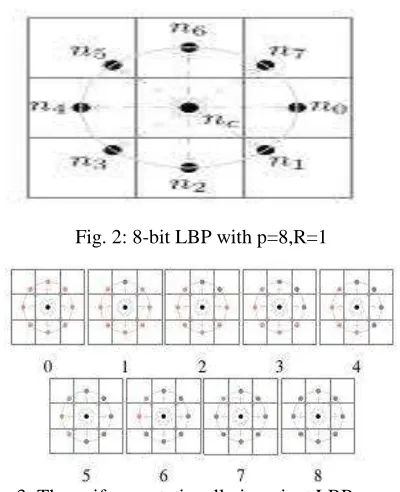
Fig. 2: 8-bit LBP with p=8,R=1

Fig. 3: The uniform rotationally invariant LBP.

corresponds to the intensities of the P

pixels located on a circle of radius R centered at , and TLBP>0 is a small, positive threshold in order to achieve robustness for flat image regions as in [19]. Figure 4 shows the locations of the neighboring pixels for P=8 and R=1. In general, the point’s do not fall in the center of image pixels, so the intensity of is obtained with bilinear interpolation. A rotation invariant version of LBP can be achieved by performing the circular bitwise right shift that minimizes the value of the LBP code when it is interpreted as a binary number.

In this way, number of unique patterns are reduced to 36. Ojala et al. found that not all rotation invariant patterns sustain rotation equally well [34], and so proposed using only uniform patterns which are a subset of the rotation invariant patterns. A pattern is uniform if the circular sequence of bits contains no more than two transitions from one to zero, or zero to one. The non-uniform patterns are then all treated as one single pattern. This further reduces the number of unique patterns to 10 (for 8-bit LBP), that is, 9 uniform patterns, and the category of non-uniform patterns. The uniform patterns are shown in Figure 5. In this figure, neighboring pixels are colored blue if their intensity difference from centre pixel is larger

than TLBP, and we say that it has been “triggered”, otherwise, the neighbours are colored red.

Our proposed sharpness metric exploits these observations:

Where

8-,bit

is the number of rotation invariant uniform LBP pattern of type i,and N is the total number of pixels in the selected local region which serves to normalize the metric so that ∈[0,1]. One of the advantages of measuring sharpness in the LBP domain is that LBP features are robust to monotonic illumination changes which occur frequently in natural images. The threshold TLBP in Equation (3.1) controls the proposed metric’s sensitivity to sharpness.

There is a sharp fall-off between σ =0.2 and σ=1.0 which makes the intersection of response value range of sharp and blur much smaller than the other metrics. When σ approaches 2, responses for all patches shrinks to zero which facilitates segmentation of blurred and sharp regions by simple thresholding. Moreover, almost smooth region elicit a much higher response than smooth region compared with the other metrics. Finally, the metric response is nearly

monotonic, decreasing with increasing blur, which should allow such regions to be distinguished with greater accuracy and consistency.

NEW BLURSEGMENTATIONALGORITHM

This section presents our algorithm for segmenting blurred/sharp regions with our LBP-based sharpness

metric it is summarized in Figure 12. The algorithm has four main steps: multi-scale sharpness map generation, alpha matting initialization, alpha map computation, and multi-scale sharpness inference.

(5)

In the first step, multi-scale sharpness maps are generated using . The sharpness metric is computed for a local patch about each image pixel. Sharpness maps are constructed at three scales where scale refers to local patch size. By using an integral image [50], sharpness maps may be computed in constant time per pixel for a fixed P and R.

B. Alpha Matting Initialization

Alpha matting is the process of decomposing an image into foreground and background. The image formation model can be expressed as

Where the alpha matte, α x,y, is the opacity value on pixel position(x,y). It can be interpreted as the confidence that a pixel is in the foreground. Typically, alpha matting requires a user to interactively mark known foreground and background pixels, initializing those pixels with α =1andα =0, respectively. Interpreting “foreground” as “sharp” and background as “blurred”, we initialized the alpha matting process automatically by applying a double threshold to the sharpness maps computed in the previous step to produce an initial value of α for each pixel.

Where s indexes the scale, that is, masks (x,y) is the initial α-map at the s-th scale.

C. Alpha Map Computation

The α-map was solved by minimizing the following cost function as proposed by Levin

( ) = + ( − ) ( − )(3.5)

Where α is the vectorized α-map, Is one of the vectorized initialization

alpha maps from

= ( , )

the previous step, and is the matting Laplacian matrix. The first term is the regulation term that ensures smoothness, and the second term is the data fitting term that encourages similarity to . For more

(6)

Available online: https://edupediapublications.org/journals/index.php/IJR/ P a g e | 2238 D. Multi-Scale Inference

After determining the alpha map at three different scales, a multi-scale graphical model was adopted to make the final decision . The total energy on the graphical model is expressed as

Whereℎ= is the alpha map for scale sat pixel location i that was computed in the previous step, and ℎ is the sharpness to be inferred. The first term on the right hand side is the unary term which is the cost of assigning sharpness value ℎ to pixel i in scale . The second is the pairwise term which enforces smoothness in the same scale and across different scales. The weight β regulates the relative importance of these two terms. Optimization of Equation 3.6 was performed using loopy belief propagation.

(7)

The main steps are shown on the left; the right shows each image generated and its role in the algorithm. The output of the algorithm is h 1.

5. S

IMULATION

R

ESULTS

Figure: 1Segmentation with LBP

Figure: 2 Segmentation with LLBP

6. C

ONCLUSION

We successfully proposed easy and effective sharpness metric for the segmentation of partially blurred image into blurred and non blurred regions. This metric is mostly based on the distribution of uniform LBP patterns in blurred and non blurred regions. The direct use of some sharpness measure based on the sparse representation gives the comparative results to our proposed method. By integration the metric into a multiscale information propagation frame work, it is able compare results with the progressively as well as with state of art. We’ve shown that the algorithm’s performance is maintained once victimization an mechanically associated adaptively taken threshold Tseg. Our sharpness metric measures the amount of sure LBP

(8)

REFERENCES

[1] R. Achanta, S. Hemami, F. Estrada, and S. Susstrunk, “Frequency-tuned salient region detection,” in Proc. IEEE Conf. Comput. Vis. Pattern Recognit. (CVPR), Jun. 2009, pp. 1597–1604.

[2] H.-M. Adorf, “Towards HST restoration with a space-variant PSF, cosmic rays and other missing data,” in Proc. Restoration HST Images Spectra-II, vol. 1. 1994, pp. 72–78.

[3] T. Ahonen, A. Hadid, and M. Pietikäinen, “Face description with local binary patterns: Application to face recognition,” IEEE Trans. Pattern Anal. Mach. Intell., vol. 28, no. 12, pp. 2037–2041, Dec. 2006.

[4] S. Bae and F. Durand, “Defocus magnification,” Comput. Graph. Forum, vol. 26, no. 3, pp. 571–579, 2007.

[5] K. Bahrami, A. C. Kot, and J. Fan, “A novel approach for partial blur detection and segmentation,” in Proc. IEEE Int. Conf. Multimedia Expo (ICME), Jul. 2013, pp. 1– 6. J. Bardsley, S. Jefferies, J. Nagy, and R. Plemmons, “A computational method for the restoration of images with an unknown, spatially-varying blur,” Opt. Exp., vol. 14, no. 5, pp. 1767– 1782, 2006.

[6] G. J. Burton and I. R. Moorhead, “Color and spatial structure in natural scenes,” Appl. Opt., vol. 26, no. 1, pp. 157–170, 1987. [7] A. Buades, B. Coll, and J.-M. Morel, “A