Boosted Jet Tagging with Jet-Images and Deep Neural Networks
Michael Kagan1,a, Luke de Oliveira2, Lester Mackey2, Benjamin Nachman1,2,b, and Ariel Schwartzman1,c
1SLAC National Accelerator Laboratory, Menlo Park, CA, USA 2Stanford University, Stanford, CA, USA
Abstract.Building on the jet-image based representation of high energy jets, we develop computer vision based techniques for jet tagging through the use of deep neural networks. Jet-images enabled the connection between jet substructure and tagging with the fields of computer vision and image processing. We show how applying such techniques using deep neural networks can improve the performance to identify highly boosted W bosons with respect to state-of-the-art substructure methods. In addition, we explore new ways to extract and visualize the discriminating features of different classes of jets, adding a new capability to understand the physics within jets and to design more powerful jet tagging methods.
1 Introduction
Jets, or collimated streams of particles arising from the production of high energy quarks and gluons, are crucial signatures for discovering signs of new physics at the Large Hadron Collider (LHC) [1]. Quarks and gluons, and subsequently jets, are produced ubiquitously from the LHC proton-proton collisions. However, in many theories of new physics, new TeV-mass-scale particles decay into high energyW±,Z,Hbosons, and top quarks. These high energy bosons and top quarks can subsequently decay into single jets containing all of their decay products. Identifying, ortagging, the jets from bosons and top quarks is thus vital to reconstruct and identify signs of new TeV-mass-scale parti-cles. The field of jet-substructure (see [2–4] and references therein) has emerged to overcome this challenge, whereby physics inspired features are engineered to exploit the differences in the internal structure of jets produced by bosons and top quarks from that of jets produced directly from quarks and gluons. Concurrently, modern computer vision and machine learning techniques have made great progress in recent years in deep learning [5–7]; large multi-hidden layer neural networks operating on low level information (e.g. pixels in an image), without feature engineering, have been found to learn complex representations of information within images and efficiently use this information for classification.
The jet-images approach to jet tagging combines computer vision with jet-substructure. Jet mea-surements from LHC detectors are formatted into images, where detector energy meamea-surements play
ae-mail: [email protected]
be-mail: [email protected]
the role of pixel intensities, and the jet-images are analyzed using computer vision inspired tech-niques. The computer vision techniques include linear methods, such as Fisher discriminant analysis, and deep learning methods, including convolutional and dense MaxOut neural network architectures. These techniques not only provide improved discrimination power, but also insight into the physics learned for discrimination.
The power of the images and computer vision techniques is explored in a benchmark jet-substructure problem, discriminating high energyW±bosons from quarks and gluons, as discussed in references [8] and [9]. We refer the reader to these references for further details.
2 Samples and selection
To study the jet-images technique, the benchmark task of discriminating high energyW± bosons from quarks and gluons is examined. Monte Carlo (MC) simulations of proton-proton collisions at
√
s=14 TeV based on the Pythia8.170 [10,11] event generator are used. High energyW±bosons are simulated through the decay of a hypothetical new heavyWboson which decays to oneW±boson and oneZboson. Subsequently, theWis forced to decay hadronically (W →qq), and theZto decay invisibly (Z→νν). The background is the generic (multijet) production of quarks and gluons.
Since the classification performance can depend on the transverse momentum,pT, and jet mass,
m, of the jets, we focus our studies on a restricted range of 250 GeV/c< pT < 300 GeV/c, and a
65 GeV/c2< m<95 GeV/c2mass window that contains the peak of theW. The minimum angular
spread of theWdecay products is approximatelyΔR= Δη2+ Δφ2≈0.6, whereΔηandΔφare the
distances betweenWboson decay products in (η, φ) coordinates. Further, to remove any dependence on the jet transverse momentum, we re-weight the signal to have the same pT distribution as the
background.
The discrete size and finite acceptance of a real detector are modeled by binning the particles into cells with size 0.1×0.1 in (η, φ) extending out to η = 5.0. Each cell’s 4-vector is defined bypj = iincident onjEi(cosφj/coshηj,sinφj/coshηj,sinhηj/coshηj,1), where the sum runs over
particles indent on the cell.
Jets are built by clustering the cells using the anti-ktalgorithm [12] with distance parameterR=
1.0, via FastJet[13] 3.0.3. The large distance parameter is used in order to capture all the decay products of a boostedW boson. To reduce the impact of pileup1 and underlying event, jets are are
trimmed [14] by re-clustering the constituents intoR=0.3ktsubjets and dropping those which have psubjet
T <0.05×p jet T.
In order to compare the jet-images approach with standard substructure techniques, we compare performance with known highly performant jet substructure features. These features are thejet mass defined asm2jet =i,jpipjwith jet constituent four-vectorspi,n-subjettiness[15] in the form ofτ21
using the winner-take-all axis definition [16], and the distance in (η, φ) space between subjets of the trimmed jet (ΔR).
3 Jet-images and pre-processing
Jet-images are formed by taking a 25×25 cell grid around the jet axis, with the intensity of jet-image pixelidefined to be the corresponding cell transverse energypT,i=Ei/cosh(ηi).
In order for machine learning algorithms to learn more efficiently, we make use of space-time symmetries to pre-process the jet-images into a standardized representation. The pre-processing steps are:
• Translation: Jet-images are translated such that the leadingpTsubjet is located at (η, φ) =(0,0).
Note that translations inφare effectively rotations around the detectorz-axis, while translations in
ηare Lorentz boosts along thez-axis. As such, translations inηcan alter the mass of a jet-image if the pixel energies are kept fixed. However, the transverse energy is invariant to suchηtranslations, and thus is used for the pixel intensities.
• Rotation: Jets are rotated such that the second leadingpTsubjet is aligned along the vertical axis of
the jet-image. If the jet has only one subjet, the first principle component of the energy distribution in (η, φ) is rotated to align with the vertical axis of the jet-image.
• Parity Flip: After rotation, images are flipped over the vertical axis such that the right side of the
image has a higher energy than the left. This helps to standardize the location of additional radiation in the jet-image.
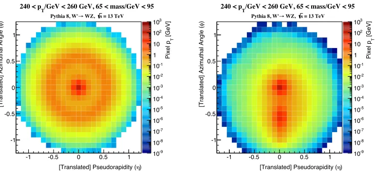
After pre-processing, the leading subjet within the jet-image is located at the center of the image, and the second subjet (if it exists) is aligned along the vertical axis of the image. In facial recognition tasks, this is equivalent to aligning the eyes within an image of a face. With such a standardized jet-image representation, the machine learning algorithms do not need to learn about the symmetries in the jet-image, thus allowing the learning to focus more effectively on discrimination. The effect of the pre-processing on a collection ofWjets can be found in Figure1.
[GeV] T Pixel p -9 10 -8 10 -7 10 -6 10 -5 10 -4 10 -3 10 -2 10 -1 10 1 10 2 10 3 10 ) η
[Translated] Pseudorapidity (
-1 -0.5 0 0.5 1
)
φ
[Translated] Azimuthal Angle (
-1 -0.5 0 0.5 1
= 13 TeV s WZ,
→
Pythia 8, W'
/GeV < 260 GeV, 65 < mass/GeV < 95
T
240 < p
[GeV] T Pixel p -9 10 -8 10 -7 10 -6 10 -5 10 -4 10 -3 10 -2 10 -1 10 1 10 2 10 3 10 ) η
[Translated] Pseudorapidity (
-1 -0.5 0 0.5 1
)
φ
[Translated] Azimuthal Angle (
-1 -0.5 0 0.5 1
= 13 TeV s WZ,
→
Pythia 8, W'
/GeV < 260 GeV, 65 < mass/GeV < 95
T
240 < p
Figure 1. The average jet-image forWjets before (left) and after (right) pre-processing. The average is taken over jet-images with 240 GeV/c<pT<260 GeV/cand 65 GeV/c2<m<95 GeV/c2.
4 Deep learning architectures and training
state-of-the-art architectures: fully connected MaxOut networks [6], and convolutional neural net-works [5].
Complete descriptions of the architectures can be found in reference [9], and are only briefly de-scribed here. The MaxOut network consists of two MaxOut layers followed by two fully connected layers, followed by a classification layer. The convolutional network (ConvNet) consists of three con-volution layers, followed by one fully connected layer, followed by a classification layer. Concon-volution kernel sizes were 11×11 in the first convolutional layer, and 3 in subsequent convolutions. The atyp-ically large kernel size in the first convolution was found to help performance on the relatively sparse jet-images (only about 5–10% of pixels contain energy on average in a jet-image). Each convolution is followed by a max-pooling layer [17] and then by a dropout layer [7]. All MaxOut, dense, and con-volutional layers use the rectified linear unit (ReLU) activation function [18], while the classification layer uses sigmoid activations.
All deep learning experiments were conducted in Python with the Keras [19] deep learning library, utilizing NVIDIA C2070 graphics cards. 8 million examples were used for training, with an additional 2 million validation samples for tuning the hyper-parameters, and 3 million examples were used for testing. Signal examples were weighted such that the total sum of weights was the same as the total number of background examples. These weights were used by the cost function in the training and in the ROC curve computations of the test samples. The networks were trained with the Adam [20] algorithm. The training consisted of 100 epochs, with a 10 epoch patience parameter on the increase in area under the ROC curve between 0.2 and 0.8 on a validation set. Batch sizes of 32 were used for the MaxOut network, while batch sizes of 96 were used for the convolution networks.
5 Results
The primary figure of merit used in this note to compare the performance of different classifiers is the ROC curve, which shows the quark/gluon background rejection (the inverse misclassification efficiency) as a function of theW jet signal efficiency. Efficiencies and rejection are computed by scanning thresholds on the signal-to-background likelihood ratio distribution (i.e. the optimal use of the variables).
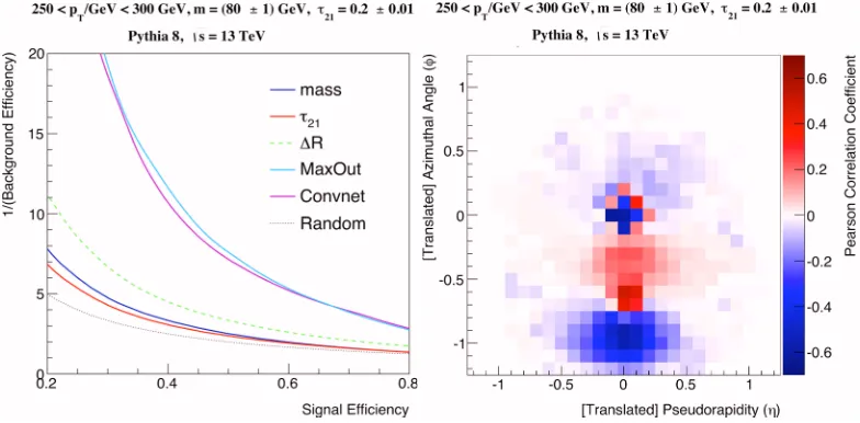
The ROC curve showing the DNNs as well as several substructure variables can be found on the left in Figure2. Both DNNs are seen to have significantly better rejection than the substructure variables for all efficiencies, with an improvement in rejection of about 2 at a signal efficiency of 30%. We also see that the MaxOut network tends to outperform the ConvNet, which we believe is due to difficulties for convolutional networks to learn rich discriminating information from kernels when images are sparse.
In order to understand if the DNNs have learned the information contained within the substructure variables, we combine the DNN outputs with substructure variables into a single discriminant using the likelihood ratio of the 2D distribution of the DNN and the substructure variable. The combination with the ConvNet is shown on the right in Figure2. We can see that the combination withΔRand
τ21adds little discrimination to the baseline performance of the ConvNet, indicating that the ConvNet
has learned the discriminating information contained in these variables. However, when the jet mass is combined with the ConvNet, the performance is seen to increase, indicating that the ConvNet has not completely learned the mass information. Similar behavior is found for the MaxOut network.
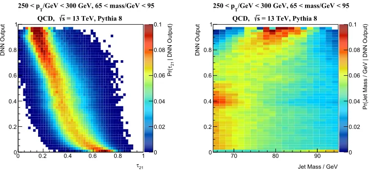
To examine more deeply into the information learned by the DNNs, Figure3shows the 2D dis-tribution ofτ21 (left) and jet mass (right) conditioned on the ConvNet output, i.e.p(X|DNN output)
whereXis the substructure variable. As we can see, the ConvNet output is strongly correlated with
Signal Efficiency
0.2 0.4 0.6 0.8
1/(Background Efficiency)
0 50 100 150
= 13 TeV, Pythia 8 s
/GeV < 300 GeV, 65 < mass/GeV < 95
T
250 < p
mass 21 τ R Δ Fisher MaxOut Convnet Convnet-norm Random Signal Efficiency
0.2 0.4 0.6 0.8
1/(Background Efficiency)
0 50 100 150
= 13 TeV, Pythia 8 s
/GeV < 300 GeV, 65 < mass/GeV < 95
T
250 < p
mass+Convnet +Convnet 21 τ R+Convnet Δ MaxOut Convnet Convnet-norm Random
Figure 2.ROC curves comparing DNNs with substructure discriminants (left), and ROC curves when DNNs are combined with substructure variables (right).
with mass is not as strong, with the distributions of mass significantly spread out over various Con-vNet output values. While some correlation is present, the network does not seem to have learned all information contained in the jet mass.
In order to study what is learned by the DNNs beyond known substructure variables, we examine the networks in several ways. First, we find the 500 most activating images for a given neuron,
| DNN Output)
21 τ Pr( 0 0.02 0.04 0.06 0.08 0.1 21 τ
0 0.2 0.4 0.6 0.8 1
DNN Output 0 0.2 0.4 0.6 0.8
1 QCD, s = 13 TeV, Pythia 8
/GeV < 300 GeV, 65 < mass/GeV < 95 T
250 < p
Pr(Jet Mass / GeV | DNN Output)
0 0.02 0.04 0.06 0.08 0.1
Jet Mass / GeV
70 80 90
DNN Output 0 0.2 0.4 0.6 0.8
1 QCD, s = 13 TeV, Pythia 8
/GeV < 300 GeV, 65 < mass/GeV < 95 T
250 < p
Figure 3. 2D distribution of τ21 (left) and jet mass (right) conditioned on the ConvNet output,
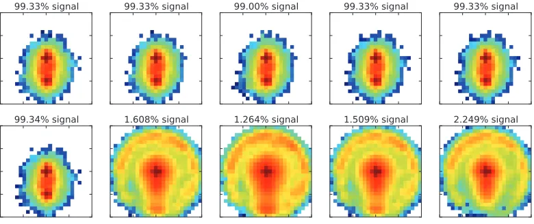
and visualize the average of these images. This is shown in Figure4for several neurons in the last hidden layer of the ConvNet. Also shown above each images is the fraction of images found to be most activating for each neuron that were signal images. As we can see, the signal correlated neurons have a clear two-prong structure with information between the leading two subjets but very little information outside of the two-prong structure. In contrast, background correlated neurons have much broader energy distributions indicating the presence of additional wide-angle radiation beyond the leading two subjets.
Figure 4.Average most activating input images for several neurons in the last hidden layer of the ConvNet.
To further understand how the DNNs use the information present in the jet-images for discrimi-nation, we compute the Pearson correlation coefficient for each jet-image pixel with the output of the DNN. These correlations with the ConvNet can then be visualized as an image, as seen in Figure5. From this correlation image, we see that the presence of a leading subjet at the center of the image provides little discrimination power. This is not surprising, as both signal and background jets have at least one high energy subjet. However, the location of the subleading subjet is strongly correlated with signal-like images, as seen by the red region at (η, φ)≈(−0.5,0). In addition, radiation present around the the leading subjet and radiation at the periphery of the image away from either subjet is correlated with background like images. This indicates that the radiation pattern beyond the leading subjets provides important information for discrimination.
Figure 5.Pearson correlation coefficient of each input pixel with the ConvNet output.
while radiation at the periphery is correlated with background like images. This could be due to the difference between radiation patterns of the decays of a color singletW boson, as apposed to the de-cays of a color octet gluon or color triplet quark. While features engineered to exploit such colorflow information have been studied in the past [21], the features learned here may present a new way to access this information for improved discrimination.
6 Conclusions
In this paper, we have used the paradigm of jet-images to interpret LHC data based on tools in-spired by image processing, computer vision, and deep learning. Deep learning proved to be powerful paradigm for jet tagging when combined with jet-images, significantly improving performance over state-of-the-art jet substructure features. The performance of deep learning techniques was aided by domain specific inputs, whereby physics inspired pre-processing allowed deep neural networks to learn powerful discriminating information without having to simultaneously learn the symmetries of space-time. Finally, we showed several techniques to extract information about what the deep neural networks are learning. A key aspect to this was being able to visualize the learned information in several ways.
Acknowledgments
This work was supported by the Stanford Data Science Initiative and by the US Department of Energy (DOE) grant DE-AC02-76SF00515.
References
[1] L. Evans, P. Bryant, JINST3, S08001 (2008)
[2] A. Altheimer et al., J. Phys.G39, 063001 (2012),arXiv:1201.0008 [3] A. Altheimer et al., Eur. Phys. J.C74, 2792 (2014),arXiv:1311.2708 [4] D. Adams et al., Eur. Phys. J.C75, 409 (2015),arXiv:1504.00679 [5] K. Simonyan, A. Zisserman (2014),arXiv:1409.1556
[6] I.J. Goodfellow, D. Warde-Farley, M. Mirza, A. Courville, Y. Bengio (2013), arXiv:1302.4389
[7] G.E. Hinton, N. Srivastava, A. Krizhevsky, I. Sutskever, R. Salakhutdinov (2012), arXiv:1207.0580
[8] J. Cogan, M. Kagan, E. Strauss, A. Schwarztman, JHEP02, 118 (2015),arXiv:1407.5675 [9] L. de Oliveira, M. Kagan, L. Mackey, B. Nachman, A. Schwartzman (2015),
arXiv:1511.05190
[10] T. Sjostrand, S. Mrenna, P.Z. Skands, Comput. Phys. Commun.178, 852 (2008), arXiv:0710.3820
[11] T. Sjostrand, S. Mrenna, P.Z. Skands, JHEP0605, 026 (2006),arXiv:0603175 [12] M. Cacciari, G.P. Salam, G. Soyez, JHEP0804, 063 (2008),arXiv:0802.1189 [13] M. Cacciari, G.P. Salam, G. Soyez, Eur. Phys. J.C72, 1896 (2012),arXiv:1111.6097 [14] D. Krohn, J. Thaler, L.T. Wang, JHEP1002, 084 (2010),arXiv:0912.1342
[15] J. Thaler, K. Van Tilburg, JHEP1103, 015 (2011),arXiv:1011.2268 [16] A.J. Larkoski, D. Neill, J. Thaler, JHEP04, 017 (2014),arXiv:1401.2158 [17] D. Scherer, A. Müller, S. Behnke,Evaluation of pooling operations in convolutional
architectures for object recognition, inArtificial Neural Networks - ICANN 2010(Springer,
New York, 2010)
[18] X. Glorot, A. Bordes, Y. Bengio, Journal of Machine Learning Research15, 315 (2011) [19] F. Chollet,Keras,https://github.com/fchollet/keras(2015)
[20] D.P. Kingma, J. Ba, Proceedings of the 3rd International Conference for Learning Representations (2014),arXiv:11412.6980