Crossover Interference in the Mouse
Karl W. Broman,*
,1Lucy B. Rowe,
†Gary A. Churchill
†and Ken Paigen
†*Department of Biostatistics, Johns Hopkins University, Baltimore, Maryland 21205 and†The Jackson Laboratory, Bar Harbor, Maine 04609 Manuscript received November 11, 2001
Accepted for publication January 3, 2002
ABSTRACT
We present an analysis of crossover interference in the mouse genome, on the basis of high-density genotype data from two reciprocal interspecific backcrosses, comprising 188 meioses. Overwhelming evidence was found for strong positive crossover interference with average strength greater than that implied by the Carter-Falconer map function. There was some evidence for interchromosomal variation in the level of interference, with smaller chromosomes exhibiting stronger interference. We further compared the observed numbers of crossovers to previous cytological observations on the numbers of chiasmata and evaluated evidence for the obligate chiasma hypothesis.
C
ROSSOVER interference may be defined as the involved in adjacent chiasmata. There is little consistent nonrandom placement of crossovers, relative to evidence for the presence of chromatid interference one another, along chromosomes in meiosis. Interfer- in experimental organisms (Zhao et al. 1995a), and ence was identified soon after the development of the inference about chromatid interference generally re-first working models for the recombination process quires data on all four products of meiosis (tetrad data), (Sturtevant1915;Muller1916). Strong evidence for which are not available in mammals. Thus we assume no positive crossover interference (with crossovers more chromatid interference throughout this work. Crossover evenly spaced than would be expected under random interference (also known as chiasma interference) is placement—historically observed as a lower frequency defined as the nonrandom placement of chiasmata on of double recombinants in adjacent intervals than would individual chromatids. Under positive crossover inter-be expected under independence) has inter-been obtained ference, chiasmata are more evenly spaced, while under in many species (Zhao et al. 1995b). Investigations of negative crossover interference, they are more clus-interference have generally involved observed frequen- tered. Meiosis generally shows positive crossover inter-cies of rare multiple recombination events in sets of ference (Zhao et al. 1995b), although exceptions do adjacent intervals (Zhaoet al.1995b). Such an approach exist (Munz1994). Interference is also under genetic requires many thousands of meioses, each informative control (SymandRoeder1994).for the same set of markers. Weinstein (1936), for Positive interference (subsequently referred to as “in-example, studied seven loci in 28,239Drosophila melano- terference” in this article) is important in meiosis in gasteroffspring.BromanandWeber(2000), in a study that, if there is a limited number of chiasmata per meio-of human crossover interference, considered the esti- sis genome wide, interference will result in the chiasmata mated locations of crossovers, on the basis of high-den- being more evenly distributed across chromosomes. Thus sity genotype data, in a relatively small number of interference may constitute a biological mechanism to meioses; we make use of their approach to examine ensure that the smallest chromosomes will have at least crossover interference in the mouse. one chiasma, which is necessary for the proper segrega-Meiotic recombination occurs after the chromosomes tion of chromosomes (reviewed inEgel1995;Roeder have duplicated. Homologous chromosome pairs line 1997). Yeast mutants for which interference is absent up together, forming tight bundles of four chromatids. show a greater rate of nondisjunction (SymandRoeder Nonsister chromatids then synapse and exchange mate- 1994;ChuaandRoeder 1997).
rial; the locations at which this occurs are called chias- In addition to its biological role in chromosome dis-mata. The chiasmata are observed as crossovers in two junction, crossover interference has made possible more of the four products of meiosis. (For a review of meiosis accurate genetic analysis by enabling the detection of and the mechanism of recombination, seeRoeder1997.) technical errors in dense maps. In the construction of Interference is generally split into two aspects: chro- the data sets used for the analysis described herein, all matid interference and crossover interference. Chroma- cases of single-locus double crossovers that were rigor-tid interference is a dependence in the choice of strands
ously retyped proved to be technical artifacts rather than closely spaced crossover events. Thus the phenom-enon of interference facilitates genetic map construc-1Corresponding author:Department of Biostatistics, Johns Hopkins
tion and the detection of genotyping errors. University, 615 N. Wolfe St., Baltimore, MD 21205.
E-mail: [email protected] Good evidence exists for positive interference in mice,
though a detailed characterization has not yet been also considered by Zhao et al. (1995b) and Lin and Speed(1996).
achieved. Cytogenetic evidence for interference has been
Roweet al.(1994) established two interspecific back-obtained by Hulte´n and colleagues (Hulte´n et al.
cross DNA panels as a community resource for genetic 1995;Lawrie et al.1995) through analysis of chiasma
mapping. The two backcrosses, (C57BL/6J⫻Mus
spret-locations in oocytes and spermatocytes. Several groups
us)F1 ⫻ C57BL/6J and (C57BL/6J ⫻ SPRET/Ei)F1 ⫻ (Blank et al. 1988; Ceci et al. 1989; Kingsley et al.
SPRET/Ei, contain 94 N2animals each, have genetically 1989) have shown that the distribution of the number
identical F1 parents, and have been genotyped at 1372 of crossovers per chromosome differs significantly from
and 4913 genetic markers, respectively. The high-den-that expected under the assumption of no interference.
sity genotype data allow a relatively precise localization Weekset al.(1994) fit several mathematical models for
of all recombination events in the corresponding meioses, interference to multilocus genotype data on mouse
which may then be used to estimate, for each chromo-chromosomes 1 and 12 and found significant evidence
some, the distribution of the number of chiasmata per for positive interference.
meiosis and the level of crossover interference. The Numerous mathematical models for recombination,
results of this study provide strong, genome-wide evidence incorporating interference, have been developed. (For
for positive crossover interference in the mouse, with reviews, see Karlinand Liberman 1994 and McPeek
average strength somewhat greater than that implied andSpeed1995.) We focus on the gamma model, as it
by the Carter-Falconer map function (Carterand Fal-has been shown to provide a reasonable fit to
recombi-coner1951). In addition, we observed some evidence nation data from numerous organisms (McPeek and
for interchromosomal variation in the level of interfer-Speed1995;BromanandWeber2000). In the gamma
ence. model, the locations of the chiasmata on the four-strand
bundle are determined according to a stationary re-newal process with increments being gamma distributed
MATERIALS AND METHODS with shape and rate parameters and 2, respectively,
Mapping panels and genotype data:Roweet al.(1994) de-for ⬎0. In other words, the distances between
chias-scribed the establishment of two interspecific backcross DNA mata are independent and follow a gamma distribution
panels, (C57BL/6J⫻M. spretus)F1⫻C57BL/6J and (C57BL/ having mean 1/2 and standard deviation (SD) 1/(2
√
) 6J⫻SPRET/Ei)F1⫻SPRET/Ei, denoted BSB and BSS, respec-M. (For a detailed discussion of renewal processes, see tively. These crosses are composed of 94 N2individuals each, which at the time of this analysis (September 2000) had been Cox 1962.) Under the assumption of no chromatidgenotyped for 1372 and 4913 genetic markers, respectively, interference, the locations of crossovers on a random
with 904 of the markers typed in common between the two meiotic product are obtained by “thinning” the chiasma crosses. (The current genotype data are publicly available: process: Chiasmata on the four-strand bundle are re- http://www.jax.org/resources/documents/cmdata/ftp.html.) tained as crossovers independently with probability 1/2 TheM. spretusstrain was derived from the same breeding
colony as the SPRET/Ei strain, but separated after 18 genera-(since each chiasma involves two of the four
chroma-tions of inbreeding (21 total generachroma-tions of inbreeding for tids). The shape and rate parameters of the gamma
theM. spretus parents and 28 generations of inbreeding for model satisfy the constraint that the average interchi- the SPRET/Ei parents used in these experiments). Thus the asma distance is 0.5 M, and so the average intercrossover F1 parents in the two crosses may be treated as genetically identical. Indeed, the estimated genetic maps for the two distance is 1 M. The parameteris a unitless measure
crosses were not significantly different, and so the combined of the strength of interference: The case ⫽ 1
corre-188 meioses were considered together. We formed an inte-sponds to no interference; ⬎1 (⬍1) corresponds to
grated genetic map, taking the 904 common markers as a positive (negative) crossover interference. These mod- framework, using linear interpolation between the two maps to els have a long history (seeMcPeek andSpeed 1995), establish marker order, and reestimating the genetic distances between markers by the Lander-Green algorithm (Lander having first been proposed byFisheret al.(1947).Foss
and Green 1987). The average distances between markers
et al.(1993) andFossandStahl(1995) revived interest
were 1.0, 0.28, and 0.26 cM in BSB, BSS, and overall, respec-in these models after describrespec-ing a mechanism for recom- tively.
bination that gives rise to such models. In their biologi- The data originate from multiple laboratories worldwide, using a common set of backcross DNAs to map DNA-based cal model, chiasmata must be separated by a fixed
num-markers of interest, and are curated at The Jackson Labora-ber,m, of intermediate gene conversion events. If the
tory. Since all the markers were mapped on the same set of locations of the chiasmata and intermediate events are
DNAs, marker order was determined from the data with little at random (i.e., according to a Poisson process), the ambiguity. Where possible, when new single-locus double locations of the chiasmata are according to the2model,
crossovers were observed, these were repeated by the investiga-tor for confirmation. In all cases of rigorous retesting, these which is a special case of the gamma model with ⫽
single-locus double crossovers were shown to be due to
labora-m ⫹1 for a nonnegative integer m, so called because
tory error. On the basis of this observation, we have made the the gamma distribution with shape and rate parameters assumption that all untested single-locus double crossovers
m⫹1 and 2(m⫹1), respectively, is a scaled version of are also due to laboratory error, and we have omitted them from the data prior to analysis.
the physical lengths reported inEvans(1996). The physical lengths, originally reported as percentages, were scaled to megabase lengths with the assumption of a total genome length of 3000 Mb.
Estimation of the distribution of the number of chiasmata:
Data on the observed numbers of crossovers for each chromo-some allow estimation of the underlying distribution of the number of chiasmata per meiotic product. Letndenote the number of chiasmata on the four-strand bundle, and letm denote the number of crossovers on a random meiotic prod-uct. We assume thatnfollows some distributionp⫽(p0, p1, p2, . . .). Under no chromatid interference, m, given n, is distributed as binomial (n,1⁄2). The distribution of the number of chiasmata,p, may be estimated by a version of the expecta-tion-maximization (EM) algorithm (Dempsteret al.1977), as described byOtt(1996); see alsoYuandFeingold(2001). This was performed separately for an unrestricted distribution and under the constraintp0⫽0 (the obligate chiasma hypoth-esis).
SEs for the frequencies of chiasmata were estimated by a parametric bootstrap: Counts of crossovers for 188 meioses were simulated using the estimated distribution of the number of chiasmata, with the assumption of no chromatid interfer-ence. These counts were used to reestimate the chiasma fre-quencies. We performed 250 bootstrap replicates and esti-mated the SEs of the chiasma frequencies by the SDs of the Figure1.—Parental origin of DNA in the recombinant
chro-estimates across bootstrap replicates. mosome 1 in the first 15 individuals from each of the two
Fit of the gamma model: The gamma model provides a
backcrosses. Open segments denote C57BL/6J DNA; shaded
measure of the strength of interference through the parame-segments denote SPRET/Ei orM. spretusDNA. The smaller
ter. The gamma model was fit by the method ofBroman solid segments are the noninformative segments in which a
and Weber (2000), which we briefly describe. For data on recombination occurred. The ticks at the bottom indicate the
crossover locations on a set of independent meiotic products, locations of the genetic markers.
the gamma model provides a likelihood function of a single parameter,. The maximum-likelihood estimate (MLE) of was obtained by numerical optimization of this likelihood. The locations of all recombination events on all
chromo-Approximate confidence intervals were obtained as likelihood somes in each of the 188 meioses were identified. Although,
support intervals: the intervals for which the likelihood for in reality, each crossover can be localized only to a position
was within a factor of 10 of its maximum. A likelihood-ratio within the interval between the typed markers flanking the
(LR) test was used to assess the significance of variation be-recombination event, the intervals into which the crossovers
tween the chromosome-specific estimates of. could be placed were generally quite small. For example,
Fig-The quality of the fit of the gamma model was assessed ure 1 shows the parental origin of DNA for 30 of the
chromo-by comparing the observed distances between crossovers, on some 1’s (the first 15 mice from each cross). The solid bars,
meiotic products exhibiting exactly two crossovers, to that which represent the extent to which we can localize crossovers,
expected under the gamma model, with the chromosome-are quite small, especially in comparison to the distances
be-specific estimates of the parameter. The fitted distributions tween crossovers. (The medians of the lengths of the intervals
were calculated by numerical integration. to which crossovers could be localized were 3.0 and 1.6 cM
for the BSB and BSS crosses, respectively; the maximum lengths were 17.0 and 8.1 cM, respectively.) Each crossover
was assumed to have occurred at the midpoint of the interval RESULTS between its two flanking typed markers, and the small error
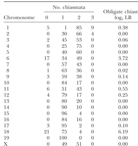
introduced by this convention was ignored. We further as- Crossover and chiasma distributions: The distribu-sumed that all crossovers were observed (i.e., that no double tions of the numbers of crossovers per chromosome are crossovers between typed markers occurred).
displayed in Table 1. The sum of each row in this table
Estimation of chromosome lengths:Estimation of the
ge-is 188, the total number of meioses in the two backcross netic lengths of chromosomes is described above. Standard
panels. Four meiotic products exhibited three cross-errors (SEs) of these lengths were estimated by calculating
the SE of the average number of recombination events ob- overs. Chromosome 19 showed no double crossovers. served for each chromosome. The SEs of chromosome lengths The data in Table 1 were used to estimate, under the ranged from 3.7 to 5.5 cM.
assumption of no chromatid interference, the underly-The genetic lengths derived from the BSB/BSS data were
ing distribution of the number of chiasmata per four-compared to estimates based on counts of chiasmata in C3H/
strand bundle (the distribution p in materials and HeH⫻101/H oocytes by cytological investigation; numbers of
chiasmata were determined for each autosome in 58 oocytes methods) for each chromosome. These estimated dis-(Lawrieet al.1995) and for the X chromosome in 57 oocytes tributions (as percentages) are displayed in Table 2. (Hulte´n et al.1995). SEs of the chiasma-based estimates of
(Note that the estimated SEs of the frequencies were genetic lengths were derived from the reported SDs of the
generally in the range 5–10%.) Chromosomes 1 and 19 numbers of chiasmata.
TABLE 2 TABLE 1
Observed distributions of the number of crossovers Estimated distributions (as percentages) of the number of
chiasmata per meiosis under the assumption per meiotic product
of no chromatid interference
No. crossovers
No. chiasmata
Chromosome 0 1 2 3 Obligate chiasma
Chromosome 0 1 2 3 log2LR
1 53 87 46 2
2 59 95 33 1 1 5 1 85 9 0.38
3 71 92 25 0 2 0 30 66 4 0.00
4 55 99 33 1 3 2 45 53 0 0.06
5 58 105 25 0 4 0 25 75 0 0.00
6 86 78 24 0 5 0 40 60 0 0.00
7 73 95 20 0 6 17 34 49 0 3.72
8 78 93 17 0 7 0 57 43 0 0.00
9 79 91 18 0 8 1 63 36 0 0.02
10 78 103 7 0 9 3 59 38 0 0.14
11 80 88 20 0 10 0 84 17 0 0.00
12 90 90 8 0 11 6 51 43 0 0.55
13 72 108 8 0 12 4 79 17 0 0.25
14 76 108 4 0 13 0 80 20 0 0.00
15 88 98 2 0 14 0 90 10 0 0.00
16 80 101 7 0 15 0 96 4 0 0.00
17 96 91 1 0 16 0 84 16 0 0.00
18 112 74 2 0 17 3 95 2 0 0.10
19 91 97 0 0 18 21 75 4 0 6.19
X 67 98 23 0 19 0 100 0 0 0.00
X 0 49 51 0 0.00
Estimated standard errors for these values are in the range 5–10%. The last column gives the log2LR testing the hypothe-estimated that the majority of meioses have exactly two
sis of an obligate chiasma. The values in some rows do not chiasmata, while chromosome 19 appears to exhibit
ex-sum to 100, due to round-off error. actly one chiasma per meiosis. It should be noted that
these estimated distributions suffer from considerable
imprecision. For example, the 95% confidence interval chromosomes. Note that for chromosome 18, the esti-mated genetic length derived from the BSB/BSS data for the probability of exactly two chiasmata on
chromo-some 1 ranges from 58 to 99%. was quite small relative to that reported byLawrie et al. (1995). The total genetic length of the mouse ge-The estimation procedure allowed us to examine the
hypothesis of an obligate chiasma on each four-strand nome was estimated to be 13.9 M (an average of 27.8 chiasmata per meiosis) on the basis of the BSB/BSS bundle. For most chromosomes, the probability of no
chiasma was estimated to be 0. The last column in Table data and 12.6 M (an average of 25.3 chiasmata per meiosis) on the basis of the chiasma counts.
2 contains the log (base 2) likelihood ratio for testing
the null hypothesis of an obligate chiasma. Large values In Figure 2B, these lengths are plotted against the estimated physical lengths reported by Evans(1996). of the log2 LR indicate evidence against an obligate
chiasma. Only chromosomes 6 and 18 show any depar- The data fromLawrieet al.(1995) showed a biphasic relationship between genetic and physical lengths, with ture from an obligate chiasma. These chromosomes
exhibited a large number of meiotic products with no chromosomes⬍150 Mb having a nearly constant length of 50 cM (one chiasma per meiosis), while for longer crossovers (see Table 1). However, the evidence against
the obligate chiasma hypothesis is not strong. If consid- chromosomes, the genetic lengths increase approxi-mately linearly with physical length. For the lengths eration is made of the 20 statistical tests performed, the
result for chromosome 18 is only marginally statistically derived from the BSB/BSS data (the circles in Figure 2), the biphasic relationship is less clear, although this significant.
In Figure 2A, the estimated genetic lengths of the may be a result of the imprecision in the estimates. It is interesting to note that the SEs of the estimated chromosomes are shown, as derived from the BSB/BSS
data and through cytological inspection of the number genetic lengths derived with the BSB/BSS data are con-siderably larger than those based on chiasma counts, in of chiasmata in oocytes (Hulte´n et al. 1995; Lawrie
et al. 1995). The lengths correspond reasonably well, spite of the fact that the BSB/BSS data comprise 188 meioses, while only 57 (X chromosome) or 58 (au-though the BSB/BSS data gave longer chromosomal
Figure2.—(A) Estimated genetic lengths, with approximate confidence intervals, for each chro-mosome for the BSB/BSS data (䊊) and as re-ported inHulte´net al.(1995) andLawrieet al. (1995), on the basis of counts of chiasmata (䊏). (B) Genetic length vs. physical length for each chromosome.
of the fact that crossover counts are inherently more by Figure 4 inLawrieet al.(1995). The circles and the variable than chiasma counts because of the sampling tick marks below and to the left indicate the locations of chromatids (each chiasma involves two of the four of the pair of crossovers on meiotic products with exactly possible strands). Letndenote the number of chiasmata two crossovers. Circles above the dotted diagonal line for a chromosome, and let m denote the number of correspond to crossovers separated by⬍20 cM. Ten out crossovers on that chromosome in a random meiotic of the 323 pairs of crossovers were separated by⬍20 cM. product. Then, under no chromatid interference, The presence of so few points above this line indicates strong positive crossover interference in the mouse. If var(m)⫽E[var(m|n)]⫹var[E(m|n)]
there were no crossover interference, the points would be uniformly distributed over the triangle defined by
⫽E(n/4)⫹var(n/2)
the solid diagonal line, and so we would expect 145 out
⫽[2L⫹var(n)]/4,
of the 323 pairs of crossovers to be separated by⬍20 cM. Note that the ticks on the right indicate the locations of whereL⫽E(n)/2 is the genetic length of the
chromo-markers on the genetic map; the maps are quite dense, some (in morgans). This is dominated by the genetic
though there remain a number of gaps. The ticks at length,L, since var(n)⬍ 0.1 (seeLawrieet al.1995),
the top indicate the locations of crossovers on meiotic while 2Lis in the range 1–2. Counts of crossovers thus
products with exactly one crossover; these are approxi-provide less precise estimates of the genetic lengths
mately evenly distributed. The x’s indicate the locations of chromosomes. On the other hand, recombinational
of crossovers on the four triple-crossover meiotic prod-information may provide more precise estimates of the
ucts. Note that these crossovers are widely spaced, with locations of crossovers, which are of principal interest
the closest pair of crossovers separated byⵑ18 cM. in an analysis of interference.
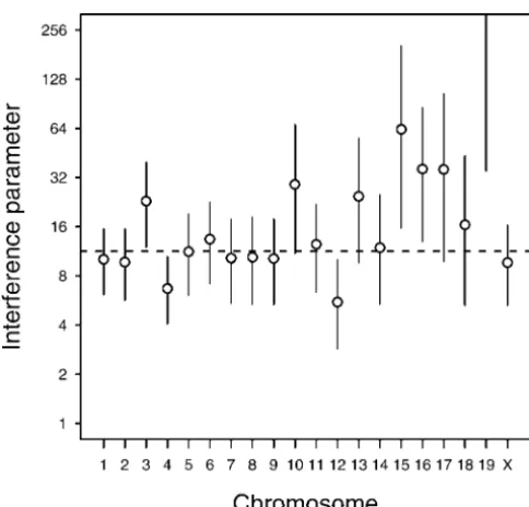
Levels of interference:Figure 4 displays the chromo-Figure 3 provides a detailed view of the crossover
Figure 3.—Crossover lo-cations for all chromo-somes. Each square repre-sents a chromosome, with the centromere at the top and left and the telomere at the bottom and right. Ticks on the right indicate the lo-cations of the genetic mark-ers. The circles indicate the locations of the pair of crossovers on meiotic prod-ucts exhibiting exactly two crossovers, with the location of the proximal and distal crossovers shown below and to the left, respectively. Cir-cles above the dotted diag-nonal line are crossovers separated by⬍20 cM. The locations of crossovers on meiotic products that ex-hibit exactly one crossover are shown at the top. The x’s above chromosomes 1, 2, and 4 indicate the loca-tions of crossovers on triple-crossover meiotic products.
for the gamma model, with likelihood support intervals ference than the other chromosomes. These were the only chromosomes exhibiting more than one pair of (the values of for which the likelihood was within a
factor of 10 of its maximum) indicating plausible values crossovers separated by⬍20 cM (see Figure 3). A pair of crossovers on chromosome 12 were separated by only of . A horizontal line is plotted at ˆ ⫽ 11.3 (SE ⬇
0.7), the estimate obtained after pooling data across 10 cM.
A likelihood-ratio test to assess interchromosomal chromosomes. Note that for chromosome 19, none of
the 188 meiotic products exhibited more than one cross- variation in the level of interference indicated strong evidence for such variation (P⬇10⫺5). Figure 5 displays over, and soˆ⫽∞; the lower bound of the likelihood
support interval was 35. These data show clear evidence the estimates ofas a function of chromosome length. Smaller chromosomes are seen to generally exhibit for interference on all chromosomes. The no
interfer-ence model corresponds to the value ⫽1; the likeli- stronger levels of interference, although the confidence intervals for the chromosome lengths and levels of inter-hood support intervals for for all chromosomes are
well above the value 1. ference are wide, indicating considerable uncertainty in each.
inter-Figure4.—Estimates of the interference parameterfrom the gamma model for each chromosome, with approximate confidence intervals. A horizontal line is plotted at the pooled estimate of. Note that chromosome 19 gaveˆ⫽∞.
Figure 6 displays, for chromosomes 1–4, the
distribu-tion of the distance between crossovers on meiotic prod- Figure6.—Observed distributions of the distance between crossovers for meiotic products exhibiting exactly two cross-ucts exhibiting exactly two crossovers. The solid curves
overs. (nindicates the number of such products.) The solid correspond to the fitted distributions for the gamma
and dashed curves correspond to the fitted distributions under model. The dashed curves correspond to the fitted dis- the gamma and no interference models, respectively. tributions in the case of no crossover interference. The
dearth of closely spaced crossovers (also seen in Figure
3) indicates strong evidence for positive crossover inter- two crossovers; the histogram at the top left of Figure ference. The gamma model provides a reasonably good 6 does not deviate significantly from the fitted curve fit to these data. While the fit is not perfect, this is under the gamma model.
in part the result of a paucity of data. For example, chromosome 1 showed 46 meiotic products with exactly
DISCUSSION
The results of this study provide strong genome-wide evidence for positive crossover interference in the mouse. A gamma model with ⫽7.6 has a map function that corresponds approximately to the Carter-Falconer map function (ZhaoandSpeed1996). The pooled estimate offor these data was 11.3, indicating that the average strength of crossover interference in the mouse may be stronger than that implied by the Carter-Falconer map function. Note, for comparison, that ⫽ 1 under no interference, andˆ⫽4.3 is the estimated level of inter-ference in humans (BromanandWeber2000). Cross-over interference in the mouse appears to be extremely strong.
It is important to emphasize that we analyzed a pair of reciprocal interspecific backcrosses with a common female F1 parent. Thus these conclusions may not ex-Figure5.—Estimates of the interference parameterfrom
actly model either male meiosis or crosses using other the gamma model, plotted against chromosome length.
Verti-mouse strain combinations. cal and horizontal segments indicate approximate confidence
We assumed that the markers were in the correct order of the interference parameter is infinite when no meiotic products exhibit more than one crossover, the and that the intermarker distances were known exactly.
We assumed that all crossovers were observed and that bias of the MLE is also infinite, unless one conditions on the presence of at least one meiotic product with the imprecision in the localization of crossovers was
unimportant. Finally, we assumed that the level of inter- more than one crossover.) However, it does not appear that this bias is sufficient to explain the relationship ference was constant, relative to genetic distance, along
each chromosome. (It will be valuable to revisit this between chromosome size and level of interference ob-served in these data.
work once the physical locations of markers become
available, since interference may act on the physical The observed numbers of crossovers per chromosome allowed us to investigate the hypothesis of an obligate scale. The inhomogeneity in recombination frequency
along chromosomes will make such an investigation dif- chiasma per four-strand bundle. Only two chromosomes (6 and 18) provided any evidence against an obligate ficult, but also more interesting.)
In spite of these approximations, the estimated levels chiasma, and this evidence was weak. We conclude that these data are consistent with the obligate chiasma hy-of interference are likely reasonable, though their
esti-mated SEs are somewhat too small. For example, chro- pothesis.
It is interesting to note the apparent relationship be-mosome 12 showed a lower level of interference than
any other chromosome (ˆ ⫽ 5.5), largely the result of tween frequency of recombination and degree of inter-ference: the mouse and human genomes are similar in two tight double crossovers, including a pair of
cross-overs separated by only 10 cM (see Figure 3). If the size, but the human has a higher crossover frequency and a lower level of interference (BromanandWeber estimated genetic distance between these crossovers had
been larger, the estimated level of interference on chro- 2000). The human genome has been estimated to be ⵑ44 M (female) or 27 M (male), or an average of 35.8 M mosome 12 would be stronger. Estimates of the
interfer-ence parameter are clearly sensitive to the distance be- (Bromanet al.1998). The mouse genome size estimated from these interspecific backcross data is 13.9 M. (The tween tightly spaced double crossovers.
Our results rely, in part, on the appropriateness of degree of difference between sex-specific recombina-tion frequencies varies among mouse strains, but is the gamma model. While the gamma model provides a
reasonable fit to these data (see Figure 6), it fails to much lower than in humans.) Remarkably, the ratio of the estimated genetic lengths of the human and mouse capture all of the biological details of the recombination
process. For example, it does not require the presence genomes (35.8 M human/13.9 M mouse⫽2.6) is the reciprocal of the ratio of the estimated interference of at least one chiasma on the four-strand bundle. The
gamma model should be viewed as a device for estimat- parameters, (11.3 mouse/4.3 human ⫽ 2.6). (This observation should be considered with great care, as ing the strength of crossover interference. While more
elaborate mathematical models might conform better the interference parameter is measured on an arbitrary scale.) However,BromanandWeber(2000) found no to what is known about the biological mechanism of
the recombination process, the data are not sufficient significant difference in the degree of interference be-tween the sexes in humans, while there is a 1.6-fold to discriminate between such models, and the estimated
levels of interference would likely be little changed. difference in the frequency of recombination. This sug-gests that the control of interference may be species We observed some evidence for variation in
interfer-ence between chromosomes, with smaller chromosomes specific, with additional sex-specific control of recombi-nation in some animals.
showing a greater level of interference (see Figure 5).
This is in contradiction to previous results on the rela- The mouse backcross data used here give an estimate of an average chiasma frequency of 27.8 per genome. tionship between chromosome size and the strength of
interference; Kaback et al. (1999) reported that, in This agrees well with frequencies observed by others on the basis of direct cytological observations: 25.3 average yeast, smaller chromosomes exhibit alowerlevel of
inter-ference. The imprecision in the estimates of both the chiasmata per cell reported byHulte´nand colleagues (Hulte´net al.1995;Lawrieet al.1995) and 27.5 chias-levels of interference and the genetic lengths of the
chromosomes makes the assessment of this relationship mata per cell observed byPolani(1972). The discrep-ancy between the estimated genetic lengths based on difficult.
Further, the estimates of the levels of interference for BSB/BSS data and those reported by Lawrie et al.
(1995) was greatest for the small chromosomes. Note small chromosomes appear to be subject to a positive
bias (i.e., the observed estimates are likely too large). that the greater level of recombination in these data is the opposite of what one would expect in a cross be-We conducted a small computer simulation study (data
not shown) to investigate the possibility of bias for differ- tween such divergent strains. With 20 centromeres, 28 chiasmata approaches the minimum necessary to ensure ent levels of interference and different chromosome
lengths. For chromosomes⬍60 cM, the bias isⵑ0.1–0.3 proper disjunction at meiosis. Thus it can be predicted that the mouse may have one of the highest levels of on the log2scale; for large chromosomes, the bias was
Lyon, S.Rastanand S. D. M.Brown. Oxford University Press, ratios of recombination frequency to centromere count
London.
have very low or no interference (seeSymandRoeder Fisher, R. A., M. F. LyonandA. R. G. Owen, 1947 The sex
chromo-1994). somes in the house mouse. Heredity1:335–365.
Foss, E. J., andF. W. Stahl, 1995 A test of a counting model for Recently, synaptonemal complex proteins have been
chiasma interference. Genetics139:1201–1209.
implicated in the control of crossover interference. In Foss, E. J., R. Lande, F. W. StahlandC. M. Steinberg, 1993 Chi-both yeast and tomato, interference has been shown asma interference as a function of genetic distance. Genetics133:
681–691. to be limited to portions of chromosomes involved in
Hulte´n, M. A., C. TeaseandN. M. Lawrie, 1995 Chiasma-based synaptonemal complexes (ChuaandRoeder1997). In genetic map of the mouse X chromosome. Chromosoma 104: yeast, null mutations in the synaptonemal complex pro- 223–227.
Kaback, D. B., D. Barber, J. Mahon, J. LambandJ. You, 1999 Chro-teins tam1 and zip1 show no reduction in recombination
mosome size-dependent control of meiotic reciprocal recombina-frequency but a marked reduction in interference (Sym tion inSaccharomyces cerevisiae: the role of crossover interference. andRoeder1994;ChuaandRoeder1997). The results Genetics152:1475–1486.
Karlin, S., andU. Liberman, 1994 Theoretical recombination pro-of our study suggest that a comparison pro-of mouse and
cesses incorporating interference effects. Theor. Popul. Biol.46:
human synaptonemal complex proteins may reveal in- 198–231.
sights into the mechanism of modulation of interfer- Kingsley, D. M., N. A. JenkinsandN. G. Copeland, 1989 A molecu-lar genetic linkage map of mouse chromosome 9 with regional ence.
localizations for the Gsta, T3g, Ets-1 and Ldlr loci. Genetics123:
The backcross panels established by Rowe et al. 165–172.
(1994) are a valuable resource, both for the high-density Lander, E. S., andP. Green, 1987 Construction of multilocus ge-netic linkage maps in humans. Proc. Natl. Acad. Sci. USA84:
genetic maps of the mouse genome that they provide
2363–2367.
and for the analysis of crossover interference described Lawrie, N. M., C. Teaseand M. A. Hulte´n, 1995 Chiasma fre-herein. Our analysis relied on high-quality, high-density quency, distribution and interference maps of mouse autosomes.
Chromosoma104:308–314. genotype data, which can be obtained only through
Lin, S., andT. P. Speed, 1996 Incorporating crossover interference careful curation, including the resolution of apparent into pedigree analysis using the2model. Hum. Hered.46:315– genotyping errors. While data on substantially more 322.
McPeek, M. S., and T. P. Speed, 1995 Modeling interference in meioses, combined with information on the physical
genetic recombination. Genetics139:1031–1044.
locations of genetic markers, will provide a more de- Muller, H. J., 1916 The mechanism of crossing-over. Am. Nat.50: tailed view of the recombination process, this study and 193–221, 284–305, 350–366, 421–434.
Munz, P., 1994 An analysis of interference in the fission yeast
Schizo-these backcross panels have succeeded in providing the
saccharomyces pombe.Genetics137:701–707.
first complete characterization of crossover interference Ott, J., 1996 Estimating crossover frequencies and testing for nu-in the mouse. merical interference with highly polymorphic markers, pp. 49–63 inGenetic Mapping and DNA Sequencing:IMA Volumes in Mathematics
S´aunak Sen provided valuable advice on Figure 3. and Its Applications, Vol. 81, edited by T.Speedand M. S. Water-man. Springer-Verlag, New York.
Polani, P. E., 1972 Centromere localization at meiosis and the posi-tion of chiasmata in the male and female mouse. Chromosoma
36:343–374. LITERATURE CITED
Roeder, G. S., 1997 Meiotic chromosomes: it takes two to tango. Blank, R. D., G. R. Campbell, A. CalabroandP. D’Eustachio, Genes Dev.11:2600–2621.
1988 A linkage map of mouse chromosome 12: localization of Rowe, L. B., J. H. Nadeau, R. Turner, W. N. Frankel, V. A. Letts Igh and effects of sex and interference on recombination. Genet- et al., 1994 Maps from two interspecific backcross DNA panels ics120:1073–1083. available as a community genetic mapping resource. Mamm. Ge-Broman, K. W., andJ. L. Weber, 2000 Characterization of human nome5:253–274.
crossover interference. Am. J. Hum. Genet.66:1911–1926. Sturtevant, A. H., 1915 The behaviour of the chromosomes as Broman, K. W., J. C. Murray, V. C. Sheffield, R. L. WhiteandJ. L. studied through linkage. Z. Indukt. Abstammungs Vererbungsl.
Weber, 1998 Comprehensive human genetic maps: individual 13:234–297.
and sex-specific variation in recombination. Am. J. Hum. Genet. Sym, M., andG. S. Roeder, 1994 Crossover interference is abolished
63:861–869. in the absence of a synaptonemal complex protein. Cell79:283– Carter, T. C., andD. S. Falconer, 1951 Stocks for detecting linkage 292.
in the mouse, and the theory of their design. J. Genet.50:307– Weeks, D. E., J. OttandG. M. Lathrop, 1994 Detection of genetic
323. interference: simulation studies and mouse data. Genetics136:
Ceci, J. D., L. D. Siracusa, N. A. JenkinsandN. G. Copeland, 1217–1226.
1989 A molecular genetic linkage map of mouse chromosome Weinstein, A., 1936 The theory of multiple-strand crossing over. 4 including the localization of several proto-oncogenes. Geno- Genetics21:155–199.
mics5:699–709. Yu, K., andE. Feingold, 2001 Estimating the frequency distribution Chua, P. R., andG. S. Roeder, 1997 Tam1, a telomere-associated of crossovers during meiosis from recombination data. Biometrics
meiotic protein, functions in chromosome synapsis and crossover 57:427–434.
interference. Genes Dev.11:1786–1800. Zhao, H., andT. P. Speed, 1996 On genetic map functions. Genetics Cox, D. R., 1962 Renewal Theory. Methuen, London. 142:1369–1377.
Dempster, A., N. LairdandD. Rubin, 1977 Maximum likelihood Zhao, H., M. S. McPeekandT. P. Speed, 1995a Statistical analysis from incomplete data via the EM algorithm. J. R. Stat. Soc. Ser. of chromatid interference. Genetics139:1057–1065.
B39:1–22. Zhao, H., T. P. SpeedandM. S. McPeek, 1995b Statistical analysis Egel, R., 1995 The synaptonemal complex and the distribution of of crossover interference using the chi-square model. Genetics
meiotic recombination events. Trends Genet.11:206–208. 139:1045–1056. Evans, E. P., 1996 Standard idiogram, p. 1446 inGenetic Variants