Random matrix approaches to open quantum systems

(1)

Random matrix approaches to open

quantum systems

Henning Schomerus

(2)

(3)

1 Introduction

1.1 Welcome

Open quantum systems come in two variants. The first variant (on which we will focus more) are scattering systems in which the dynamics allow particles to enter and leave (Newton, 2002; Messiah, 2014). One then normally defines a scattering region, out-side of which particles move free of any external forces or interactions. This situation is realised (at least to some level of approximation) in many decay or radiation pro-cesses (Weidenm¨uller and Mitchell, 2009), but is also useful to describe phase-coherent transport in mesoscopic devices (Datta, 1997; Beenakker, 1997; Blanter and B¨uttiker, 2000; Nazarov and Blanter, 2009) or photonic structures (Cao and Wiersig, 2015). The second variant (which we will encounter only briefly) are interacting systems in which the studied dynamical degrees of freedom are influenced by other degrees of freedom in the environment (Breuer and Petruccione, 2002). This situation spans from the quantum-statistical foundations of thermodynamics (Gemmer et al., 2010) to the description of decoherence (Weiss, 2008), with ample applications to quantum optics (Carmichael, 2009), quantum-critical phenomena (Sachdev, 1999) and quantum information processing (Nielsen and Chuang, 2010).

While these two scenarios of openness are in many ways quite distinct, they have some important features in common—in particular, in both scenarios we are led to restrict our attention to a subsystem, while the processes that are involved often are very complex (meaning that we have no realistic handles to describe them in detail), be it due to underlying classical chaos, disorder, or uncontrolled interactions. Taken together, these features lay the foundations for a statistical description where individ-ual systems are replaced by an appropriate ensemble. These ensembles are typically formulated in terms of effective models, e.g., for the Hamiltonian, the scattering ma-trix, or the density mama-trix, in which only the fundamental symmetries and the most essential time and energy scales are retained. Quantitative predictions then follow from explicit calculations and often turn out to be universal, i.e., applicable to generic representatives of the ensemble.

(5)

2 Introduction

With this selection of topics, we hope to provide a useful bridge to the many excel-lent advanced sources, including the monographs and reviews mentioned above, which contain detailed expositions of the random-matrix calculations and further applica-tions not covered here. In the remainder of this introduction, we provide some basic background.

1.2 Primer

These lectures were delivered to a mixed audience of mathematicians and physicists. To establish some common language, let us first review some basic notions of quantum mechanics (Peres, 2002). This also gives us the opportunity to pinpoint the funda-mental origins of the mathematical concepts and physical phenomena that we will encounter throughout these notes—and further explain what these notes are really about.

Let us recall, then, that quantum mechanics describes the physical states of a system in terms of vectors|ψi,|φi, . . .in a complex Hilbert spaceH. The superposition principle means that the vectors can be freely combined to yield new physical states α|ψi+β|φi,α, β∈_C. All vectorsα|ψithat differ only by a multiplicative factorα6= 0 describe the same physical state, which is often exploited to impose the convenient normalizationhψ|ψi= 1. Following physics convention, we here use (what we term) the scalar product withhφ|(αψ+βχ)i=αhφ|ψi+βhφ|χi,hψ|φi=hφ|ψi∗_,_h_ψ_|_ψ_i_>₀ unless|ψi= 0, where ∗ denotes complex conjugation. Two states withhφ|ψi= 0 are called orthogonal, and a discrete basis withhn|mi=δnm is called orthonormal. For a continuous basis, this is replaced byhx|x0i=δ(x−x0) with Dirac’s delta function. In a given basis, states can be expanded as|ψi=P

nψn|niwhereψn=hn|ψi, with the sum replaced by an integral when the basis is continuous.

Observables are represented by hermitian linear operators ˆA, with ˆA|ψi ≡ |Aψˆ i ∈ Hsuch thathφ|Aψˆ i=hAφˆ |ψi. According to the measurement axiom, these operators predict physical observations via the expectation valuesEψ(A) =hψ|Aψˆ i/hψ|ψi, which in reality are obtained by averaging the outcomes of experiments on systems in the same quantum state. The associated uncertainty (variance) is obtained from ∆A = [Eψ(A2)− Eψ2(A)]

1/2_{, which in general is finite. Denoting by}_E

a =Pn|ψa,nihψa,n|the projector onto states that guarantee an outcomeawith vanishing uncertainty ∆A= 0, one finds that these are eigenstates with ˆA|ψa,ni = a|ψa,ni. In a general state, the probability of these outcomes|ψiare thenP(a) =hψ|Ea|ψi/hψ|ψi; no outcomes other than the associated eigenvalues are allowed. Beyond this probabilistic description, outcomes of individual experiments are unpredictable. Finally, the measurement axiom stipulates that right after the measurement with an outcome a, the quantum system acquires the stateEa|ψi.

Adopting the conventional Schr¨odinger picture, the time dependence of the quan-tum state arises from the Schr¨odinger equation

i~d

(6)

Open systems 3

|ψ(t)i = Û(t, t0)|ψ(t0)i, where Û(t, t0) is a unitary operator ( Û is unitary if always

In order to describe the incoherent mixture of normalised quantum states|ψnione introduces the density matrix (statistical operator) ˆρ=P

npn|ψnihψn|with positive weights pn summing to Ppn = 1, so that tr ˆρ= 1. The expectation valuesEρ(A) = tr ( ˆAρ) =ˆ P

npnEψn(A) are a combination of the quantum-mechanical average in each

quantum state and the classical average over the weights pn. The density operator is hermitian and positive semidefinite, and for a pure state (with only one finitepn= 1) becomes a projector, ˆρ2 _{= ˆ}_{ρ. To capture the departure from this situation one can} consider the purityP = tr ˆρ2_{, which equals unity only for a pure state, as well as the} von Neumann entropyS =−tr ˆρln ˆρ, which vanishes for a pure state.

1.3 Open systems

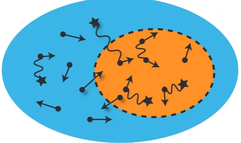
The superposition principle mentioned above is the origin of wave-like interference effects, the complexity of which we will aim to capture in a statistical description. To provide the states with some structure, we can often think of the state space being divided into sectors (which we here call regions), H =H1⊕ H2. We then can start to talk about local and non-local processes, within or between the regions, and intro-duce basic notions such as the exchange of particles or energy. An additional layer of complexity is added when we can view the system as being composed of separate degrees of freedom (which we here call parts). The Hilbert space then takes the form of a tensor productH=H1⊗ H2, with proper symmetrization or antisymmetrization if the parts are, in a physical sense, indistinguishable (e.g., when they describe iden-tical bosonic or fermionic particles). Separable states are of the form|φi ⊗ |χi, while superpositions of such states lead to quantum correlations (entanglement) that deeply enrich the behaviour of interacting systems. Based on these elements of structure, let us now agree, within the confines of these notes, on two notions of open quantum systems. These are systems in which we can naturally focus on some region or part

(7)

[image:7.595.116.364.167.314.2]

4 Introduction

Fig. 1.1 Quantum systems couple to their environment by the exchange of particles and en-ergy, and thereby by processes connected to the kinetic freedom of motion and the interactions of the various components.

1.4 Preview

With these concepts at hand, we can now define our mission—to provide a statistical description of open quantum systems in terms of random matrices. This succeeds in situations where we can apply statistical considerations also to the complex dynam-ics in the region or part of interest, with constraints only arising from fundamental symmetries. We describe both settings in their purest incarnation.

(i) Our main focus is the elastic scattering of a non-interacting particle, which can undergo complex dynamics in the region of interest but enters and leaves in pre-dictable ways. This is quantified in terms of the amplitudes of the incoming and out-going waves, which are linearly related by a unitary scattering matrixS. As this pure setting is stationary, we can work in the energy domain, while time scales follow when we consider variations in energy. This setting also covers decay processes, where we initially confine the particle within the region of interest—effectively, this is described by a non-hermitian Hamiltonian, with eigenvalues that coincide with the poles of the scattering matrix.

(ii) In a small detour at the end of these notes, we consider purely interacting systems, with localized degrees of freedom that cannot move but evolve under the influence of their mutual environment. We quantify this in terms of a reduced density matrix, a hermitian, positive semidefinite matrix which represents the quantum state when one ignores the other degrees of freedom. We again assume complex internal dynamics, and consider entropies that quantify entanglement.

(8)

Preview 5

(9)

2 Foundations of random-matrix

theory

In this chapter we review a range of classical random-matrix ensembles against the backdrop of closed-system behaviour, which informs the subsequent applications to open systems.

2.1 Random Hamiltonians and Gaussian hermitian ensembles

Random-matrix descriptions in quantum mechanics naturally start out with consider-ations of closed systems. In this setting, the main object of interest is the Hamiltonian

ˆ

H, whose eigenvalues give the energy levels. The energy spectrum can be characterised very neatly if one manages to identify a number of conserved quantities that commute with the Hamiltonian and amongst each other; considering joint eigenstates of these quantities helps to bring some order to the spectrum. In sufficiently complex systems, however, effects such as chaotic or diffractive scattering and interactions eliminate all conserved quantities, and the energy spectrum lacks any apparent regularities. It is natural to compare the resulting features with the case where the Hamiltonian can be considered as random. This was first proposed in the 1950’s by Wigner (1956), who sought ways to analyse resonances in heavy nuclei. The idea is to focus on a suitable energy range, where the local spectral properties can then be studied by replacing the full Hamiltonian with a randomly chosenM×M-dimensional hermitian matrix (the limitM → ∞can be imposed later on).

The quality of this descriptions depends on the identification of a suitable random-matrix ensemble. To achieve this task we are allowed to incorporate any general feature of the system. These are, in particular, fundamental symmetries, rough geometric constraints such as dimensionality, as well as natural time and energy scales.

(10)

Random Hamiltonians and Gaussian hermitian ensembles 7

after a short time Terg, which in particularly is much shorter than the Heisenberg time TH = 2π~/∆ (the minimal observation time at which individual energy levels can be resolved). Examples where this is realised are sufficiently featureless disordered (Efetov, 1996) or classically chaotic systems (St¨ockmann, 2006; Haake, 2010). The short-ranged level statistics then becomes universal, and can be captured by ensem-bles with Gaussian statistics of the matrix elements (Mehta, 2004; Guhret al., 1998; Haake, 2010; Forrester, 2010).

2.1.1 Time-reversal symmetry and the Wigner-Dyson ensembles

We start by considering the role of time reversal (Dyson, 1962a; Haake, 2010), in-stituted by an anti-unitary operator T fulfilling hTφ|Tψi = hψ|φi = hφ|ψi∗_{, which} consequently may square toT2_{= 1 or}_T2₌₋_1.

If the Hamiltonian obeys a time-reversal symmetryTHT−1₌_H _with_T2_{= 1, we} can adopt an invariant basis |ni in which hTn|ψi= hn|ψi for any |ψi. This implies

hn|Tψi=hn|ψi∗_{, so that the time-reversal operation}_T ₌_K _{amounts to the complex} conjugation of the expansion coefficients ψn = hn|ψi of any state. In this basis the matrix elements Hlm = hl|Hˆ|mi = hTl|HˆT |mi = Hlm∗ are real, while hermiticity implies that the matrix is symmetric, Hml =Hlm. This is known as theorthogonal symmetry class (OE), to which we associate the symmetry index β= 1.

In absence of any time-reversal symmetry, matrix elements of the Hamiltonian are in general complex, withHlm =Hml∗ because of hermiticity, which defines theunitary symmetry class (UE) with symmetry indexβ = 2.

[image:10.595.100.497.501.701.2]

If we have a time-reversal symmetry THT−1 ₌ _H _with _T2 ₌ ₋_{1 (symplectic} symmetry class SE with symmetry index β = 4), we can adopt a basis arranged in pairs|ni=T |n¯i, so that the Hilbert space dimension 2M must be even. In this basis,

Table 2.1 Fundamental symmetries of hermitian random-matrix ensembles

symmetries constraints realization (H_mn∗ =Hnm)

no symmetries none besidesH =H† Hnm∈C

T =K H∗=H Hnm∈R

T = ΩK H∗= ΩHΩ−1 Hnm∈H

C=K H∗=−H Hnm∈iR

C=K, T = ΩK H∗=−H= ΩHΩ−1 Hnm=−σyHnmσy∈H

C= ΩK H∗=−ΩHΩ−1 Hnm∈iH

C= ΩK,T =K H∗₌_H ₌₋_ΩH_Ω−1 _H

nm=−σyHnmσy∈iH

X =τz≡diag (1M1,−1M2) H =−τzHτz H =

0 A A† 0

,Anm∈C

X =τz,C=K (T =X C) H =−τzHτz=−H∗ H =

0 A A† 0

,Anm∈iR

X =τz,C= ΩK(T =X C) H =−τzHτz=−ΩH∗Ω−1 H =

0 A A† 0

(11)

8 Foundations of random-matrix theory

T = ΩKwhere Ω =iσy⊗1M, while the blocks

Hlm Hlm¯ H¯_lm H¯_l_m_¯

=alm1+iblmσx+iclmσy+

idlmσz∈Hcan be reinterpreted as quaternions, with real coefficientsalm, blm, clm, dlm and Pauli matricesσr. Hermiticity requires thatalm =aml forms a symmetric matrix while blm = −bml, clm = −cml, dlm = −dml are antisymmetric. Expressed as an M×M-dimensional matrix of quaternions,H =H is then seen to be quaternion self-conjugate, where by definition (H)lm=Hml=aml1−ibmlσx−icmlσy−idmlσz. For such a matrix, all energy levels appear in degenerate pairs, a phenomenon known as Kramers degeneracy; in all following considerations we count each pair as a single level. In keeping with this, the quaternion trace is defined as trH =P

nann(so differs by a factor of two from the conventional trace), and the quaternion determinant is similarly modified to maintain the relation det expA= exp trA, which makes it equivalent to a Pfaffian (Dyson, 1970).

The symmetry index β = 1,2,4 mentioned above counts the real degrees of free-dom in the matrix elements. The corresponding notions of orthogonal, unitary and symplectic symmetry classes refer to the transformationsH =U D U†,D= diag(En) that diagonalise these Hamiltonians. Forβ= 1 the matrixU is orthogonal,U UT = 1, and hence belongs to the group O(M); for β = 2 U ∈ U(M) is a unitary matrix with U U† _{= 1, and for} _β _{= 4 the matrix is unitary symplectic,} _U _∈ _Sp(2M_{) with} U U = 1. This ‘threefold way’ can be further justified within representation theory (Dyson, 1962c).

Within these three Wigner-Dyson classes, the universal spectral features encoun-tered in ergodic systems are captured by the Gaussian orthogonal, unitary, or symplec-tic ensemble (GOE, GUE, GSE), where the Hamiltonian obeys a probability density of the formP(H)∝exp(−cβtrH2) withcβ=βπ2/4M∆2. The spectral statistics can then be determined from the joint probability distribution

P({En})∝ Y

n<m

|En−Em|β Y

k

exp(−cβEk2), (2.1)

which follows by a change of variables from the Hamiltonian to its eigenvalues and eigenvectors. This result can be obtained by sophisticated methods in the language of differential geometry (Forrester, 2010), but in this specific incarnation also follows from elementary means and then acquires a simple geometric meaning. Given that dH =dU DU†+U dDU†−U DU†U U†, consider the squared line element

X

lm

|dHlm|2= tr (dHdH) = tr (dXD−DdX)†(dXD−DdX) + X

m

(dEm)2, (2.2)

whereD containsM real parameters (the eigenvalues) while dX=−iU†dU depends onM(M−1)/2 real, complex or quaternion parameters in the set of eigenvectors. The latter parameters can be associated with the rotations R(nm)_{in the}_nm _{plane of the} diagonalised system, spanned by the eigenvectors with eigenvaluesEnandEm. Each of these rotations then translates into a line element in the space of Hamiltonians of length

∝ |En−Em|β, where the power arises from the fact that the rotation is parameterised byβ real variables. (In particular, if we rotate the basis in a degenerate subspace the Hamiltonian does not change.) Hencedµ(H)∝ Q

(12)

whereµ(U) is the Haar measure arising from the formdX in the corresponding group of transformations. This measure is uniquely defined by the requirement that it is invariant underU →V0U V for any fixedV, V0 form the same group.

The main characteristics of (2.1) is a universal degree of level repulsionP(s)∼sβ for small level spacingss=|En−Em| in the bulk of the spectrum. This feature was first realised by Wigner, who put forward the famous surmise P(s)∼ sβexp(−cs2) with a suitable scale factor c (Porter, 1965). As it turned out, this surmise is exact only forM = 2, but provides a very accurate estimate for anyM. The exact result can be established by the method of orthogonal polynomials (here based on Hermite polynomials), which provides the complete set of correlation functions (Mehta, 2004). When applied to a particular system, these correlations describe the short-ranged statistics in the bulk, i.e., over sufficiently small spectral ranges where the mean level spacing ∆ is well defined (possibly, after some unfolding of the spectrum). In particular, the amount of level repulsion is considered as a prime indicator of whether a system displays the required ergodic dynamics, as further discussed in Chapter 5.

The mean level spacing itself is not universal; in real systems it varies systematically with energy, but for any comparison we wish to have it well defined in any given ensemble. In the Gaussian ensembles, this is guaranteed by the form of the eigenvalue density, which for large matrix dimensions M → ∞ approaches the famous Wigner semicircle law (Wigner, 1958)

ρ(E) = 1 ∆

q

1−E2_/E2

0 for|E|< E0= 2M∆/π. (2.3) A derivation of this classical result is given in the Appendix. It reveals that ∆ = 1/ρ(0) is the mean level spacing at E = 0, defining the middle of the bulk around which we then determine the universal spectral features. Universal level statistics are also encountered around the spectral edges±E0, whose actual positions are again system specific.

2.1.2 Chiral symmetry

Additional positions within the spectrum deserve dedicated attention when further symmetries come into play. In particular, this is encoutered when the Hamiltonian is antisymmetric under a suitable unitary or antiunitary transformation, an effect which often occurs in single-particle descriptions of fermions. Energy levels then appear in pairs En, E˜n = −En, with the possible exception of levels pinned to the spectral symmetry pointE= 0.

IfXHX =−H with a unitary involutionX (such thatX2_{= 1), we talk of a chiral} symmetry (Verbaarschot, 1994; Verbaarschot and Wettig, 2000). For a finite system of dimension M =M1+M2, we can choose X = diag (1M1,−1M2)≡τz, so that the

Hamiltonian takes a block form

H =

0 A A† 0

(2.4)

(13)

The chiral symmetry arises in elementary particle physics (Verbaarschot and Wet-tig, 2000; Akemann, 2017), but can also be realised as an effective symmetry in elec-tronic (Brouwer et al., 2002), superconducting (Fu and Kane, 2008) and photonic systems (Schomerus and Halpern, 2013; Luet al., 2014; Poliet al., 2015). Given the structure (2.4), the symmetry generally applies to systems with two sublattices, termed A and B, when the couplings within each isolated sublattice vanish (Sutherland, 1986). The mentioned electronic and photonic implementations naturally extend this idea to suitably coupled subsystems.

An interesting aspect of these classes is the appearance of topological invariants, associated with the number of eigenenergies pinned to the symmetry point (Lieb, 1989; Verbaarschot, 1994; Brouwer et al., 2002). For a Hamiltonian of the form (2.4) with some finiteν = M2−M1 (so that A is not square), there are at least |ν| such zero modes. Ifν <0 the associated eigenstates are of the formψ= (ψA,0)T withA†ψA= 0, while forν >0 we haveψ= (0, ψB)T withAψB= 0. The remaining paired levels with finite energy can be determined from the positive definite matrixA†AorAA†, whose eigenvalues are given byE2

n.

In combination with considerations of time-reversal symmetry one can now define chiral orthogonal, unitary or symplectic symmetry classes (chOE, chUE, chSE) (Ver-baarschot, 1994; Verbaarschot and Wettig, 2000; Akemann, 2017), which are again associated with a symmetry indexβ= 1,2,4. TakingAas a random matrix with real, complex, or quaternion entries andP(A)∝exp(−cβtrA†A) then leads to the Gaus-sian chiral ensembles (chGOE, chGUE, and chGSE), for which the positive energy levels in each pair follow the joint distribution

P({En})∝ Y

n<m,En,m>0

|E_n2−E_m2|β Y

k,Ek>0

E_k(|ν|+1)β−1exp(−cβE2k). (2.5)

The termsE2

n−E2m= (En−Em)(En+Em) include the repulsion from the negative-energy levels, whileE_k(|ν|+1)β−1 includes the repulsion from the mirror level at E˜_k =

−Ek and from the zero modes. This modified repulsion follows again from the geo-metric argument above, where the subspace to be explored by the rotations R(nm) corresponds to the caseM1=|ν|+ 1,M2= 1. In this space,Abecomes a vector and the eigenvalues and the squared eigenvaluesEn2 =E2˜n=|A|

2 _{obey a}_χ2 _{distribution.}

These modifications affect the eigenvalue density around E= 0 over a range of a few level spacings,

ρ(E)− |ν|δ(E)∝ |E|(|ν|+1)β−1 _{for small}_|_E_|_, _(2.6) which now becomes a universal spectral characteristic of the system. For a macroscopic number of zero modes withM2 M1 1, the repulsion yields a hard gap around the symmetry point, corresponding to the mean density

ρ(E) = π M1∆2E

q

(E2₋_E2

−)(E+2 −E2), E±= M1∆

π ( p

(14)

2.1.3 Charge-conjugation symmetry

If we admit for an antisymmetry CHC−1 ₌_−H _{with an antiunitary operator} _C _we encounter four additional cases (Altland and Zirnbauer, 1997). Two of these arise from the choicesC2₌_±_{1, while the other two arise from an additional time-reversal} symmetry withT2₌_−C2_.

If the antisymmetry is C = K (β = β0 = 2), the Hamiltonian is imaginary and antisymmetric, H = −H∗ ₌₋_HT_{, and can be written in terms of matrix elements} Hnm ∈ iR. It is useful to denote this as the real symmetry class (RE) (Beenakker, 2015). If we have in addition a time-reversal symmetry T = ΩK (β = 4, β0 = 3) we can write the Hamiltonian in the block form

H =

A B B −A

, (2.8)

where A = −AT, B = −BT are antisymmetric and Anm, Bnm ∈ iR. This can be usefully denoted as thetime-invariant real symmetry class (T-RE).

For the antisymmetry C = ΩK (β = 2, β0 = 0) the Hamiltonian H = −H is anti-selfconjugate, and thus can be written in terms of matrix elements Hnm ∈ iH. If in addition we also have the time-reversal symmetryT =K (β = 1,β0 _{= 0), the} Hamiltonian takes the block form (2.8) with symmetric matricesA = AT_, _B ₌_BT and elements Anm, Bnm ∈ R. The two cases define the quaternion symmetry class (QE) and thetime-invariant quaternion symmetry class (T-QE)

In the two classes withC2_{= 1, where the Hamiltonian can be made anti-symmetric} by an appropriate basis choice, a topologically protected zero mode exists ifM is odd (when we have an additional time-reversal symmetry with T2 ₌ ₋_{1 this mode is} Kramers-degenerate). The topological invariant counting such modes is then set to ν = 1, while for evenM we setν = 0. No such symmetry-protected zero modes exist in the two classes withC2₌₋_1.

Adopting again a Gaussian distributionP(H)∝exp[−(cβ/2) trH2] of matrix ele-ments, these symmetry classes provide the joint probability density

P({En})∝

Y

n<m,En,m>0

|E_n2−E_m2|β Y

k,Ek>0

E_k(|ν|+1)β−β0exp(−cβEk2), (2.9)

where β0 _{modifies the repulsion from the mirror level as specified above (this follows} again from the geometric argument in the small subspaces spanned by a level pair and any zero modes). As in the chiral classes, the spectral symmetry and the zero mode thus directly affect the level statistics in the closed system.

The symmetry associated with C is known as a charge-conjugation or particle-hole symmetry, and arises naturally in the context of superconducting systems. In a mean-field description, excitations are described as quasi-particles that obey the Boguliubov-de Gennes Hamiltonian

H=

H0−EF −iσy⊗∆ iσy⊗∆∗ EF−H0∗

, (2.10)

(15)

s-wave pair potential. The charge-conjugation is of the formC=τxK and squares to

C2 _{= 1. If} _H

0 = H+⊕H− and ∆ = ∆+⊕∆− preserve the spin we can rearrange the Hamiltonian into two systems withH±=

H±−EF ∓∆±

∓∆∗_± EF −H±∗

, for which the

charge-conjugation symmetryC= ΩK with Ω =iτy squares toC2=−1.

In this setting, the zero modes in the classes withC2_{= 1 are associated with} Majo-rana fermions (Alicea, 2012; Leijnse and Flensberg, 2012; Beenakker, 2013), previously elusive quasi-particles with possible applications for topological quantum computation (Nayaket al., 2008). These concepts can be generalised to surface and interface states in systems of specified spatial dimensions (Kitaev, 2009; Teo and Kane, 2010; Ryu et al., 2010), which are encountered in topological insulators and superconductors (Hasan and Kane, 2010; Qi and Zhang, 2011).

2.2 Random time-evolution operators and circular ensembles

To prepare how these considerations about the Hamiltonian translate to open systems, it is useful to turn to the dynamics and identify the corresponding symmetry classes of unitary matrices that exemplify the time evolution in the system. Of particular interest is the time evolution over a fixed time intervalT0, which also admits situations in which the Hamiltonian is itself time-dependent with that period. With a nod to the notion of a Floquet-operator in the latter setting, we denote this stroboscopic time-evolution operator over a fixed time interval asF. Its eigenvalueszn = exp(−iεn) lie on the unit circle, where the phasesεn can be interpreted as quasi-energies. Similar considerations apply to quantum maps (Haake, 2010) and quantum walks (Kitagawaet al., 2010).

As the time evolution is generated by the Schr¨odinger equation (1.1), we can sym-bolically writeF = exp(−iHT0/~) with a suitable effective HamiltonianH. The sym-metries of F then follow from the symmetries of H, and thus comply with the ten symmetry classes described above (Zirnbauer, 1996). In the resulting spaces of unitary matrices, some segments are smoothly connected to the identity, while others form disconnected pieces. This once more provides scope for topological invariants (Fulga et al., 2011; Beenakker, 2015), which we specify in the following explicit constructions. For the time-evolution operator, time-reversal symmetry implies TFT−1₌_F−1_. Given a time-reversal symmetry withT2_{= 1 (orthogonal symmetry class with}_β_{= 1)} and adopting a canonical basis where this is represented by T =K, we find thatF is symmetric under transposition, F = FT. In absence of any symmetries (unitary symmetry class withβ= 2), F is only constrained byF−1=F†, so a member of the unitary group U(M). For time-reversal symmetry withT2₌₋_{1 (symplectic symmetry} class withβ = 4), the choiceT = ΩKimplies thatF =Fis quaternion self-conjugate. The matrixFΩ= ΩF with elementsFΩ,nm=iσyFnm, written as a normal 2M ×2M matrix, is then antisymmetric, FT

Ω =−FΩ. Notably, in the two classes arising from time-reversal symmetry, even though denoted as orthogonal and symplectic, the spaces of matrices differ from the groups of orthogonal and symplectic matrices encountered in the diagonalisation of the corresponding Hamiltonians. Only in the case of broken time reversal symmetry the space remains associated with the unitary group.

(16)

transfor-Random time-evolution operators and circular ensembles 13

mations F → U0F U, but now with unitary matrices U, U0 that are subject to the constraints U0 = UT _{in the orthogonal symmetry class, and} _U0 ₌ _U _{in the} sym-plectic symmetry class. Equipped with this measure, the corresponding ensembles are known as the circular ensembles (COE, CUE and CSE) (Dyson, 1962a). The joint distributions of phasesϕn in the unimodular eigenvalueszn =eiϕn is given by

P({ϕn})∝ Y

n<m

|eiϕn₋_eiϕm_|β_, _(2.11)

and their density is uniform.

Chiral symmetry implies XFX = F†, so that FX = XF is hermitian and only has eigenvalues ±1. A topological invariant can then be defined as ν0 = 1₂tr (FX) = (M+−M−)/2, whereM±counts the eigenvalues of either sign. One can again introduce a Haar measure, which in combination with the possible constraints from time-reversal symmetry leads to three chiral circular ensembles (chCOE, chCUE and chCSE).

A charge-conjugation symmetry impliesCFC−1₌_{F. When we express}_C₌_K_with

C2_{= 1 this implies that}_F ₌_F∗ _{is real, and thus an element of the orthogonal group} O(M) (as the label OE is already taken this justifies the notion of the real symmetry class RE). We then have the invariantν0= detF, whereν0= 1 accounts for matrices from SO(M). If in addition we have a time-reversal symmetry with T = KΩ (class T-RE), such an invariant can be formulated with help of the Pfaffianν0 = pfFΩof the real antisymmetric matrixFΩ= ΩF. ForC= ΩKwithC2=−1, the constraint can be written asFT_ΩF _{= Ω, which identifies}_F_{as symplectic (in quaternion language,}_{F F} ₌ 1, which justifies the notion of the quanternion universality class QE). If in addition we have a time-reversal symmetry withT =K (class T-QE), the matrix is furthermore constrained to be symmetric. Equipped with a Haar measure, the corresponding real and quaternion circular ensembles are denoted as CRE, T-CRE, CQE and T-CQE (Beenakker, 2015).

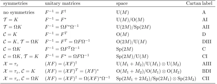
[image:16.595.79.519.529.700.2]

In a specific mathematical sense, it can now be argued that these ten classes provide a complete classification of random-matrix ensembles (Zirnbauer, 1996; Caselle and

Table 2.2 Classification of unitary matrix ensembles

symmetries unitary matrices space Cartan label

no symmetries F−1=F† U(M) A

T =K F−1=F∗ U(M)/O(M) AI

T = ΩK F−1= ΩF∗Ω−1 U(2M)/Sp(2M) AII

C=K F−1=FT O(M) D

C=K,T = ΩK F−1=FT _{= ΩF}_Ω−1 _O(2M_)/U(M₎ _DIII

C= ΩK F−1_{= ΩF}T_Ω−1 _Sp(2M₎ _C

C= ΩK,T =K F−1=F∗= ΩFΩ−1 Sp(2M)/U(M) CI

X =τz (XF) = (XF)† U(M1+M2)/U(M1)⊗U(M2) AIII

X =τz,C=K (XF) = (XF)T = (XF)∗ O(M1+M2)/O(M1)⊗O(M2) BDI

(17)

Magnea, 2004; Zirnbauer, 2011)—they arise from the groups of unitary, orthogonal and symplectic matrices and the associated compact symmetric Riemannian spaces, as classified by Cartan and summarised in Table 2.2. The three Wigner-Dyson classes with unitary, orthogonal and sympletic symmetry (UE, OE and SE) are the labelled A, AI, AII; the corresponding chiral classes (chUE, chOE and chSE) are labelled AIII, BDI, CII; the classes with charge-conjugation symmetryC2_{= 1 and topological} invariants (RE and T-RE) are labelled D and DIII, while the remaining to classes with

C2₌₋_{1 (QE and T-QE) are labelled C and CI.}

2.3 Positive-definite matrices and Wishart-Laguerre ensembles

As we have seen in the construction of the ten Hamiltonian ensembles, it is often useful to study the blocks of a matrix, and compose new matrices out from them. This leads to natural extensions of the ensembles encountered so far, which can be justified via their connection to orthogonal polynomials (Mehta, 2004; Forrester, 2010). From this perspective, the Gaussian hermitian matrix ensembles in the Wigner-Dyson classes are related to Hermite polynomials, while the other ensembles are related to Laguerre polynomials. As mentioned for the chiral symmetry classes, these ensembles are naturally related to positive semidefinite matrices W = X†X, where X is an M0×M-dimensional matrix. It suffices to consider the caseM ≤M0, as otherwise we can simply studyW =XX†.

We again use the symmetry index β = 1,2,4 to distinguish settings where the matrix elementsXlm are real, complex or quaternion. A Gaussian distribution

P(X)∝exp(−c0_βtrX†X) (2.12) then defines the Wishart-Laguerre ensemble for W, where we set c0_β = β/2σ2. This ensemble was first introduced by Wishart (1928) in the context of multivariate statis-tics, which marks the historical beginnings of random-matrix applications. The joint probability density of the eigenvaluesλofW is given by

P({λn})∝ Y

n<m

|λn−λm|β Y

k

λβ(1+M_k 0−M)/2−1exp(−c0_βλk), (2.13)

which relates to the previously encountered eigenvalue distributions by the substitution λn=En2. As mentioned above, the resulting eigenvalue correlations can be expressed in terms of Laguerre polynomials.

For large matrix dimensions the eigenvalue density approaches the Marchenko-Pastur law (Marˇcenko and Pastur, 1967)

ρ(λ) = M T0 2πλ

p

(λ−λ−)(λ+−λ) forλ− < λ < λ+, (2.14)

where λ± = (

√

(18)

Jacobi ensembles 15

2.4 Jacobi ensembles

A third class of classical orthogonal polynomials appearing in random-matrix problems are the Jacobi polynomials. These are associated with joint probability distributions of the form (Forrester, 2010)

P({µn})∝ Y

n<m

|µn−µm|β Y

k

(1−µk)aβ/2(1 +µk)bβ/2, (2.15)

whereµm∈[−1,1],m= 1,2,3, . . . , M.

Such distributions arise, for instance, when one considers the singular values of anM0×M dimensional off-diagonal blocktof a suitableN×N dimensional unitary matrixF(Beenakker, 1997; Beenakker, 2015). In particular, settingN =M+M0with M0 ≥M and generating F from the three standard circular ensembles (COE, CUE or CSE), the eigenvalues Tn = (1−µn)/2∈[0,1] oft†tobey a Jacobi ensemble with a=M0−M+1−2/β,b= 0; similarly, ifF is taken from O(M+M0) or Sp(2M+2M0) (symmetry class D or C) one finds the sameabut b= 1−2/β; the complete picture is presented in Section 4.4.

Alternatively (Forrester, 2010), the quantitiesTncan be interpreted as the eigenval-ues of a so-called MANOVA matrix (X†_X_+Y†_Y₎−1_X†_X_{, where}_X_and_Y _{are matrices} of dimensionsMx×M and My×M, distributed as Gaussians with equal varianceσ according to Eq. (2.12). In this case,a=Mx−M+ 1−2/β,b=My−M + 1−2/β. As shown based on this realization in the Appendix, in the limit of a large matrix dimensionM with fixedcx=Mx/M,cy =My/M the eigenvalue density approaches

ρ(T) = M(cx+cy) p

(T−T−)(T+−T)

2πT(1−T) , (2.16)

where

T±= 1 1 +λ∓

, λ±=

√

cxcy±pcx+cy−1 cx−1

!2

(2.17)

determines the range where the density is finite. In terms of the variables µn, this takes the form

ρ(µ) = M(cx+cy) 2π

p

(µ−µ−)(µ+−µ)

1−µ2 , (2.18)

within the boundaries given byµ±= (λ±−1)/(λ±+ 1).

2.5 Non-hermitian matrices

(19)

vn are not orthogonal to each other, so that the spectral decompositionX=V DV−1 withD= diag(zn) involves a non-unitary matrixV. We therefore need to distinguish the right eigenvectors vn, which form the columns of V, from the left eigenvectors

wn, which are obtained from wnX =snwn. Imposing the biorthogonality condition

wmvn=δnm, the left eigenvectors form the rows ofV−1.

This biorthogonal set of eigenvectors is in general no longer normalised. The extent of mode non-orthogonality can thus be quantified by the condition numbers (Chalker and Mehlig, 1998; Janiket al., 1999; Schomeruset al., 2000)

Omn=

(v†mvn)(wnw†m)

(v†mwm† )(wnvn)

, (2.19)

which we have written in a way that does not rely on the chosen normalisation condi-tion. In terms of the matrixV,

Omn= (V†V)mn(V−1V−1†)nm. (2.20)

The diagonal elements Km = Omm are real and obey Km ≥ 1, with Km = 1 for all m only if V is unitary. These quantities become large in particular when two eigenvalues approach each other closely, and indeed diverge at eigenvalue degeneracies, so-called exceptional points (Berry, 2004; Heiss, 2012). Close to such a degeneracy with a coalescing pairzn+1=zn,Xcannot be diagonalised but only be brought into a form involving Jordan blocks

zn 1

0 zn

. (2.21)

This means that the eigenvectors of the modes become identical, in sharp contrast to hermitian systems where the eigenvectors remain orthogonal as one approaches a degeneracy.

The probability distribution (2.12) for M ×M-dimensional square matrices X defines the Ginibre ensemble (Ginibre, 1965; Khoruzhenko and Sommers, 2011). For the complex Ginibre ensemble (β= 2), the joint distribution of eigenvalues is

P({zn})∝ Y

n<m

|zn−zm|2 Y

k

exp(−c0_βz2_k). (2.22)

In the quaternion case β = 4 eigenvalues come in conjugate pairs, and the joint distribution of eigenvalues in the upper half of the complex plane

P({zn})∝ Y

n<m

|zn−zm|2|zn−z∗m| 2Y

k

|zk−z∗k|

2_exp(₋_c0 βz

2

k) (2.23)

(20)

Non-hermitian matrices 17

for small spacingss=|zn−zm|, where one power ofsarises from the area element in the complex plane.

As shown in the Appendix for the complex Ginibre ensemble, for a variance scaled to σ2 = 1/M and M → ∞ the eigenvalue density in the complex plane approaches Ginibre’s circular law ρ(z) = M_πΘ(1− |z|), where Θ denotes the unit step function. As a side product of the calculation presented there (Janiket al., 1999), the condition number Km|zm=z ∼ M(1− |z|

2_{) turns out to be large, unless one approaches the}

boundaries of the eigenvalue support.

From the general perspective of commutation and anticommutation with unitary and anti-unitary symmetries, non-hermitian matrices admit a very large number of symmetry classes (Magnea, 2008). For a physical setting that illustrates this richness, we can consider photonic systems with absorption and amplification (Cao and Wiersig, 2015). Without further constraints we may model these as a complex Ginibre ensem-ble (β = 2) with different weights of the hermitian and non-hermitian contributions, where the eigenvalue support becomes elliptic (Girko, 1986). Time-reversal symmetry in optics (reciprocity) makes the matrix complex symmetric,H =HT ₆₌_H∗_{, which} modifies the statistics but does not entail any spectral constraints. As a template for the real Ginibre ensemble (β = 1), we can take a system with balanced amplification and absorption, situated in regions that are mapped onto each other by a reflection or inversionP (Makriset al., 2008; R¨uteret al., 2010). We then obtain a non-hermitian PT-symmetric system withP HP =H∗6=HT (Bender, 2007), which in a suitable ba-sis is represented by a real asymmetric matrix. In combination with magneto-optical effects, we can similarly construct PTT0-symmetric systems with P HP = H† 6=H (Schomerus, 2013a). The spectrum remains symmetric about the real axis, and a random-matrix analysis reveals a close connection to the real Ginibre ensemble, in-cluding the same accumulation ofO(√M) eigenvalues on the real axis (Birchall and Schomerus, 2012). Further examples can be constructed by modifying the role ofP. In an optical system where P represents a chiral symmetry, we can realize the case H =−P H∗P in which eigenvalues are symmetric with respect to the imaginary axis (Schomerus and Halpern, 2013; Schomerus, 2013b; Poli et al., 2015), as well as the caseH =H∗=−P HP in which eigenvalues are symmetric with respect to both the real and the imaginary axis (Malzard et al., 2015). For a symmetry with P2 ₌ ₋₁ (hence P =−PT_{, assuming} _P _{is real), two interesting cases are the so-called} Hamil-tonian ensembles withP HP =HT, as well as the skew-Hamiltonian ensembles with P HP =−HT (these notions relate to the symplectic structure of classical Hamiltoni-ans, generated by an antisymmetric involution such asP; Beenakker et al.2013). For a real Hamiltonian matrix with Gaussian statistics,O(√M) eigenvalues accumulate both on the real and on the imaginary axis; for a real skew-Hamiltonian matrix, all eigenvalues are twofold degenerate andO(√M) of these pairs accumulate on the real axis.

(21)

3 The scattering matrix

In this chapter we develop effective models for the scattering matrix and use these to identify the associated random-matrix ensembles.

3.1 Points of interest

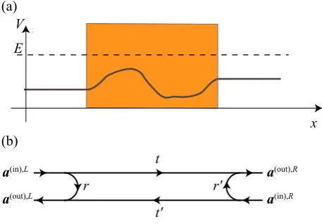
Consider a particle moving through a scattering region with a spatially varying po-tential energy V, as sketched for a simple one-dimensional setting in Fig. 3.1. The corresponding Hamiltonian is ˆH = ˆT+ ˆV, where ˆT represents the kinetic energy. Here are some natural phenomena that we may wish to consider: Decay, where we address the escape rate of a particle inserted into the scattering region; transport, where we address the probability for an incident particle to be transmitted or reflected; dynam-ics, where we ask how long the particle engages with the scattering region and how many internal states it explores. We may also wish to identify system-specific details beyond the fundamental symmetries, such as regarding the role of different scattering

x V

(a)

(b)

E

r

a(in),L

a(out),L

a(out),R

a(in),R

r′ t′

[image:21.595.131.360.474.633.2]

t

(22)

Definition of the scattering matrix 19

subregions or the role of the contacts. All of these questions (and many more) can be addressed with the help of a single object, the scattering matrixS(E).

3.2 Definition of the scattering matrix

To define the scattering matrix (Newton, 2002; Messiah, 2014) we stipulate that the motion outside the scattering region is ballistic. At any energy E, we then have ac-cess to a complete set of propagating scattering states |ψn(in)i in which the particle is approaching the scattering region (incoming channels), and a corresponding set of propagating states |ψ(out)n i where the particle is moving away from the region (out-going channels). These states are taken to be normalised to a unit probability flux through any closed surface surrounding the scattering region. We may also encounter a set of non-propagating (evanescent) states |ψ(ev)m iwhich decay away from the scat-tering region and do not carry any flux. Outside the scatscat-tering region, we then can write a state with a given energy as

|ψi= N X

n=1

a(in)_n |ψ(in)_n i+ N X

n=1

a(out)_n |ψ_n(out)i+X l

a(ev)_l |ψ_m(ev)i, (3.1)

whereN fixes the number of scattering channels. We collect the expansion coefficients into vectorsa(in), a(out)anda(ev).

Inside the scattering region, we may expand the state in terms of any suitable complete set of modes, |ψi= P

mbm|χmi with a coefficient vector b. With help of the stationary Schr¨odinger equation (1.1), the states inside and outside the scatter-ing region are uniquely related. In particular, if we fix a(in) _{then the solution of the} Schr¨odinger equation uniquely fixes a(out)_, _a(ev)_{, and} _b_{, up to effectively decoupled} parts that can be treated as a separate system. These relations must be linear, so that

a(out)=S(E)a(in). (3.2)

This defines the scattering matrix. Flux normalization ensures that for real energies S(E) is unitary, hence S(E) ∈ U(N). Causality ensures that the poles El of S at complex energies are all confined to the lower half of the complex plane, ImEl <0. The number of propagating scattering channels N may change at certain energies, which gives rise to branch cuts in the complex-energy plane.

3.3 Preliminary answers

The scattering matrix addresses the phenomena listed at the beginning of this chapter in the following ways.

(23)

20 The scattering matrix

so that the corresponding intensity |A(t)|2 _{= exp(}₋_tγ

l) decays with rate γl. For a particle prepared in this state att= 0, the Fourier signal

A(ω) = Z ∞

0

A(t)eiωtdt=i[(ω−El0/~) +iγl/2]−1 (3.3)

delivers the resonance-like frequency-resolved signal

|A(ω)|2= 1

(ω−E_l0/~)2+γl2/4

, (3.4)

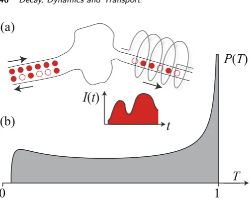
a Lorentzian centred atE_l0/_~ with full width at half maximumγl. When the particle is prepared in a superposition of quasi-bound states, the resulting decay for long times depends on the characteristic decay rateγ0 = infγl, defined such thatγl≥γ0 for all contributing states. If γ0 > 0 the decay becomes exponential, while forγ0 = 0 one typically encounters a power-law.

Transport.—For a particle incoming in channel n, the probability to scatter into the outgoing channel n0 is given by |Sn0_n|2. The unitarity of the scattering matrix

guarantees that the sums of probabilitiesP

n|Sn0_n|2=P_n0|Sn0_n|2= 1 are normalised.

This normalization also holds for an incident particle in any superposition of incoming modes,|a(out)|2₌_|_a(in)_|2_{. These features are at the heart of the scattering approach to} transport (Beenakker, 1997; Blanter and B¨uttiker, 2000; Nazarov and Blanter, 2009). In many settings, we are let to group the scattering amplitudes into subcompo-nentsa(in),s_,_a(out),s_{, where}_s_{labels different asymptotic regions (leads). The scattering} matrix is then formed of blocks Ss0_s describing transmission from lead s to lead s0,

and reflections back into lead sif s0 =s. The associated transmission probability is quantified by the dimensionless conductance gs0_s = tr (S†

s0_sSs0_s). In the case of two

leads, designated as a left lead s=Lwith NL channels and a right lead s=R with NR channels, we write the blocks as

S =

r t0 t r0

, (3.5)

where r andt describe the reflection and transmission of particles arriving from the left, whiler0 andt0 describe these processes for particles arriving from the right. This designation is illustrated in Fig. 3.1(b). The dimensionless conductance is then given byg= trt†t= trt0†t0 =NL−trr†r=NR−trr0†r0, where the stated identities follow from unitarity.

The eigenvaluesTn∈[0,1] of the hermitian matrix t†tare known as the transmis-sion eigenvalues, and determine the dimentransmis-sionless conductance via g =P

nTn. The quantities√Tn can be interpreted as the singular values oft, which generalises to the polar decomposition of the scattering matrix,

S=

V 0 0 V0

√

1−T √T

√

T −√1−T

V00 ₀ 0 V000

, T = diag (Tn) (3.6)

(24)

Preliminary answers 21

The transmission eigenvalues determine many other transport properties, including the full counting statistics of electrons at low temperatures (Levitov and Lesovik, 1993), with the shot noise characterised by the second binomial cumulant (B¨uttiker, 1990; Blanter and B¨uttiker, 2000)

X

n

Tn(1−Tn). (3.7)

Another example is the charge transport through a normal conductor into a con-ventional superconducting lead (Beenakker, 1992; Beenakker, 1997), for which the dimensionless conductance at vanishing magnetic fields is given by

gN S = X

n

T_n2/(2−Tn)2. (3.8)

Dynamics.—Complementing the information about the scattering probabilities, the phaseϕof a scattering amplitudeSn0_n=|S_n0_n|eiϕprovides insight into the dynamics

(de Carvalho and Nussenzveig, 2002; Texier, 2016). For instance, for ballistic propa-gation through a region of lengthLat a constant momentump(E), the particle picks up the dynamical phaseϕ=pL/~. The energy sensitivity~dϕ/dE=L/v=τ of the phase therefore gives an indication of the travel time. In a semiclassical description of scattering from a slowly varying potential, we have ϕ=Scl/~, where the classical actionSclagain obeys dScl/dE=τ.

These observations lead to the formal definition of the delay time of a particle that passes through the scattering region. For injection and extraction in individual chan-nels, the delay time can be isolated by the logarithmic derivative ImS−1_n0_ndSn0_n/dE.

For multi-channel scattering this is generalised by the Wigner-Smith time-delay matrix (Wigner, 1955; Smith, 1960)

Q=−i_~S†dS/dE. (3.9) The unitarity of S at any energy ensures thatQ =Q† is hermitian, while causality ensures thatQis positive semidefinite. Therefore, the eigenvaluesτnofQare real and positive. These eigenvalues are known as the proper delay times.

Noting thatv−1=dp/dE also appears in semiclassical estimates of the accessible phase-space volume, the delay times are intimately related to the density of states. Indeed, the Wigner-Smith matrix directly quantifies the global density of states in the system, in terms of the Birman-Krein formula (Birman and Krein, 1962)

ρ(E) = 1

2π~trQ. (3.10)

Replacing the derivative d/dE by a local variation of the potential ∂/∂V(x), this approach can be extended to obtain the local density of states (Gasparian et al., 1996). Analogous variations with respect to other parameters deliver a wide range of response functions, which can for instance be used to study adiabatic transport and quantum pumping (B¨uttikeret al., 1994; Brouwer, 1998).

(25)

exactly if we extend the scattering matrix to include evanescent states, and often still very reliably if we only account for the propagating states. The simple idea is to in-spect each interface and identify the amplitudes of outgoing states from one region with the amplitudes of incoming states into the adjacent region.

For the case of two adjacent regions with scattering matrices S1, S2 of the form (3.5), the wave-matching of propagating states leads to the composition law

S1⊕2=

r1+t01r2(1−r10r2)−1t1 t01(1−r2r10)−1t02 t2(1−r01r2)−1t1 r02+t2r10(1−r2r01)−1t02

. (3.11)

This rule can be reformulated as a simple matrix multiplicationM =M2M1 for the transfer matrix

M =

t†−1 r0t0−1 r0†t†−1 t0−1

, (3.12)

which relates modes on the left and right according to

aout,R ain,R

=M

ain,L aout,L

. (3.13)

Flux conservation translates to the property M†σzM = σz, so that M is complex symplectic. The eigenvalues ofM†M and (M†M)−1 =σzM†M σz are thus identical and appear in reciprocal pairs, which are given by (p1/Tn±

p

−1 + 1/Tn)2.

We note that in the composed system, according to Eq. (3.11) poles from the multiple scattering across the interface arise from

det[1−r2(E)r01(E)] = 0. (3.14) Similarly, the role of a contact can be studied by inserting a static tunnel barrier at the corresponding boundary of the scattering region (Brouwer, 1995; Beenakker, 1997). For example, the scattering matrix

SB = √

1−Γ2 √_Γ

√

Γ −√1−Γ2

(3.15)

describes a barrier with uniform transparency Γ∈[0,1] in all channels. If we send Γ→

0 for all contacts the system becomes closed. Poles approaching the real axis become the energy levels of the closed system, while poles moving deep into the complex plane are associated with direct reflection processes from the outside.

We can also artificially separate a closed system into two open systems joined by an interface. For a left and a right region, this is described by scattering matrices S1 =r01 andS2=r2, both only composed of a reflection block back to the interface. The quantization condition (3.14) can then be rewritten as

(26)

Effective scattering models 23

t/T

₀

F

P

T

P

Q

F

Q

F

Q

P

T

_P

T

P

n

n+1

[image:26.595.115.355.159.302.2]

n

−1

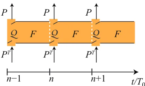
Fig. 3.2 Illustration of the stroboscopic scattering approach, in which particles are injected and collected at regular intervals.

3.4 Effective scattering models

In practice, many methods are available to calculate the scattering matrix in specific settings. This includes wave matching, Green function methods and the boundary integral method, as well as iterative procedures based on the composition rule (3.11) of scattering matrices, and analogous rules for the Green function (Datta, 1997). For the purpose of a statistical description, however, we require a generic model that captures the essential features of the internal dynamics and the coupling to the leads. This is delivered by the Mahaux-Weidenm¨uller formula (Mahaux and Weidenm¨uller, 1969; Livsic, 1973; Verbaarschotet al., 1985; Guhret al., 1998)

S(E) =iπW

†_(E₋_H)−1_W ₋₁

iπW†_(E₋_H)−1_W _{+ 1}, (3.17) whereHis an effective internal Hamiltonian of dimensionM×M whileW is a suitable M×N-dimensional coupling matrix, specified fully in Eq. (3.40).

We provide a motivation of this formula via a detour to the stroboscopic scattering problem (Fyodorov and Sommers, 2000; Tworzyd lo et al., 2003), which leads to its close cousin

S(ε) =KAK T ₋₁

KAKT _{+ 1}, A=

1 +eiε_F 1−eiε_F =−A

†_. _(3.18)

Here F is an effective internal time-evolution operator over a fixed time periodT0,ε is the associated quasi-energy, and the coupling matrixK is fully specified in (3.34). The Mahaux-Weidenm¨uller formula then follows in the continuum limit T0 →0. We present this construction because it gives rather direct intuitive insight into scattering and decay problems, and also helps to isolate and justify the general features of the scattering matrix described in the previous section.

3.4.1 Stroboscopic scattering approach

(27)

Consider a situation where the coupling of the scattering region to the outside occurs stroboscopically, at periodically spaced, discrete times t=nT0≡tn,n= 0,1,2,3, . . . (see Fig. 3.2). Let us denote the state within the system just before these times as

|ψni=|ψ(t−n)i. This state evolves stroboscopically according to

|ψni=FQ|ψn−1i= (FQ)n|ψ0i, (3.19) where F is the unitary operator that describes the time evolution when the system is closed, whileQis a projector that describes what remains in the system when the system is open. In other words, in each time interval, we lose some internal wave amplitude according to the complementary projectorP = 1− Q, while the remaining amplitude is propagated by the unitary time evolution operatorF. As we assume that FandQare independent of the time indexn, we require that the details of the coupling are otherwise time-independent and the internal dynamics are autonomous, or at least themselves time-periodic with period T0. The fact that we take Q as a projector means that the coupling is ballistic—the opening is fully transparent, without any partial reflection of the passing wave. This is also called an ideal lead.

According to Eq. (3.19), the decay of the amplitude within this system is described by the non-unitary operator FQ. In a basis where Q is diagonal this corresponds to truncating the unitary operator F. Let us specify this for a system with a finite internal Hilbert space of dimension M, coupled to N external channels such that rankQ = M −N. In the basis where Q = diag(0,0,0, . . . ,0,1,1, . . . ,1) (N zeros followed byM−N ones),FQis then obtained fromF by setting the firstN columns to zero.

In this setting, the quasibound states|φmiare obtained from the eigenvalue prob-lem

FQ|φmi=zm|φmi, = 1,2, . . . , M. (3.20) Due to the projective nature of Q, there will by N vanishing eigenvalues, while the remaining eigenvalues are in general complex and finite, with|zm|<1. Each eigenvalue describes the exponential stroboscopic decay of the associated quasibound state—if the initial state is|ψ0i=|φmi, the intensity within the system decays as

hψn|ψni=|zm|2nhψ0|ψ0i. (3.21) Writingzm = exp[−i(εm−iγm/2)], the decay constant over a period T0 is given by γm. As indicated, this decay constant is best viewed as arising from the imaginary part of a complex quasienergyε?

m=εm−iγm/2, where the real part is defined modulo 2π. Stroboscopic scattering with ideal contacts. We now turn the stroboscopic decay problem into a stroboscopic scattering problem. This requires to define how the escape from the system translates into particles detected outside, as well as how to feed particles into the system. In other words, we need to define objects that connect the state within the system (residing in the internal Hilbert space in which F and

(28)

In the case of ballistic coupling that we study thus far, the outgoing state can be taken of the simple form

|ψ(out)_n i=P|ψni, (3.22) withP such thatP=PTP = 1− Qrecovers the rank-N projector that complements

Qin the internal Hilbert space. It follows thatP PT = 1 is the identity in the space of the external scattering channels (the rank does not change under the reordering and the resulting object is still a projector). Recall that the internal state refers to the instance just before we open the system. Therefore, the incoming particle injected in the previous step modifies this state according to

|ψni=FQ|ψn−1i+F PT|ψn−1(in)i = (FQ)n|ψ0i+

n−1 X

l=0

(FQ)lF PT|ψ_n−l−1(in) i, (3.23)

which replaces Eq. (3.19). Combining these expressions, we find

|ψ(out)n i=P(FQ) n

|ψ0i+P n−1 X

l=0

(FQ)lF PT|ψ(in)_n−l−1i. (3.24)

The first part recovers the decay of the initial state, while the remaining part describes the scattering. The pure decay problem is characterised by the absence of the incoming state, while the pure scattering problem is characterised by the absence of the initial state.

Both these problems now turn out to be intimately related. For this, we revert back to a continuous time variable,|ψ(out)_(t)_i₌P

nδ(t−nT0)|ψ (out)

n i, and perform a Fourier decomposition of the scattered signal,

|ψ(out)(ε)i= ∞ X

n=0

eiεn|ψ(out)_n i (3.25)

= ∞ X

l=0 ∞ X

n=l+1

eiεlP(FQ)leiεF PTeiε(n−l−1)|ψ(in)_n−l−1i, (3.26)

hence

|ψ(out)(ε)i=S(ε)|ψ(in)(ε)i (3.27) with the stroboscopic scattering matrix

S(ε) =P ∞ X

l=0

[eiεFQ]leiεF PT =P 1 1−eiε_F_Qe

iε_{F P}T_. _(3.28)

We now observe that the poles of the scattering matrix coincide with the complex quasienergiesε?

(29)

It is convenient to bring the scattering matrix (3.28) into the equivalent form

S(ε) = PAP T ₋₁

PAPT _{+ 1}, A=

1 +eiεF 1−eiε_F =−A

†_. _(3.29)

We then see that the scattering matrix is indeed unitary. Furthermore, this expression nicely generalises to the case of non-ideal contacts, which we address next.

Stroboscopic scattering with non-ideal contacts. To account for non-ideal coupling we insert an energy-independent scatterer at the place of the contact. The contact can be viewed as a region withN channels coupled to the outside andN channels coupled to the inside, and thus is described by a 2N ×2N-dimensional unitary scattering matrix

SB =

rB t0B tB r0B

. (3.30)

The blocks rB and rB0 describe the partial reflection in the external and internal channels, whiletB and t0B describe the transmission into and out of the system. This matrix is assumed to be energy-independent, meaning that the reflection and trans-mission processes from the contact are instantaneous. The return of the particle to the contact is described by the ballistic scattering matrixS0.

We can now match the waves at the contact according to Eq. (3.11), which results in the total scattering matrix

S=rB+t0BS0(1−r0BS0)−1tB. (3.31) This expression has a simple interpretation: The incident wave is either directly re-flected according torB, or enters into the system according totB. Once in the system, the wave undergoes a sequence of l events, each consisting of an internal scattering round tripS0 followed by a partial reflectionrB0 , until after another return S0 to the contact it escapes according tot0_B. Equation (3.31) follows by summing overl, which is of the form of a geometric series.

Inserting forS0the stroboscopic scattering matrix (3.28) for ideal contacts, we find that this can be written more directly as

S=rB+t0BP

1 1−eiε_F(_Q₊_PT_r0

BP)

eiεF PTtB. (3.32)

To further simplify this expression we choose an appropriate basis for the internal state, as well as for the incoming and the outgoing state. This follows from the polar decomposition (3.6), which we need to adopt in the slightly more general form

SB =

V 0 0 V0

−Σ√1−Γ2 √_Γ

√

Γ Σ√1−Γ2

V00 0 0 V000

,

Γ = diag (Γn) Σ = diag (σn)

.

(30)

and real. Starting from (3.32), this basis choice results in the desired generalization of Eq. (3.29),

S= KAK T ₋₁

KAKT _{+ 1}, A=

1 +eiε_F 1−eiε_F =−A

†_, _K_{= diag (κ}σn

n )P, (3.34)

where the contact is now characterized by the coupling coefficients

κn= Γ−1/2n (1− p

1−Γ2

n). (3.35)

These coefficients take the valueκn = 1 for Γn= 1 and κn ≈

√

Γn/2 for Γn1. As they enter the matrixK to the powerσn, a semitransparent contact can be achieved both by decreasing the coupling (σn = 1) or by increasing the coupling (σn =−1). This completes the derivation of the stroboscopic scattering matrix (3.18).

3.4.2 Continuous-time scattering theory

To realize the time-continuous limit of the stroboscopic scattering theory, we setε= ET0/~,F = exp(−iT0H/~), and equateT0≡2π~/M∆ =TH/M to the dwell time in a continuous system withM channels and mean level spacing ∆ (this is the mean time for a round tripF in the system). In the leading orders ofT0, we can approximate

eiεF ≈ 1−iT0(H−E)/2~

1 +iT0(H−E)/2~

, (3.36)

so that

A= 1 +e iε_F

1−eiε_F ≈ 2i_~

T0

G(E), G(E) = 1

E−H, (3.37) where G(E) is the Green function (or resolvent) of the closed system. For the ideal case with scattering matrix (3.29), we then have

S = 2i~

T0P(E−H)

−1_PT ₋₁ 2i~

T0P(E−H)

−1_PT _{+ 1}, (3.38)

while for non-ideal leadsP is replaced byK. InsertingT0completes the derivation of the Mahaux-Weidenm¨uller formula (3.17),

S(E) = iπW

†_(E₋_H)−1_W ₋₁

iπW†_(E₋_H)−1_W _{+ 1}, W =

√

M∆ π K

†_, _(3.39)

where theM×M-dimensional hermitian matrixH represents the Hamiltonian of the closed systems, while theM×N-dimensional matrixW describes the coupling to the N scattering channels. With our basis choice,W is diagonal, with elements

Wnn=

√

M∆ π κ

σn

n (3.40)

(31)

E

−E

X

T

C

a

a*

[image:31.595.113.357.156.274.2]

a*

Fig. 3.3 Fundamental symmetries relate various states of motion, which constrains the scat-tering matrix in accordance to the ten universality classes for unitary matrix.

Equation (3.39) can be rewritten in the equivalent form

S(E) =−1 + 2πiW†(E−H+iπW W†)−1W. (3.41) According to this, the poles of the scattering matrix are given by the eigenvalues of the effective non-hermitian Hamiltonian H−iπW W†_{. The poles all lie in the lower} half of the complex plane, as required by causality. Furthermore, the Wigner-Smith time-delay matrixQ=−i_~S†dS/dE takes the form

Q= 2π~W†(E−H−iπW W†)−1(E−H+iπW W†)−1W, (3.42) which is explicitly positive semidefinite, as again required by causality.

3.5 Merits

Via the stroboscopic model (3.34), the orthogonal, unitary, or symplectic symmetry ofF in the three Wigner-Dyson classes with different form of time-reversal symmetry translates directly into a corresponding symmetry of S. Via the continuous model (3.41), one finds that this also agrees with the corresponding symmetry class forH. In the symmetry classes with chiral or charge-conjugation symmetry, this translation holds when the scattering matrix is evaluated at the spectral symmetry pointsE= 0 or ε = 0, π (away from these points, the symmetry reduces to the three Wigner-Dyson classes). Thus, the ten symmetry classes listed in Table 2.2 directly apply to the scattering matrix, with energy fixed to the symmetry point where required (Beenakker, 2015).

It is instructive to verify these statements directly within the scattering picture (see Fig. 3.3). For this, consider that the time-reversal operation T transforms incoming modes into outgoing modes. If this is a symmetry of the Hamiltonian then the corre-spondingly transformed scattering state must be described by the original scattering matrix. ForT =K this delivers

a(in)∗=S(E)a(out)∗=S(E)S∗(E)a(in)∗, (3.43)

Random matrix approaches to open quantum systems