doi:10.4236/jbise.2010.39114 Published Online September 2010 (http://www.SciRP.org/journal/jbise/).
Comparison of computation time for estimation of dominant
frequency of atrial electrograms:
Fast fourier transform, blackman tukey, autoregressive
and multiple signal classification
Anita Ahmad1, 3, Fernando Soares Schlindwein1, Ghulam André Ng2
1
Department of Engineering, University of Leicester, Leicester, UK; 2
Leicester NIHR Biomedical Research Unit in Cardiovascular Disease, Glenfield Hospital, Leicester, UK; 3
B Faculty of Electrical Engineering, Universiti Teknologi Malaysia, 81310 Johor Bahru, Johor, Malaysia. Email: [email protected]; [email protected]; [email protected]
Received 28 April 2010; revised 1 June 2010; accepted 8 June 2010.
ABSTRACT
Dominant frequency (DF) of electrophysiological da- ta is an effective approach to estimate the activation rate during Atrial Fibrillation (AF) and it is import- ant to understand the pathophysiology of AF and to help select candidate sites for ablation. Frequency analysis is used to find and track DF. It is important to minimize the catheter insertion time in the atria as it contributes to the risk for the patients during this procedure, so DF estimation needs to be obtained as quickly as possible. A comparison of computation tim- es taken for spectrum estimation analysis is present- ed in this paper. Fast Fourier Transform (FFT), Bla- ckman-Tukey (BT), Autoregressive (AR) and Multi-ple Signal Classification (MUSIC) methods are used to obtain the frequency spectrum of the signals. The time to produce DF was measured for each method. The method which takes the shortest time for analysis is selected for real time application purpose.
Keywords: Fast Fourier Transform; Blackman-Tukey; Autoregressive; MUSIC; Frequency Analysis
1. INTRODUCTION
During AF, atrial electrical activity is described as chao- tic and random [1]. Frequency domain analysis can help to interpret such activity. DF analysis has been used in several fields such as acoustic emission [2], speech perc- eption [3] and cardiac arrhythmias [4]. DF is defined as the frequency of the signal at the point where the frequ- ency spectrum has the maximum value.
The current available treatment of AF consists of me- dication, electrical cardioversion and ablation. Typically,
antiarrhythmic medications such as amiodarone, propa- fenone and flecainide are used for sinus rhythm control [5] but they are not effective to prevent irregular rhyt- hms.
If medication is not suitable to control the sinus rhy- thms, electrical cardioversion is considered [6]. The pro- cedure is called defibrillation. It can be performed in 2 different ways: at the hospital (electrical cardioversion) or using an implantable cardioverter-defibrillator device (ICD).
When medication and electrical cardioversion control fail, ablation is usually the next step to be considered. Catheter-based radio frequency ablation therapies offer a chance to cure AF. The chances for people survival were 98% and 95% in year 1 and year 2 respectively [5]. The ablation performed in early paroxysmal AF has the hig- hest chance for success compared to its use for persistent and permanent AF [7]. The success rate of ablation at DF site is shown by significant prolongation of the atrial fibrillation cycle length (AFCL) compared to the site with non-dominant frequency [8,9]. This result supports the use of DF mapping to identify suitable ablation tar-gets.
Catheter ablation of AF is a complex interventional el- ectrophysiologic procedure. Its risk is higher than that of ablation for other cardiac arrhythmias [10]. The worldw- ide survey of AF ablation reported that 6.0% complica-tion was recorded (524/8745) [11]. Univariate analysis stated that sex, age, insertion difficulty, length of the ins- erted catheter, type of catheter and, term of insertion were among contributors for catheter related blood stream in- fection [12]. The risks include requiring prolonged hos-pitalization, long-term disability or death [13].
proce-dure is one of the contributors to blood stream infection, computation time is critical for any technique to be used during any surgical procedure. Shortening the analysis time can significantly influence the risk of overall surgi-cal procedure. Our aim in this study is to compare the computation time for four different spectrum analysis techniques and compare the different techniques in their ability for producing accurate results.
With current technology the data collection capability for non-contact mapping systems consists of catheter mo- unted multielectrode array allowing the recording up to 3000 points of virtual electrophysiological data at 1200 Hz. With this number of data points, it is important to identify an approach that could be used to produce DF with minimum computation time.
This will in turn help electrophysiologist to identify the dangerous frequencies as target ablation sites and to apply ablation effectively in an expeditious manner. Frequencies between 6-15 Hz are classified as ‘danger-ous’ as the atria fires in an irregular and chaotic fashion. The main objective of this study is to reduce the risk during catheter procedure by selecting the technique for estimation of DF with the shortest computation.
2. FREQUENCY DOMAIN ANALYSIS
2.1. Fast Fourier Transform (FFT) Technique
The application of the Fast Fourier Transform (FFT) is important in signal processing computations using speci- ally in spectral analysis [13]. The discrete Fourier trans-form of x nT
is given by
1
0
2 N
n k
X x nT e
NT N
j nk
(1)The FFT algorithm is the main choice for obtaining the Discrete Fourier Transform (DFT) because of its sp- eed.
Welch technique based on FFT algorithm is used to co- mpute the periodogram. This technique uses signal seg-mentation and averaging to improve statistical properties of the spectral estimates [14]. The equation for comput-ing the averaged periodogram is:
1
1
ˆ M ˆ 0 2
w k m k k s
m
P f P f f f
m
(2)where is the periodogram of the mthsegment of data.
ˆm k
P f
The ends of the data sequence are tapered to zero wh- en data is windowed. DF was obtained from the Welch/ FFT analysis. There are a few considerations to the use of DF analysis especially for the electrograms [4]:
a) The estimation of the power spectrum uses the FFT because this is an efficient and widely available method.
b) The maximum frequency is inversely proportional
to the sampling interval t as t
2
1 .
The frequency resolution in the power spectrum is inv- ersely proportional to the length of the signal
T f 1
where T is the length of the signal collected
T N t
. This has implications for the interpretation of the DF obtained.2.2. Blackman-Tukey (BT) Technique
This method was proposed by Blackman and Tukey (1958) [13]. The estimator is based on the Wiener-Kh- inchin theorem, which states that the power spectrum density is the Fourier Transform of the autocorrelation function of the series [15,16].
If fewer data points are used, the variance of the aut- ocorrelation estimate increases and the estimate become less reliable [13]. The averaging associated with win-dowing a series decreases the resolution of the method, from the frequency intervals of 1/N, to a windowed fre-quency interval of about 1/M, where M is the length of the window. As a result, wider windows yield higher sp- ectral resolution, and vice versa. The drawbacks of Bla- ckman-Tukey are suppression of weak signal main-lobe responses by strong signal sidelobe and frequency reso-lution limited by the available data record duration.
This method involves 3 steps [13]:
1) The autocorrelation sequence of the data is esti-mated using the formula;
10
1
ˆ N 0,1, 2, 1
xx n n m
n
R m x x m N
N
(3)where: xn is the n-th value of the data series, N is the
total number of points in the data series m is the auto-correlation lag ^ signifies estimated value.
2) Windowing the autocorrelation sequence.
The windowing of the autocorrelation sequence is no- rmally carried out using a hamming window that has the following characteristics:
2
0.54 0.46 cos , 1 1
0,
m
w m M m M
M w m otherwise
(4)
3) Finding the Fourier transform to yield the following PSD estimate [15]:
1
2
1
ˆ M ˆ j fm
BT xx
m M
P f R m w m e
(5)where: w (m) is a window function of length 2(M-1)-1, which is zero for |m| M-1
The PSD estimate is determined over the frequency
range 1 1
2fs f 2fs
fre-quency.
2.3. Autoregressive (AR) Technique
Autoregressive technique involves selection of model or- der and the estimation of model parameters from the co- llected data. This technique is widely used because it has a rational transfer function and the algorithm to estimate the parameters results in a system of linear equations [15]. In this model, the data xn are considered to be the
output of a system with a random input un. The relation
between input and output are described by the following difference equation which represents the auto-regressive moving average ARMA (pole-zero) model:
1 0
p q
n pk n k qk n k
k k
x a x b u
(6)where: p,q are model orders for the AR and the MA pa- rts, respectively a,b are model parameter (apk being the
kth parameter of the pth-order model)
The autoregressive (AR) part of this general equation is given by:
1
p
n pk n k
k
n
x a x u
(7)Knowing p past values of the series we can estimate the next output as:
1
ˆ p
n pk
k
n k
x a x
(8)Equation (8) defines the AR with all-pole model. Wh- ile, the MA model is given by:
0
ˆn qk qk n k
x
a u (9) The prediction error epn is defined as the differencebetween the actual sample value xn and its predicted
value ˆxn.
1
ˆ
p
pn n n n pk n k
k
e x x x a x
(10)The power spectrum of an AR process is:
2 22 1 ˆ
1
e AR
p j fk
pk k
P f
a e
(11)where 2
e
is the variance of epn.
2.4. Multiple Signal Classification (MUSIC)
The multiple signal classification is the improvement of Pisarenko harmonic decomposition [17]. This is an ei-gen-based subspace decomposition method and is best used to estimate the frequencies of complex sinusoids in additive white noise [18].
Assume that y(n) is a random process that consists of
p complex exponentials in white noise,
2
1
k k p
j f n k k
y n A e n n
(12)The autocorrelation matrix of a noisy signal can be written as:
yy xx n
R R Rn (13)
where: xx is the autocorrelation matrix of the signal
is the autocorrelation matrix of the noise.
R
nn
R
Eigen-analysis is used to partition the eigenvectors and the eigenvalues of the autocorrelation matrix of a noisy signal into 2 subspaces, signal subspace and noise subspace. The eigenvector can be divided by two groups, the p signal eigenvector corresponding to the p largest eigenvalues and M – p noise eigenvector corresponding to the smallest eigenvalues [19].
Ideally, p of these roots will lie in the unit circle on the frequencies of the complex exponentials. The small-est eigenvalue determines the noise variance and the corresponding eigenvector is the prediction polynomial for the clean signal [20].
In MUSIC, the effects of spurious peaks are reduced by averaging. The power spectrum estimate is defined as
21
N H
xx k
k p
P f v e f
(14)where N is the dimension of the eigenvectors vk is the
k-th eigenvector of the correlation matrix p is the dimen-sion of the signal subspace.
Since Pxx
f has its zeros at the frequencies of the sinusoids, hence the reciprocal of Pxx
f has its poles at these frequencies [18]. Then, the MUSIC spectrum can be written as
2 11
MUSIC N
H k k p
P f
v e f
(15)3. METHOD
The spectrum estimation analysis was tested using sinu-soid signals in noise to identify their DF using the 4 dif-ferent approaches. In FFT analysis, Welch method esti-mates the frequency spectrum of the signals. The Fourier transform was calculated separately for each of the seg-ments. The analysis was performed by taking the aver-age of the segments, each with 2048 points, using a 4096-point FFT and an overlap of 50% with a hamming window.
In Blackman-Tukey method, the autocorrelation was determined using 4096 points. This autocorrelation func-tion was windowed with the same hamming window used for the FFT approach (4096-point).
the finite linear aggregate of the previous value of the process and the current value of white noise. The model order used was p = 8.
As for MUSIC, two complex exponentials with the same window are used to identify the spectrum.
4. RESULTS
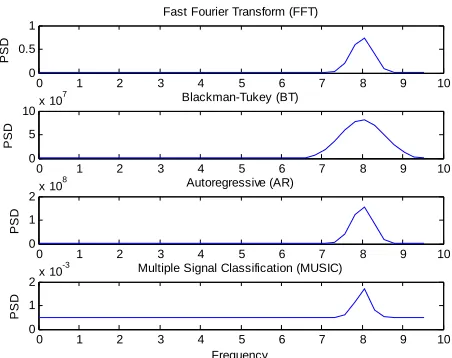
[image:4.595.58.284.316.495.2]The spectrum estimation was determined using several test frequencies: 8.0 Hz, 7.7 Hz, 7.0 Hz, 6.3 Hz, 5.5 Hz and 5.0 Hz. Figure 1 shows the graphical results of FFT, Blackman-Tukey, Autoregressive and MUSIC in which tested using sinusoidal wave of 8 Hz. DF is being con-sistently estimated as 8Hz.
Table 1 shows the DF value comparison for all tech-niques against the base Frequency.
The results show consistent value of DF produced by all techniques.
Table 2 shows that, the percentage error is of the same order of magnitude for these 4 techniques.
0 1 2 3 4 5 6 7 8 9 10
0 0.5 1
Fast Fourier Transform (FFT)
PS
D
0 1 2 3 4 5 6 7 8 9 10
0 5 10x 10
7 Blackman-Tukey (BT)
PS
D
0 1 2 3 4 5 6 7 8 9 10
0 1 2x 10
8 Autoregressive (AR)
PS
D
0 1 2 3 4 5 6 7 8 9 10
0 1 2x 10
-3 Multiple Signal Classification (MUSIC)
Frequency
PS
D
[image:4.595.56.282.579.636.2]Figure 1. Comparison of Fast Fourier Transform, Blackman- Tukey, Autoregressive and Multiple Signal Classification spec-tral estimates.
Table 1. DF value comparison for all technique against the ba- se Frequency.
Base
Frequency(Hz) 8 7.7 7 6.3 5.5 5
Frequency
Estimation(Hz) 8.06 7.81 7.08 6.35 5.62 4.88
Table 2. Calculation of error for FFT, Blackman-Tukey, Autore- gressive and Multiple Signal Classification spectral estimates.
Frequency 8 7.7 7 6.3 5.5 5
% error 0.71 1.47 1.14 0.76 2.09 2.34
Table 3. Computation time for 3000 signals.
Time calculated in seconds for 3000 signals Frequency
FFT BT AR MUSIC
Average 22.8 340.9 206.4 10851.8
For calculation purpose we are using 3000 data series to calculate total computation time. As mentioned before 3000 points is the state-of-art for mapping atrial activa-tion.
Table 3 shows a significant difference in processing time between the 4 techniques tested. In summary, FFT takes 22.8 seconds to process 3000 signals compared to 340.9 s for BT, 206.4 s for AR and 10851.8 s for MUSIC. As discussed before, all techniques produce the same estimation for DF. Therefore, the time taken to produce the estimation is the main factor for the choice of which technique should be used.
5. CONCLUSIONS
The study shows significant difference in computation time between the techniques while the estimated value for DF was the same for all four techniques. The choice of a particular technique contributes to the overall surgi-cal procedure time. As discussed before the duration of catheter deployment is a factor that can contribute to blood stream infection. Therefore, the selection of the fastest technique will reduce the risk of the procedure.
As shown by the result of this study, FFT is the best technique as it produces accurate estimates of DF in a speed compatible for quasi real-time analysis.
6. ACKNOWLEDGEMENTS
This study (or the work described in this paper) is part of the research portfolio supported by the Leicester NIHR Biomedical Research Unit in Cardiovascular Disease.
REFERENCES
[1] Ng, J., Goldberger, J. J. (2007) Understanding and inter-preting dominant frequency analysis of AF electrograms, Journal of Cardiovasc. Electrophysiol, 18(6), 680-685. [2] Woo, S.-C. and Goo, N.-S. (2007) Analysis of the
bend-ing fracture process for piezoelectric composite actuators using dominant frequency bands by acoustic emission.
Composites Science and Technology,67, 1499-1508. [3] Lindblom Björn, Diehl Randy and Creeger Carl.(2009)
Do ‘Dominant Frequencies’ explain the listener’s re-sponse to formant and spectrum shape variations? Speech Communication, 51(7), 622-629.
omini, G., Mazzone, P., Gulletta, S., Gugliotta, F., Papp- one, A. and Santinelli, V. (2003) Mortality, morbidity, and quality of life after circumferential pulmonary vein ablation for atrial fibrillation: Outcomes from a control- ed nonrandomized long term study. Journal of American college of cardiology, 42(2), 185-197.
[6] Jacquemet, V., Kappenberger, L. and Henriquez, C. S, (2008) Modeling atrial arrhythmias: Impact on clinical diagnosis and therapies. IEEE Reviews in Biomedical Engineering,1,94-144.
[7] Gonska, B.D., Bauerle, H.J.and Japha, T. (2009)Atrial fibrillation ablation: Who comes into consideration? Her-
zschrittmachertherapie und Elektrophysiologie, 20(2), 76-81.
[8] Skanes, A.C., Mandapati, R., Berenfeld, O., Davidenko, J.M. and Jalife J. (1998) Spatiotemporal periodicity dur-ing atrial fibrillation in the isolated sheep heart. Circula-tion, 98(12), 1236-1248.
[9] Mandapati, R., Skanes, A., Chen, J., Berenfeld, O. and Jalife, J. (2000) Stable microreentrant sources as a me- chanism of atrial fibrillation in the isolated sheep heart.
Circulation, 101(2), 194-199.
[10] Calkins, H., Brugada, J., Packer, D.L., Cappato, R., Chen, S.A. and Crijns, H.J. et al (2007). HRS/EHRA/ECAS expert consensus statement on catheter and surgical abla-tion of atrial fibrillaabla-tion: Recommendaabla-tions for personnel, policy, procedures and follow-up. Europace, 9(6), 335- 379.
[11] Cappato, R., Calkins, H., Chen, S.A., Davies, W., Iesaka, Y., Kalman, J., Kim, Y.H, Klein, G., Packer, D. and Ska- nes, A. (2005) Worldwide survey on the methods, effi-cacy, and safety of catheter ablation for human atrial
fib-rillation. Circulation, 111(9), 1100-1105.
[12] Prudente, L.A., Moorman, J.R., Lake, D., Xiao, Y., Greebaum, H., Mangrum, J.M., Dimarco, J.P. and Fer-guson, J.D. (2009) Femoral vascular complications fol-lowing catheter ablation of atrial fibrillation. Journal of Interventional Cardiac Electrophysiology,26(1), 59-64. [13] Ifeachor Emmanuel, C. and Jervis Barrie, W. (2002)
Digital signal processing:A practical approach. 2nd Edi-tion, Prentice Hall, New Jersey.
[14] Welch Peter, D. (1967) The use of fast fourier transform for the estimation of power spectra: A method based on time averaging over short, modified periodograms. IEEE Transcations on Audio and Electroacoustics, 15(2), 70- 73.
[15] Kay Steven, M. (1988) Modern spectral estimation the-ory & application. Prentice Hall, New Jersey.
[16] Beauchamp, K. and Yuen C. (1979) Digital methods for signal analysis. George Allen & Unwin, London. [17] Schmidt R. (1979) Multiple emitter location and signal
parameter estimation. Proceedings of RADC spectrum estimation workshop, Saxpy Computer Corporation, USA, 243-258.
[18] Vaseghi Saeed, V. (2008) Advanced digital signal proc-essing and noise reduction. 3rd Edition, Wiley, Chiches-ter.
[19] Hayes Monson, H. (1996) Statistical digital signal proc-essing and modeling. John Wiley & Son, Chichester. [20] Pisarenko, V.F. (1973) The retrieval of harmonics from a