University of Twente
EEMCS / Electrical Engineering
Control Engineering
Learning Multi-Agent Control
with OROCOS
Iker Rezola
MSc report
Supervisors Prof.dr.ir. A. van Amerongen
dr.ir. T.J.A. de Vries MSc P.B. Dao January 2009 Report nr. 001CE2009 Control Engineering
EE-Math-CS University of Twente
Summary
The title of the Master Thesis that the reader has obtained is Learning Multi-Agent Control with Orocos. The compact and accurate name shows perfectly the topics this thesis deals with. The thesis title can be splitted in three parts. The main goal of this thesis has been focussing on these with this three groups.
1 Learning: During the last years, new control techniques have been developed around the world. The traditional feedback controller is still one of the best known. However, feedback controllers can have some faults, to defeat some of those faults a learning feedforward con-troller (LFFC) has been used. The use of feedforward concon-trollers is becoming common in the last years, the research done in this type of controllers is leading to better ways of con-trol. Instead of using a "simple" feedforward controller, a learning feedforward controller has been used in this project. This way of controlling is being analyzed and developed in some universities, the purpose is to improve results while the system keeps on working.
2 Multi-Agent Systems: MAS are also being analyzed and developed . Dividing a complex prob-lem into smaller ones to achieve the main goal is something that has been done since the begining of the human race. The last years it has been proven that this way of working is really useful in computer science, and it has lead towards the most efficient algorithms, such as quicksort or FFT. This way of working has been named divide and conquer algorithms. During the thesis different agents have been described to obtain a wanted behaviour of the plant.
3 OROCOS: Different software applications could be used to implement LFFC and Multi-Agent system. The chosen one has been Orocos. Orocos is an open source-free code project. This software is being developed in a cooperation of different universites. Orocos is a powerful project that in the present and future will continue developing and looking for a open control engineering software.
In this report, these three subjects are explained in more detail and experiences obtained while working with them are documented.
Contents
Summary iii
Contents iv
1 Introduction 1
1.1 Background . . . 1
1.2 Problem definition . . . 1
1.3 Objective . . . 1
1.4 Outline Thesis . . . 1
2 Agents and Multi-Agent Systems 3 2.1 Introduction . . . 3
2.2 Definition . . . 3
2.3 Advantages and disadvantages of using a Multi-Agent System . . . 4
3 Orocos 5 3.1 Introduction . . . 5
3.2 Configuring Orocos . . . 5
3.3 Components . . . 7
3.3.1 Definition . . . 7
3.3.2 Programming components . . . 8
3.3.3 Class . . . 8
Method . . . 9
Data Ports . . . 9
Hooks . . . 10
3.4 Reporting data . . . 11
3.4.1 Configuration . . . 11
3.5 Main program . . . 12
3.5.1 Connect components . . . 12
3.5.2 (A)Periodic activities . . . 13
3.5.3 Reporting Start . . . 14
3.5.4 Start components . . . 14
3.5.5 Stop components and cleaning up . . . 14
4 DemoLin 15 4.1 Introduction . . . 15
5 Feedback controller 17
5.1 PID controller . . . 17
5.2 Block Diagram . . . 18
5.3 Tuning Controller . . . 18
5.4 Low-pass filter . . . 19
5.5 Set point . . . 19
5.6 Discrete system . . . 22
5.6.1 Discretization . . . 22
5.6.2 Discrete plant . . . 22
5.6.3 Discrete controller . . . 23
5.6.4 Actuator and sensor . . . 24
5.7 Implementation in Orocos . . . 24
5.8 Simulation results . . . 25
6 Learning Feed-Forward controller 29 6.1 Introduction . . . 29
6.2 LFFC using B-spline Neural Networks . . . 29
6.2.1 LFFC structures . . . 29
6.2.2 LFFC learning . . . 31
6.3 Programming the B-spline: GSL libraries . . . 33
6.4 Implementation in Orocos . . . 33
6.5 Learning Signal . . . 37
6.6 Learning Component, periodic or non-periodic . . . 37
6.7 Results . . . 38
7 Conclusions 47
8 Future works 49
A Appendix - DemoLin 51
B Appendix - PD controller calculation 53
C Appendix - Used system 57
D Appendix - Codes 59
Bibliography 61
List of Figures
3.1 Orocos Logo. . . 5
3.2 Code::Blocks enviroment settings . . . 6
3.3 Code::Blocks project tree . . . 6
3.4 Port Bifurcation. . . 13
3.5 Non port Bifurcation. . . 13
4.1 DemoLin photo . . . 15
4.2 Model of DemoLin. . . 16
5.1 Parallel PID block diagram. . . 17
5.2 Continuous block diagram . . . 18
5.3 Comparisson among different analog filters. . . 19
5.4 Frequency response of the controller. . . 20
5.5 Open loop system frequency response. . . 20
5.6 Applied reference to the system. . . 21
5.7 Applied acceleration setpoint to the system. . . 21
5.8 Discrete block diagram. . . 22
5.9 Continuous root locus diagram of the open loop system, including: controller, filter, actuator and plant. . . 23
5.10 Connection Map of the feedback controller. . . 24
5.11 Setpoint and output comparisson in the simulated system. . . 25
5.12 Error of the simulated system. . . 26
5.13 Control Signal of the simulated system. . . 26
5.14 RMSD between simulated outputs. . . 27
6.1 Time Index block diagram . . . 29
6.2 A linear process with a non-linearity . . . 30
6.3 State Index block diagram . . . 31
6.4 1st order B-spline . . . 32
6.5 2ndorder B-spline . . . 32
6.6 3r dorder B-spline . . . 32
6.7 Mapping example . . . 33
6.8 Feed-Forward connection map. . . 36
6.9 LFFC control diagram . . . 37
6.10 Error of the system with different amount of data to fit . . . 39
6.11 Error of the system with different order B-splines . . . 40
6.13 Error of the system using a feedback controller. Set point is periodic every 6s.
Mass is changing. . . 43
6.14 Error of the system using a LFFC controller. Set point is periodic every 6s. Mass is changing. . . 44
6.15 Feedback and feed-forward control signals comparisson using a LFFC and a pe-riodic setpoint of 6s. Mass is changing. . . 45
A.1 Schematic diagram of DemoLin . . . 51
B.1 PID block diagram . . . 53
B.2 PD controller frequency response . . . 54
B.3 Frequency response of the open-loop system, havingKc·G(s)·H(s) . . . 54
1 Introduction
1.1 Background
The creator of this thesis landed in The Netherlands on the 1st September of 2008. The MSc project that has been carried out would be a link between previous research projects that were developed at the University of Twente. These research projects are pointing to a number of different techniques or methods that are applicable in advanced control of mechatronic sys-tems. Different projects have been done in the last years in the University of Twente but, for this thesis, it has been focused on two groups:
1 Learning Feedforward Control: LFFC controllers have been developed in the University of Twente since 2000 (22). Different PhD theses have concluded (6, 5) that this type of con-troller is a good way of controlling mechatronic systems.
2 Multi-Agent Control Systems: MAS is also a relatively new concept in control engineering (2001) (21). Since van Breemen wrote his thesis several master theses and individual assig-ments have continued developing the topic of Multi-Agent Control System (9, 10, 3).
Nevertheless, no projects have been done before in the University of Twente using OROCOS as a control framework.
1.2 Problem definition
The first step towards solving a problem is defining the problem. This report tries to explain how to solve the next problem:
Integrate LFFC, Multi-Agent methods and a modern implementation framework (Orocos) so as to obtain a suitable framework for advanced control of mechatronic systems.
Multi-Agent Control Systems have to become Tasks in Orocos, and LFFC as a pattern for in-corporation in a Multi-Agent Control System, with the specific property that learning is done asynchronously, in a separate non-realtime Task.
1.3 Objective
Goal of the project is to evaluate the feasibility of the proposed integration. This is to be done by designing and implementing a simple Multi-Agent Control System with path generation and PD/PID feedback control in OROCOS and subsequently adding a Learning Feedforward Com-ponent that can learn on-line or off-line.
1.4 Outline Thesis
A briefly overview of the chapters of this MSc project:
Chapter 2 - Agents and Multi-Agent Systems: Explains the definition of an agent and which can be the strong points of using a Multi-Agent Control System.
Chapter 3 - OROCOS: Shows the interesting features of using this open source project. How to program the different components and link among them. Different part of the code are shown to explain how to work with Orocos.
Chapter 5 - Feedback Controller: Reviews the behavior of a well known feedback controller, that it has been tuned and implemented in Orocos.
Chapter 6 - Learning Feedforward Controller: Develops how the LFFC works and how it has been implemented in Orocos. In addition to this, the obtained results will be shown.
Chapter 7 - Conclusions: It is going to be discussed if working with Orocos as a framework is realiable enough.
2 Agents and Multi-Agent Systems
2.1 Introduction
The strategy of solving complex control problems by decomposing it into partial control prob-lems has a long history. The idea of using a sorted list of items to facilitate searching dates back as far as Babylonia in 200 B.C., while a clear description of the algorithm on computers appeared in 1946 in an article by John Mauchly (13). This strategy is called the divide-and-conquer approach (14). The approach basically consists of three steps:
1 Decomposing the overall control problem into a complete set of well defined partial control problems.
2 Solving the partial control problems.
3 Integrating the partial solutions into an overall solution.
2.2 Definition
For solving the partial control problems, agents are created. An agent can be defined as an entity which can solve a partial (control) problem. The combination of several agents creates a multi-agent system. Solving many partial problems (usingb agents), and integrating them to solve a more complex problem is what defines a multi-agent system. A multi-agent system is not only responsible for integrating all the partial solutions, it is also responsible for solving the conflicts between agents, such as, dependencies and coordination.
Although not an official definition of what an agent is, there are some minimal features that this type of entity has to have to be considered as an agent:
• Autonomous: An agent has always control over its own actions. If the right conditions are satisfied, the agent decides to become active. The main code is the responsible for describing the agents/components when the conditions are satisfied. Each component works in an autonomous way.
• Social ability: An agent should be able to cooperate with other agents in order to solve its own objective, or support other agents. That’s why coordination among different agents is important. Data-ports are going to be used for this purpose.
• Responsiveness: An agent perceives the environment and reacts on changes that occur in the environment. Sensor and actuator components will be in charge of perceiving and reacting in the plant.
• Goal-directed behavior: An agent does not act simply on the changes that occur in the environment. It has a goal-directed behavior and takes initiative where it is appropriate. The generator component describes the goal that the plant component has to achieve. The controllers (feedback and learning feedforward) are the ones that try to obtain a min-imum error between the setpoint and the output of the system.
Every component has its own functionality, defined by the standard methods and attributes. The standard methods of a component are pieces of program code. These methods give the component the proper functionality. There are three types of attributes available:
• Parameters: These variables are set when the component is specified and can only be read from the methods of the component. Components cannot read the parameters of other components.
• State variables: The state variables can only be read and written by the methods of the component.
All these attributes will be explained in chapters 5 and 6, showing how every single element of a control loop can be described as an agent.
2.3 Advantages and disadvantages of using a Multi-Agent System
In 2000, Stone and Velose published an article (18) explaining several good reasons to use a Multi-Agent System :
• Distributed problem: A MAS (Multi-Agent System) is suitable to solve problems that are distributed in nature.
• Robustness: A MAS that has redundant agents might tolerate failures in one or several of the agents, and is thus more robust then a centralized system.
• Scalability: Because agents are modular, it should be easy to add and remove agents from the MAS.
• Simpler implementation: Because agents are modular, implementing a MAS should be easier than implementing one overall centralized system.
• Parallism: To speed up the computation time needed for solving a problem, some parts could be executed in parallel. Each part could be represented as an agent.
In this chapter we have explained some benefits that a multi-agent system can have. Even though, it is not common in control engineering the use of multi-agent control system. The reasons for this could be:
• The field of multi-agent systems is relatively new. The research towards MASs stretches back over 20 years.
3 Orocos
3.1 Introduction
Orocos is the cornerstone of the Thesis. According to the project’s webpage (4): "Orocos" is the acronym of the Open Robot Control Software project. The project’s aim is to develop a general-purpose, free software, and modular framework for robot and machine control. The Orocos project supports 4 C++ libraries: the Real-Time Toolkit, the Kinematics and Dynamics Library, the Bayesian Filtering Library and the Orocos Component Library.
FIGURE3.1 - Orocos Logo.
3.2 Configuring Orocos
The first step for using Orocos is to install it. This has been done in accordance with to the installation manual, which can be found in Orocos webpage (4).
Code::Blocks (20) has been chosen to be the IDE that is used during development.
For the proper configuration of Code::Block some steps are recommended.
1 Install Code::Blocks. This can be done by downloading the software from Code::Blocks web-page or using Synaptic.
2 Open CodeBlocks.
3 Go to Settings->Environment...->Environment variables.
4 Create a new set called e.g. ’orocos’.
5 Add a variable:
Key: PKG_CONFIG_PATH
Value: $PKG_CONFIG_PATH:/usr/local/lib/pkgconfig
6 Ok.
7 Open the project. In this moment, 2 types of projects are been used. In one hand, there are the components type project and in the other hand the link project.
FIGURE3.2 - Code::Blocks enviroment settings
parameters and variables which will be used in the source file. The source file, contains the behaviour of the plant, the methods which are going to be used and the difference equation of the component.
The link project need all the source codes of the components, and defines the configuration of the system, for example: which component is linked with each component or the data flow which will be between different ports.
The projects tree should look like.
FIGURE3.3 - Code::Blocks project tree
9 Open the tab EnvVars options.
10 Tick Select environment variables set to be applied, select the one which was created in step 4.
11 Ok.
12 Open Project->Build options.
13 Select the top level (project, not a target).
14 Select the compiler settings tab, then the Other options tab.
15 Enter the next line (including the back-ticks):
‘pkg-config --errors-to-stdout orocos-ocl-gnulinux orocos-rtt-gnulinux --cflags‘
16 Select the Linker settings tab. Then, Other linker options. Enter the next line:
‘pkg-config orocos-ocl-gnulinux orocos-rtt-gnulinux --libs‘
This step and the previous one will tell the compiler and the linker where to look for orocos libraries. This way of linking the project is going to be used when the B-spline is going to be applied.
17 Ok.
18 Save the project and exit Code::Blocks.
19 Restart Code::Blocks, open the project and compile.
3.3 Components
3.3.1 Definition
One of the most important elements of Orocos are known as components. Orocos webpage defines the components:
Each control component is defined as a "TaskContext", which defines the environment or "con-text" in which an application specific task is executed. The context is described by the five Oro-cos primitives: Event, Property, Command, Method and Data Port. This document defines how a user can write his own task context and how it can be used in an application.
A component is a basic unit of functionality which executes one or more (real-time) programs in a single thread. The program can vary from a simple C function over a real-time program script to a real-time hierarchical state machine. The focus is completely on thread-safe time determinism. Meaning, that the system is free of priority-inversions, and all operations are lock-free (also data sharing and other forms of communication such as events and commands). Real-time components can communicate with non real-time components (and vice verse) trans-parently.
The Orocos Component Model enables:
• Lock free, thread-safe, inter-thread function calls.
• Communication between hard Real-Time and non Real-Time threads.
• Synchronous and asynchronous communication between threads.
• Interfaces for component distribution.
• C++ class implementations for all the above.
3.3.2 Programming components
The programming of the components has been done in a methodic way, this way, creating new components becomes an easy task. The components are composed by two source files and one header file.
The first source file is the main.cpp, this file is just a basic C++ "Hello world!". All the C/C++ need one main programme. If all the components have one main, when all the files have to be linked there would be many main functions, and the software could not be compiled. Having a simple main function allows to compile each component individually. The second source file is the responsible of showing the behaviour of the elements that is going to be be simulated. After all the components are created, all the second files will be working together, and the first source code will be ignored.
The header file will be the part of the program where the libraries, variables, ports, methods and classes that will be used in the source file are defined.
For explaining how to work with components, we give an example and comment it section-wise.
3.3.3 Class
The user-defined data type, or class, is what distinguishes C++ from traditional procedural lan-guages. A class is a new data type that you or someone else creates to solve a particular kind of problem. Once a class is created, anyone can use it without knowing the specifics of how it works, or even how classes are built (8).
The PlantComponent has been analyzed because it is a good example, because it has all the elements that we are going to use in the rest of components.
The header file will contain the definition of the class and will look this way:
class PlantComponent : public RTT::TaskContext {
public:
/*!* Constructor (default)*/ PlantComponent(std::string name);
/*!* Default destructor.*/ ~PlantComponent();
virtual double getFact(); virtual double getXact();
Method<double(void)> getFactMethod; Method<double(void)> getXactMethod;
private:
double x; /*!< Variables> ...
bool startHook(); /*!< Start task situation execution hook */ void updateHook(); /*!< Periodic called hook */
void stopHook(); /*!< End task situation execution hook */ };
Once the header file has been created properly, the source file can call the class this way.
PlantComponent::PlantComponent(std::string name):RTT::TaskContext(name), getFactMethod("getFact", &PlantComponent::getFact, this), getXactMethod("getXact", &PlantComponent::getXact, this), inpPortF("F"),
outPortX("X")
this->methods()->addMethod(&getFactMethod, "Get the driving force."); this->methods()->addMethod(&getXactMethod, "Get the position."); this->ports()->addPort(&inpPortF, "This port reads input force." );
this->ports()->addPort(&outPortX," This port writes output position." );
As can be seen in the code, methods, ports and hooks have been declared. This elements are going to be explained in a more detailed way in the next chapters.
Method
Methods are going to be used for reading or writing data for a ports. In the header file, the code looks like:
public virtual double getFact();
public Method<double(void)> getFactMethod; private double Fact;
The source code will be:
double PlantComponent::getFact() {
return Fact; }
Data Ports
Data Ports are the variables that are going to be used to connect to the rest of the components. Two different Data Ports will be used, the ones that will read data and the ones that will write data. These two different ports can be declared this way.
ReadDataPort<double> inpPortF; /*!< Input port Force */ WriteDataPort<double> outPortX; /*!< Output port Position */
inpPortF.data()->Get(Fact);
And if the data of the variable x is to be written in the Data Port outPortX, this can be done:
outPortX.data()->Set(x);
The connection between different components is going to be explained in chapter 3.5.1.
Hooks
The hooks are the different states the component can be stay. Three different hooks can be configured: startHook, updateHook and stopHook. They are declared in this way:
bool startHook(); /*!< Start task situation execution hook */
void updateHook(); /*!< Periodic called hook */
void stopHook(); /*!< End task situation execution hook */
The startHook is the part of the code that is going to be executed once the main program gives the order start execution. This part of the code is executed just once. It is used for being sure that the ports are correctly connected and initialize the variables that are going to be used. The plant component’s startHook looks like:
bool PlantComponent::startHook() {
if ( ! inpPortF.connected() || ! outPortX.connected() ) {
Logger::log() << Logger::Error << "Not all ports were properly connected.
Aborting."<<Logger::endl; if ( !inpPortF.connected() )
Logger::log() << inpPortF.getName() << " not connected."<<Logger::endl; if ( !outPortX.connected() )
Logger::log() << outPortX.getName() << " not connected."<<Logger::endl;
return false; }
samplePeriod=getPeriod(); return true;
}
The updateHook is the part of the code that is going to be running while the main program is running. The update can be done in a periodic or an aperiodic way. The plant component updateHook:
void PlantComponent::updateHook() {
inpPortF.data()->Get(Fact);
x=(samplePeriod*samplePeriod/(2.0*MOTOR_MASS))...; x_prev2=x_prev;
x_prev=x;
Fin_prev=Fact;
outPortX.data()->Set(x); }
This part of the code takes the input, calculates the position according to the difference equa-tion of the plant ( 5.6.2.), updates the states and writes the output.
The stopHook is the part that will be used for cleaning up dynamic variables that been used in the code.
3.4 Reporting data
One of the most important parts of the main code is the one that creates a reporter. Using this, the behaviour of every component can be analyzed individually. Analyzing the system in detail will help in the election of one or another controller. Adding to this, the reporting data has been used to make sure that the software is working properly, for this purpose the obtained data has been compared with Matlab.
3.4.1 Configuration
Like other components, the reporting component can be configured using an XML-based spec-ification file named Reporting.cpf. Thanks to this file the way of obtaining data can be config-ured. The used code can be:
<?xml version="1.0" encoding="UTF-8"?> <!DOCTYPE properties SYSTEM "cpf.dtd"> <properties>
<simple name="AutoTrigger" type="boolean">
<description>When set to 1, the data is taken upon each update(), otherwise, the data is only taken when the user invokes
’snapshot()’.</description><value>1</value></simple>
<simple name="Configuration" type="string">
<description>The name of the property file which lists what is to be reported.</description><value>config.cpf</value></simple>
<simple name="WriteHeader" type="boolean">
<description>Set to true to start each report with a header. </description><value>1</value></simple>
<simple name="Decompose" type="boolean">
<description>Set to true to decompose data ports. </description><value>1</value></simple>
<simple name="ReportFile" type="string">
<description>Location on disc to store the reports. </description><value>logPorts.dat</value></simple>
</properties>
this line, the reporting file knows where to look for the configuration file. This file can be used to configure which ports are going to be recorded. The third on is the ReportFile and this one will define where the recorded data is going to be stored.
As it has been said before, the Configuration file will indicate which data has to be recorded. The config.cpf file that has been used is:
<?xml version="1.0" encoding="UTF-8"?> <!DOCTYPE properties SYSTEM "cpf.dtd"> <properties>
<simple name="Port" type="string"><value>controller.Ref</value></simple>
<simple name="Port" type="string"><value>plant.X</value></simple>
<simple name="Port" type="string"><value>controller.Ukfb</value></simple>
<simple name="Port" type="string"><value>learningQ1.Ukq1</value></simple>
</properties>
The Reporting.cpf and config.cpf are stored in the same directory as the main.cpp program.
3.5 Main program
The main program is the brain of the system. It is the one that configures the characteristics of the execution of all the component, such as, the connection of different components or the execution speed.
3.5.1 Connect components
In section 3.3.3, it has been analyzed how to create ports, read data and write data. Once that is done, connection the ports have done using this template:
//8: plant->connectPorts(forceactuator); tmpOut=forceactuator->ports()->getPort("F"); assert(tmpOut!=NULL);
tmpIn=plant->ports()->getPort("F"); assert(tmpIn!=NULL);
forceactuator->ports()->getPort("F")->connectTo(plant->ports()->getPort("F"));
Where forceactuator and plant would be components declared in this way:
PlantComponent *plant = NULL; plant=new PlantComponent("plant");
Number 8 means the connection number of the "wire". A map of the connections has been drawn, this way it is easier not to get lost in the connections of all the ports.
There is one point that you have to be careful, it is the one of thinking that a write data port can be used by two read data ports at the same time; this cannot be done, so the scheme of 3.4 will give and error in the startHook state.
Component 3 Input
Component 2 Input
Component 1 Output
FIGURE3.4 - Port Bifurcation.
One of the possible workarounds is the creation of two identical ports, that output the same data. This way there would be no bifurcation and the system will not give any error. Figure 3.5 shows the scheme. In this case, Output1 and Output2 have the same data.
Component 3 Input
Component 2 Input
Component 1 Output 1
Output 2
FIGURE3.5 - Non port Bifurcation.
3.5.2 (A)Periodic activities
One of the strong points of Orocos is that it is able of working with threads at different speeds in a periodic or an aperiodic way. This is really useful when you have different components that work in different speeds (some components have to just add to values and others have to call to many functions). The way of working with periodic activities is:
PeriodicActivity periodicPlantTask(OS::HighestPriority,period_time, plant->engine());
The configuration of aperiodic tasks will be explained in LFFC chapter.
3.5.3 Reporting Start
Once the Reporting.cpf and config.cpf are correct, they can be called using:
FileReporting reporter ("Reporting");
Peers have to be added to the component that are going to be recorded:
reporter.addPeer (plant); ...
And the file can be loaded and started:
reporter.load(); reporter.start();
3.5.4 Start components
Once the periodic activities have been defined, the components can be started using:
plant->start();
3.5.5 Stop components and cleaning up
Once the control task has finished, the program has to stop adequately. In that state memory has to be free. This can be done:
plant->stop(); if (plant != NULL)
{
delete plant; plant = NULL; }
4 DemoLin
4.1 Introduction
The DemoLin is a setup with an Ironless linear motor. On top of the motor another mass is attached. This is the end effector mass. Between the motor mass and end effector mass a limited stiffness is applied in the form of two leaf springs. The aim of working with this system is to achieve experience with OROCOS. We are going to make a simulation of the behaviour of the plant when the LM is controlled by a PD controller and a lowpass filter. The linear motor can be seen in figure 4.1.
FIGURE4.1 - DemoLin photo
4.2 Mathematical model
m
f(t)
x(t)
FIGURE4.2 - Model of DemoLin.
Using Newton’s second law and Laplace’s transform, the transfer function of DemoLin can be derived.
X~
F=m·~a
f(t)=m·x¨(t)
L©
f(t)ª
=L{m·x¨(t)}
F(s)=m·(s2·X(s)−s·x(0)−x˙(0))
F(s)=m·s2·X(s)
G(s)=X(s) F(s)
G(s)= 1
m·s2
The linear motor can also be modelled adding the non-linear term of the Coulomb friction. Even though, this effect can be linearized, and obtain a new transfer function. If a non-linear viscosity effect is added, a non-linear term likeFc =dc·tanh(1000·x˙) must be added. If this
term is linearizedFc=d·x˙has to be added (5). If Coulomb friction is included to the system’s,
transfer function would change to:
G(s)= 1/m
s2+d±
m·s
= 1/m
s·³s+d±m´
The DemoLin can be modelled as a higher order systems, like a 4t h or 6t h (if we compared with the MeDe5); but this type of model would complicate the analysis that will do in next chapters. As said before: System must be "simple enough" so that it can be analyzed with available mathematical techniques, and "‘accurate enough" to describe the important aspects of the relevant dynamical behavior.
5 Feedback controller
5.1 PID controller
Throughout history, there have been different control algorithms; but the most important one is the known as the PID (1). PID controllers have been well known since 1942 (Ziegler-Nichols). Their robustness has been proven for more than 60 years and nowadays they are the most used controllers all over the world. Although that it has been many years since they were invented, this type of controller keeps on developing and improving (2), such as, auto tuning techniques (12).
The parallel control law is:
MV(t)=Pout+Iout+Dout
where Pout, Iout and Doutare the contributions to the the manipulated variable from the PID
controller.
The control law can be written as :
u(t)=Kp·e(t)+Ki·
Z
e(τ)·dτ+Kd· d e(t)
d t
The block diagram can be seen in figure 5.1
The parallel form can also be rewritten the equation in an another way:
u(t)=Kp·(e(t)+
1
Ti·
Z
e(τ)·dτ+Td· d e(t)
d t )
If the Laplace’s transformation is applied to the controller:
u(t)=Kp·(e(t)+
1
Ti·
Z
e(τ)·dτ+Td· d e(t)
d t )
u(t)=Kp·((Xr e f(t)−Xm(t))+
1
Ti ·
Z
(Xr e f(τ)−Xm(τ))·dτ+Td·
d(Xr e f(t)−Xm(t))
d t )
L{u(t)}=L
½
Kp·((Xr e f(t)−Xm(t))+
1
Ti ·
Z
(Xr e f(τ)−Xm(τ))·dτ+Td·
d(Xr e f(t)−Xm(t))
d t )
¾
U(s)=Kp·((Xr e f(s)−Xm(s))+
1
Ti·s·
(Xr e f(s)−Xm(s))+Td·s·(Xr e f(s)−Xm(s))
5.2 Block Diagram
If a continuous PID controller is going to be simulated, the system will look like figure 5.2.
xref e u I F a v x
xm [N/A] Km [A/V] Amp Set Point Sensor KS Saturation PD Controller PD Output 1 s 1 s Filter LP 1/m
FIGURE5.2 - Continuous block diagram
In the figure 5.2 it can be seen that the actuator and the sensor are characterized as gains. The main target of the LM example is to achieve experience with the software trying to develop a model. Sensors are often modelled as a first order system with a time delay. It has been decided that the behaviour of the sensor is going to be modelled as a gain (constant and delay times are inconsiderable).
5.3 Tuning Controller
One of the most important features of the PID is their versatility. The control law of a PID can be changed to a P, PD, PI, PI-D or I-PD. According to the needs of the plant, different structures can be recommended. It has supposed to have a second order system, with the two poles in the origin. Adding an extra pole in the origin would make it too slow. The decided solution has been a PD controller.
The transfer function of the used controller would be:
U(s)=Kc
α ·
s+T1
s+α1·T ·E(s)
whereα<1
The tuning of the controller can be seen appendix B.
The calculated PD law would be:
U(s)=K·13.9282· s+9.3782 s+130.6218·E(s)
Changing K, the bandwidth of the system would change. K = 40 have been decided to obtain a bandwidth between 30 and 40r ad·s−1
5.4 Low-pass filter
The aim of a low-pass filter is to gain more high frequency role-off. It is often applied for the suppresion of sensor-noise and/or safety against the excitation of higher order dynamics.
0 0.5 1 1.5 2 2.5 3
0 0.2 0.4 0.6 0.8 1 Butterworth
0 0.5 1 1.5 2 2.5 3
0 0.2 0.4 0.6 0.8 1 Chebyshev 1
0 0.5 1 1.5 2 2.5 3
0 0.2 0.4 0.6 0.8 1 Chebyshev 2
0 0.5 1 1.5 2 2.5 3
0 0.2 0.4 0.6 0.8 1 Elliptic
FIGURE5.3 - Comparisson among different analog filters.
Different types of filters can be considered. Figure 5.3 can be seen the most important analog filters.
In this simulation a second order Butterworth filter has been used. This way, the controller would have 1 pole and 1 zero from the PD part and 2 poles from the filter part. The Bode plot of the whole controller can be seen in figure 5.4.
Once the Controller has been applied the open loop system will look like figure 5.5.
5.5 Set point
-100 -80 -60 -40 -20 0 20 40 60 80 100
Magnitude (dB)
10-1 100 101 102 103 104 -180
-90 0 90
Phase (deg)
Bode Diagram
Gm = Inf dB (at Inf rad/sec) , Pm = 6.38 deg (at 2.36e+003 rad/sec)
Frequency (rad/sec) PD Controller
Low pass Butterworth Filter
Controller: PD and Filter
FIGURE5.4 - Frequency response of the controller.
-200 -150 -100 -50 0 50 100
Magnitude (dB)
10-1 100 101 102 103 104
-360 -270 -180 -90
Phase (deg)
Bode Diagram
Gm = 8 dB (at 62.9 rad/sec) , Pm = 34.7 deg (at 30.1 rad/sec)
Frequency (rad/sec)
0 0.5 1 1.5 2 2.5 3 3.5 0
0.1 0.2 0.3 0.4 0.5 0.6 0.7 0.8
Time[s]
Reference position [m]
Different references
FIGURE5.6 - Applied reference to the system.
0 0.5 1 1.5 2 2.5 3 3.5
-4 -3 -2 -1 0 1 2 3 4x 10
-3 Acceleration of the set point
Time [s]
Acceleration [m/s2]
5.6 Discrete system
5.6.1 Discretization
For the implementation of the system, a discrete version has to be used of both the simulated plant and the controller. Depending on the control system that is going to be implemented, different variation can be used. In figure 5.8 can be seen how to implement the controller.
xref e u I F a v x
xm [N/A] Km [A/V] Amp Set Point Sensor KS Saturation PID Controller PID Output 1 s 1 s 1/m
FIGURE5.8 - Discrete block diagram.
The sampling period is not a factor to really worry about. A computer is supposed to be the controller, so the operation time is not a problem for this type of basic control.
5.6.2 Discrete plant
For the simulation, a plant’s difference equation system is needed.
G(z)=Z{ZOH·G(s)}=Z
½1
−e−Ts·s
s ·
1
m·s2
¾
G(z)=(1−z−1)· 1
m·Z
½1
s3
¾
= 1
m·
z−1
z ·
Ts·z·(z+1)
2·(z−1)3
G(z)= 1
m·
Ts2·(z+1) 2·(z−1)2 =
X(z)
F(z) =
X(z)
U(z)
Ts2
2·m =K
X(z)
F(z) =K·
z+1
(z−1)2=K·
z+1
z2−2·z+1=K·
z−1+z−2
1−2·z−1+z−2
X(z)·(1−2·z−1+z−2)=F(z)·K·(z−1+z−2)
X(z)−2·X(z)·z−1+X(z)·z−2=K·(F(z)·z−1+F(z)·z−2)
xk−2·xk−1+xk−2=K·(fk−1+fk−2)
xk=K·(uk−1+uk−2)+2·fk−1−fk−2
xk=
Ts2
2·m·(uk−1+uk−2)+2·fk−1−fk−2
5.6.3 Discrete controller
Sections 5.3 and 5.4 have given the PD controller and the filter that are going to be applied. PD Controller:
P D(s)=557.128· s+9.3782 s+130.6218 Filter:
F(s)= 10000
s2+141.4·s+10000
Discretization has been done using Matlab’s c2d command, using Tustin approximation and a sample period of 0.1 ms. The obtained result would be:
D(z)=Z {P D(s)·F(s)}
D(z)=0.01375·z 3
+1.0009·z2−0.9981·z−0.9991
z3−2.9729·z2+2.9460·z−0.9732
This controller has poles and the zeros inside the unit circle. Zeros: 0.9991,-1 and -1. Poles: 0.9929±0.0070·i and 0.9870.
For a better explanation, the root locus diagrams of the system be shown in figure 5.9.
z=eTs·s
Ts→0⇒z→1
-150 -100 -50 0 50
-100 -80 -60 -40 -20 0 20 40 60 80 100
Root Locus
Real Axis
Imaginary Axis
FIGURE5.9 - Continuous root locus diagram of the open loop system, including: controller,
5.6.4 Actuator and sensor
The actuator and the sensor have been discretized in the same way. These two systems are modelled as gains; so their discrete form is going to be a constant value.
5.7 Implementation in Orocos
Once all the elements of the feedback control system have been defined, it is time to imple-ment them in the framework. As imple-mentioned in chapter 2 every single agent is going to be im-plemented individually. The wordcomponenthas been used to define theagents. Component, task and agent can be defined in the same way, an entity that solves a problem. Orocos builder manual uses the component word to define it.
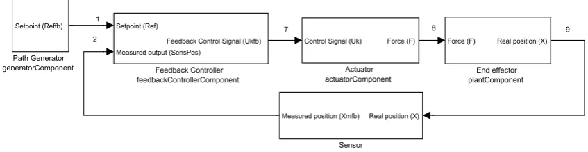
Figure 5.10 shows the connection map. As mentioned in the section 3.5.1, having a connection map can be useful, because of 2 reasons:
1 The connection between components has to be done carefully. The names of each port in every component has to be correct (that is why an assert instruction was used, avoiding mis-spelling is something important).
2 Do not get lost. It can sound funny, but when a component has many input/output ports; having a map can be really useful. Knowing which output port is connected with which input port can avoid future problems. Adding to this, the way it has been programmed makes it easy to connect and disconnect ports.
1 2
7 8 9
Sensor sensorComponent
Real position (X) Measured position (Xmfb)
Path Generator generatorComponent Setpoint (Reffb) Feedback Controller feedbackControllerComponent Setpoint (Ref)
Measured output (SensPos)
Feedback Control Signal (Ukfb)
End effector plantComponent
Force (F) Real position (X)
Actuator actuatorComponent
Control Signal (Uk) Force (F)
FIGURE5.10 - Connection Map of the feedback controller.
The maps can be read in a easy way.
1 Every block represents a component (or agent), and the input and the outputs of the block represent the inputs and the outputs that have been configured in Orocos.
2 The block has two names. One is the generic name, showing which element it represents. The second name shows the component’s Code::Blocks project name.
3 The ports have also two names. The first name represent what identifies the port, and the second one (using parentheses) shows the ports name.
4 Every "wire" between components has a number. This number shows which ports are con-nected and helps to make sure the connection has been done (programming in the correct order makes linking easier).
[image:33.595.73.497.392.502.2]5.8 Simulation results
The simulations have been done using Matlab and Orocos, and comparing the results obtained with each software.
Matlab was created in 1984, and it is known as one of the most powerful and reliable softwares for doing simulations. Orocos was created in December 2000, and is still developing.
First of all, the system behaviour have been analysed. The response of the system with a con-crete setpoint will show if the controller has been tuned in a correct way. Figure 5.11 shows the behaviour of the system simualted with Orocos.
0 0.5 1 1.5 2 2.5 3 3.5
0 0.1 0.2 0.3 0.4 0.5 0.6 0.7 0.8
Time[s]
Position [m]
Response of the simulated system using Orocos
Reference Output
FIGURE5.11 - Setpoint and output comparisson in the simulated system.
As can be seen in figure 5.11 and 5.12, the system behaves in an acceptable way, the maximum error of the system goes from -0.01 to 0.01 meters while the reference is been applied.
Another important aspect of the simulation is the obtained control signal. In figure 5.13 com-parisson is shown between the Matlab simulation and the one done with Orocos.
0 0.5 1 1.5 2 2.5 3 3.5 -0.01
-0.005 0 0.005 0.01
Time[s]
Error [m]
Simulation of the obtained error
FIGURE5.12 - Error of the simulated system.
0 0.5 1 1.5 2 2.5 3 3.5
-0.6 -0.4 -0.2 0 0.2 0.4 0.6
Time[s]
Control signal [V]
Calculated control signal
Matlab Orocos
0 0.5 1 1.5 2 2.5 3 3.5 0
0.5 1 1.5 2 2.5x 10
-3
Time[s]
RMSD of the output of the system [m]
Root mean square deviation between the simulated outputs
6 Learning Feed-Forward controller
6.1 Introduction
A learning controller is a control system that comprises a function approximator of which the input-output mapping is adapted during control, in such way that a desired behaviour of the controlled system is obtained. (22)
As was started in chapter 4, the mathematical model of the system must be "simple enough" so that it can be analyzed with available mathematical techniques, and "‘accurate enough" to describe the important aspects of the relevant dynamical behavior. That is why a moving mass has been taken as a model of simulation. Another factor is that it is known that electromechan-ical motion systems have reproducible disturbances (such as cogging and friction). The main purpose of using a LFFC is to eliminate positional inaccuracy due to reproducible disturbances and model uncertainty.
6.2 LFFC using B-spline Neural Networks
6.2.1 LFFC structures
We consider a controller structure that consists of a feedback and a feed-forward controller. We assume that the state of the process and the state of the reference model are identical and use the approximated inverse dynamics of the process to compute the feed-forward signal. For proper reference signals and when there are no disturbances, if the feed-forward controller equals the inverse of the plant, the tracking error will be zero. The feedback controller is de-signed such that robust stability is guaranteed in the presence of model uncertainty, while the feed-forward controller is used to compensate for known reproducible disturbances. (5)
There are two types of LFFC structures.
• Time Index LFFC: This type of structure is the easiest way of implementing the LFFC. This type of structure can be used for repetitive motions. The main idea of this method is that it learns the control signal that would be needed like a time function (that is why it is used in repetitive motions). Figure 6.1 show the block diagram of the system.
r e u y
Time
Setpoint
Feed-forward Controller
Sensor
Plant Actuator
Feedback Controller
FIGURE6.1 - Time Index block diagram
• State Indexed LFFC: This type of structure is more complex than the Time Index. It can be said that this type of structure is the general form of the LFFC. State Index can be used in repetitive and non repetitive systems. The main idea of this method is that it learns the control signal that would be needed as a function of the states of the systems. So it tries to learn the model uncertainties as function of setpoints states.
Let’s explain it using an example. Suppose that we are working with a system like the one that can be seen in figure 6.2
FIGURE6.2 - A linear process with a non-linearity
The state vector is chosen such that it consists of positions (x2) and their corresponding
velocities (x1) .
· ˙ x1 ˙ x2 ¸ = · A11 I A12 0 ¸ · · x1 x2 ¸ + · B1 0 ¸ ·u
Let’s suppose that the process has both velocity and position dependent non-linearities. This would lead to:
· ˙ x1 ˙ x2 ¸ = · A11 I A12 0 ¸ · · x1 x2 ¸ + ·
h1(x1)+h2(x2)
0 ¸ + · B1 0 ¸ ·u
The desired control signal for a desired position would be:
ud=B1−1·( ¨x2,d−A11·x˙2,d−A12·x2,d−h1( ˙x2)−h2(x2))
As can be seen, the perfect control signal is a function of the plant states.
In theory, the LFFC is able to identy the model uncertainties with the space states; so it would be able to relate the cogging effect with position and friction with velocity for example. So, for a proper learning the setpoints states would be needed, as can be seen in figure 6.3.
r e u y
Setpoint
Feed-forward Controller
Sensor
Plant Actuator
Feedback Controller du/dt
du/dt
FIGURE6.3 - State Index block diagram
In this project Time-index system has been used. The main reason is that from the computa-tional point of view is not more complex to program a state index program, but it takes more time to calculate the algorithm; mainly for two reasons, the first would be that more data is needed (in the time index it has relate control signal to time, in state index it has be relate con-trol signal to the states) and the second would be that more functions should be called, leading to a bigger computational time (this will discussed in this chapter).
6.2.2 LFFC learning
Once the different structures have been briefly explained, we are going to explain how the B-spline NN learns the control signal. The B-B-spline neural network of order N consists of an addition of piece-wise polynomial functions of order n-1.
y(x)= N
X
i=1
ωi·µi(x)
• y: The output of the system that is going to be learned, so the learned signal.
• x: The input of the system. If it is time index, x will be time; if it state index, x will be the states.
• N: Number of B-splines that will be used.
• ω: Weight of the the memberships.
• µ: The membership of the function. The membership is defined by the order of the poly-nomial that will be in charge of approximating the system. Figure 6.4, 6.5, 6.6 show the most common memberships that are used in control enginneering.
The training of the neural network can be done in on-line or off-line mode. In the on-line case, the cost function J is minimized by squared approximation error between the desired output of the BSNydand the actual outputy:
J=1
2·(yd−y)
2
The update of the weights yields:
∆ωi=γ·(yd−y)·µi(x)
FIGURE6.4 - 1storder B-spline
FIGURE6.5 - 2ndorder B-spline
FIGURE6.6 - 3r dorder B-spline
In the off-line training mode, the BSN tries to minimize all the data:
J=1
2· X
j
(yd,j−yj)2
and the weights variation follow the next formula:
∆ωi=γ·
P
j(yd,j−yj)·µi(x)
P
jµni(xj)
The project has been programmed to work in off-line mode as will be explained in section 6.4.
To make sure that the learning concept has been understood, an example will be shown in figure 6.7. It wants to learn the continuosuf f signal using 7 B-splines of 2nd order. uf f is a
time function, and hence in this case x would equal time. Figure 6.4 shows how the continuos
uf f has been approximated by the dotted function.
FIGURE6.7 - Mapping example
6.3 Programming the B-spline: GSL libraries
Programming the neural network can become a complex task, therefore an alternative has been chosen, the GSL libraries (17). The GNU Scientific Library (GSL) is a numerical library for C and C++ programmers. It is free software under the GNU General Public License. The library provides a wide range of mathematical routines such as random number generators, special functions and least-squares fitting. There are over 1000 functions in total with an extensive test suite. Using those functions in an appropiate way will help to obtain a good feed-forward control signal.
6.4 Implementation in Orocos
In this section we are going to explain why the feed-forward is different from the rest of the components and how it has been implemented.
1 Used libraries: When the GSL libraries are used, the project has to look for the Orocos li-braries and the GSL lili-braries. For doing this, first of all the lili-braries have to be installed. The libraries can be found in the GSL’s project main page. After installing them, the project can be ready to know where to look for them. In chapter 3 is explained how to configure Orocos for looking the libraries (steps 15 and 16). Those two lines have to be changed to these ones:
‘pkg-config --errors-to-stdout orocos-ocl-gnulinux orocos-rtt-gnulinux gsl --cflags‘
2 Understanding the code: The comprehension of the example of the GSL page (17) helps to begin understanding the needed functions. The used function in the code will be:
• gsl_vector * gsl_vector_alloc (size_t n)
This function creates a vector of length n.
• gsl_matrix * gsl_matrix_alloc (size_t n1, size_t n2)
This function creates a matrix of size n1 rows by n2 columns.
• gsl_bspline_workspace * gsl_bspline_alloc (const size_t k, const size_t nbreak)
This function allocates a workspace for computing B-splines of order k. The number of breakpoints is given by nbreak.
• gsl_multifit_linear_workspace * gsl_multifit_linear_alloc (size_t n, size_t p)
This function allocates a workspace for fitting a model to n observations using p param-eters.
• int gsl_bspline_knots_uniform (const double a, const double b, gsl_bspline_workspace * w)
This function assumes uniformly spaced breakpoints on [a,b] and constructs the corre-sponding knot vector using the previously specified nbreak parameter.
• double gsl_vector_get (const gsl_vector * v, size_t i)
This function returns the i-th element of a vector v.
• void gsl_vector_set (gsl_vector * v, size_t i, double x)
This function sets the value of x in the i-th element of a vector v.
• int gsl_bspline_eval (const double x, gsl_vector * B, gsl_bspline_workspace * w)
This function evaluates all B-spline basis functions at the position x and stores them in B, so that the ith element of B is Bi(x). B must be of length n = nbreak + k - 2. This function computes the memberships pf all the B-splines.
• void gsl_matrix_set (gsl matrix * m, size t i, size t j, double x)
This function sets the value of x in the (i, j)th element of a matrix m.
• int gsl_multifit_linear (const gsl_matrix * X,
const gsl_vector * y, gsl_vector * c, gsl_matrix * cov, double * chisq, gsl_multifit_linear_workspace * work)
This function computes the best-fit parameters c of the model y = X c for the observa-tions y and the matrix of predictor variables X. So this function can be used to compute weights given the desired output and the memberships.
• void gsl_bspline_free (gsl_bspline_workspace * w)
This function frees the memory associated with the workspace w.
• void gsl_vector_free (gsl vector * v)
This function frees a previously allocated vector v.
• void gsl_matrix_free (gsl matrix * m)
This function frees a previously allocated matrix m.
• void gsl_multifit_linear_free (gsl multifit linear workspace * work)
3 Splitting the code into 3 parts and transferring data among them: The feed-forward con-troller has been divided into 3 parts: data collect, learn and apply; every part has been pro-grammed in a single component. The data collector component is the first and the fastest of the 3 components. Its goal is to collect data and store it in a standard vector. According to Orocos Component Builder’s Manual any type of data can be transferred using ports, so transferring vector is not a problem. The learning part is the main part of the feed-forward controller. The aim of this component is to obtain the weights of the system. For doing this, standard vectors have to be changed to gsl vectors, this can be done using for loops to save the data in the vector and then extract it. The weights are going to be stored in a vector that will be sent to the apply component. The apply is the third component of the feed-forward chain. This component takes the weights, calculates the membership and outputs the ap-propiate feed-forward control signal. This last component is not as fast as the data collect component but it is much faster than the learning component.
4 The use of a non-periodic task: In section 6.6 it will be explained why a non-periodic learning component has to be used. This type of task differs from the rest of the periodic ones, so the way of working will be different. The first thing that has to be done, is adding a Peer from the data collector component to the learn component. For doing this, this line has to be added in the the main program:
feedforwardcontrollerdata->addPeer (feedforwardcontrollerlearn);
After doing that, the task can be configured as a non-periodic one.
NonPeriodicActivity nonperiodicfeedforwardLearnTask(OS::HighestPriority, feedforwardcontrollerlearn->engine());
For running the task:
nonperiodicfeedforwardLearnTask.start();
In this momement, the learning task knows that it is dependent of the data collector compo-nent. The learn component, like any non-periodic activity, would begin to execute once the trigger is fired. For shooting trigger the data collector component has to have these lines of code in its updateHook():
TaskContext* peer = this->getPeer("feedforwardcontrollerlearn"); if (peer != NULL)
peer->engine()->getActivity()->trigger() ;
1 2 9 3 4 5 6 10 11 12 13 14
15 17 16
4 7 8 18 19 20 21 22 23 Sensor sensorComponent
Real position (X)
Measured position (Xm) Measured position (XmData)
Path Generator
generatorComponent
Setpoint (RefData)
Total Time (totalTime)
Period Time (motionTimeDa
ta)
Period Time (motionTime)
Setpoint (Ref)
Total Time (totalTimeD
ata)
Total Time (totalTimeF
F)
Feedback Controller
feedbackControllerComponent
Setpoint (Ref) Measured output (Xm)
Feedback Control Signal
(Ukff)
Feedback Control Signal
(Ukfb)
Feed-Forward Controller Learn
feedforwardControllerLearnComponent
X Parameter (XLearn) Y Parameter (YLearn)
c Parameter (cParam)
Feed-Forward Controller Data Collector
feedforwardControllerDataCollectorComponent
Control Signal (UkLearn) Time (motionTime) Feedback Control Signal
(Ukfb)
x Parameter (X) y Parameter (Y)
Time (motionTimeOut)
Feed-Forward Controller Apply
feedforwardControllerApplyComponent
c Parameter (cParam) Period Time (motionTime) Total Time (motionTime)
Feed-Forward Control Sig
nal (Ukff)
End effector
plantComponent
Force (Force) Time (Time)
Mass (Mass)
Real position (X)
Data
dataComponent
Measured output (Output
)
Setpoint (Setpoint) Total Time (totalTime) Motion Time (motionTime) Feedback control signal
(Ukfb)
Feed-forward control sign
al (Ukff)
Mass (Mass)
Addition Component sumComponent
Feed-Forward Control (Ukf
f)
Feedback Control Signal
(Ukfb)
Control signal (UkLearn)
Feedback Control (UkfbDa
ta)
Feed-Forward Control (Ukf
fData)
Control signal (Uk)
Actuator
actuatorComponent
Control Signal (Uk)
6.5 Learning Signal
The connection map of the feed-forward controller shows that the feedforwardDataCollector-Component has 3 inputs, the periodic time, the total control signal and the feedback control signal. According to some books, the feedforward is tuned with the feedback signal. This can lead to some confussion because it is not clear which signal has to be learnt (there is not going to be a control law in the feed-forward loop, just learning).
Suppose that it is working with a system like 6.9.
R E B U Y
F
P C
FIGURE6.9 - LFFC control diagram
The system can be identified with these equations:
E=R−Y
B=E·C
U=B+F
Y =U·P
Let‘s suppose that the feed-forward control signal can be fully learnt by the total control signal.
F=U
U=B+U→B=0
B=E·C→C6=0→E=0
The control signal is learnt using the equations shown in section 6.2.2. The control signal can be written like:Unew=B+Uol d.
In reality, the signal can not be fully learnt, so this will lead to a small error in the output.
6.6 Learning Component, periodic or non-periodic
When the target of the project was started in section 1.2, an important annotation could be found:"... learning is done asynchronously, in a separate non-realtime Task. ". This annotation makes programming the learning component a bit different to the rest of the component. Does it make any sense having a non-periodic task for the LFFC?
Depending on the amount of data that will be learnt and the number of B-splines, the update-Hook() can take a "long" time to complete. It has to remembered that if an update period of task ishand the computation cost of the updateHook() takes longer thanh, the task will reset before it ends, leading to not calculating the weights and so, not calculating the feed-forward control signal.
The way of working with the non-periodic task will be the next one:
1 The data collector component takes all the data that will be learnt.
2 Shoots a trigger that will wake the learning component.
3 The learning component calculates the weights and loads them in the ports.
4 The apply components loads the weights and calculates, the updated feed-forward control signal.
Some remarks have to be done:
• In a non-periodic task, once the task is started (in the main code, before shuting the trigger), the updateHook() is executed once, and then waits for the trigger.
• The ports keep the values. This leads to an important point, the applying component’s speed is independent of the speed of learning component. The applying component needs the weights for the calculations, but doing the calculations does not take too much time. The applying component is waiting two periodic cycles to begin running, in this way we could be sure that some weights will be learnt (after the first periodic cycle, learn-ing component is launched and its execution will take less than one periodic cycle). After the first updateHook() in the applying component, the values of the weights keep in the ports until the learn component changes them (one data collecting cycle plus the calcu-lations of the learning component). Thanks to this, the data collector component and the apply component can almost go to the same speed as the feedback loop.
6.7 Results
The program allows the user change several parameters of the simulation.
• The amount of data that has to be learnt: Refers to the amount of data that will be saved in vectors. The vectors that have been used have a fixed size. This parameters is related to the refresh rates of the data collector component and the apply component. Having a small refresh rate can force to an updateHook() not to finish its execution, leading to a bad behaviour of the controller.
• The order of the B-spline. In subsection 6.2.2, it was explained that the membership parameter can go from an order 1 polynomial to higher order polynomials. In the code, the order of the system can be changed just changing one value.
• The number of B-splines that are going to be used. This parameter can be checked in learning and applying components. As it has been said before, the learning component is non-periodic, so the calculation time that will need it is not important, but the apply component also needs this parameter. Having a big number of B-splines can make cal-culating the feed-forward control signal take too long, if the refresh rate is faster than the time needed to calculate the system, the feed-forward is not going to be applied (the previous period result will remain in the port).
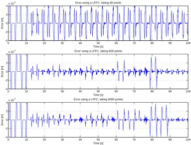
Two conclusions can be achieved with this parameter variation. The first would be that a low number of data makes the data not accurate enough to learn. The second would be that a too high number of data, implies a longer time of learning. If a big change is done in the system, it takes 2 periods to reduce the error using 6000 points, but if 600 points are used the error reduces after 1 period. The 600 points configuration has be chosen.
0 10 20 30 40 50 60 70 80 90 100
-4 -2 0 2 4x 10
-3 Error using a LFFC, taking 60 points
Time [s]
Error [m]
0 10 20 30 40 50 60 70 80 90 100
-4 -2 0 2 4x 10
-3 Error using a LFFC, taking 600 points
Time [s]
Error [m]
0 10 20 30 40 50 60 70 80 90 100
-4 -2 0 2 4x 10
-3 Error using a LFFC, taking 6000 points
Time [s]
Error [m]
FIGURE6.10 - Error of the system with different amount of data to fit
The second parameter that is going to be studied is going to be order of the B-spline. In 6.2.2 could be checked the different order of the membership parameter. In one hand a higher mem-bership can mean a more smooth fitting, but in the other hand, a higher computational cost. Figure 6.11 shows obtained results. According to the results, there is not a big difference be-tween a second and a third order B-spline. As the results are almost the same, and the third order BSN takes more time of calculation, the second order B-spline has been chosen.
[image:48.595.122.506.154.445.2]0 10 20 30 40 50 60 70 80 90 100 -4
-2 0 2 4x 10
-3 Error using a LFFC, B-spline of order 1
Time [s]
Error [m]
0 10 20 30 40 50 60 70 80 90 100
-4 -2 0 2 4x 10
-3 Error using a LFFC, B-spline of order 2
Time [s]
Error [m]
0 10 20 30 40 50 60 70 80 90 100
-4 -2 0 2 4x 10
-3 Error using a LFFC, B-spline of order 3
Time [s]
Error [m]
FIGURE6.11 - Error of the system with different order B-splines
0 10 20 30 40 50 60 70 80 90 100
-4 -2 0 2 4x 10
-3 Error using a LFFC, 32 B-splines
Time [s]
Error [m]
0 10 20 30 40 50 60 70 80 90 100
-4 -2 0 2 4x 10
-3 Error using a LFFC, 50 B-splines
Time [s]
Error [m]
0 10 20 30 40 50 60 70 80 90 100
-4 -2 0 2 4x 10
-3 Error using a LFFC, 64 B-splines
Time [s]
Error [m]
After doing several simulations and analyzing the data, the used configuration has been the next one:
• Speed of the feedback loop (setpoint, feedback controller, actuator, plant, sensor, addi-tion and data component): 10 kHz.
• Speed of the feed-forward controler (data collect and apply): 100 Hz.
• Speed of the reporter component: 1 kHz.
• The setpoint is periodic every 6 seconds.
• The learning component starts working after the first cycle.
• The applying component starts working after the second cycle.
• Amount of data that will be learnt: 600 points.
• Number of B-splines that will be used: 50.
• Mass of the model: 0s≤t<24s→m=10kg
24s≤t<42s→m=11kg
42s≤t<60s→m=10kg
60s≤t<78s→m=12kg
78s≤t<100s→m=9kg
For a better analysis of the data the next two tables are given. The convergence of the error using the LFFC makes the error reduce 13 times compared to the feedback controller. Another thing that can be checked in the tables is that the feedback and the feed-forward control signals react to the mass variation. With the used algorithm, the feed-forward controller takes one period to learn the data. After doing learning, it reduces the error and the control signal stabilizes.
Time [s] Mass [kg] Feedback Signal [V] Feed-forward Signal [V]
0≤t<12 10 [-0.5115 , 0.5115] [0,0]
18≤t<24 10 [-0.0970 , 0.0680] [-0.4702,0.4702]
24≤t<30 11 [-0.0680 , 0.0920] [-0.5302,0.5302]
36≤t<42 11 [-0.0950 , 0.0580] [-0.524,0.524]
42≤t<48 10 [-0.1400 , 0.0830] [-0.522,0.522]
54≤t<60 10 [-0.1052 , 0.0540] [-0.4724,0.4724]
60≤t<66 12 [-0.1054 , 0.1384] [-0.5855,0.5855]
72≤t<78 12 [-0.1260 , 0.0875] [-0.5855,0.5855]
78≤t<84 9 [-0.2350 , 0.0181] [-0.4228,0.4228]
90≤t<96 9 [-0.0850 , 0.039