An Approach to Parallelization of SIFT Algorithm on GPUs for Real Time Applications

(1)

http://www.scirp.org/journal/jcc ISSN Online: 2327-5227

ISSN Print: 2327-5219

An Approach to Parallelization of SIFT

Algorithm on GPUs for Real-Time Applications

Raghu Raj Prasanna Kumar, Suresh Muknahallipatna, John McInroy

Department of Electrical Engineering, University of Wyoming, Laramie, USA

Abstract

Scale Invariant Feature Transform (SIFT) algorithm is a widely used comput-er vision algorithm that detects and extracts local feature descriptors from images. SIFT is computationally intensive, making it infeasible for single threaded implementation to extract local feature descriptors for high-resolution images in real time. In this paper, an approach to parallelization of the SIFT algorithm is demonstrated using NVIDIA’s Graphics Processing Unit (GPU). The parallelization design for SIFT on GPUs is divided into two stages, a) Al-gorithm design-generic design strategies which focuses on data and b) Im-plementation design-architecture specific design strategies which focuses on optimally using GPU resources for maximum occupancy. Increasing memory latency hiding, eliminating branches and data blocking achieve a significant decrease in average computational time. Furthermore, it is observed via Pa-raver tools that our approach to parallelization while optimizing for maxi-mum occupancy allows GPU to execute memory bound SIFT algorithm at optimal levels.

Keywords

Scale Invariant Feature Transform (SIFT), Parallel Computing, GPU, GPU Occupancy, Portable Parallel Programming, CUDA

1. Introduction

Image matching is a fundamental aspect needed to solve computer or machine vision problems, including object or scene recognition, 3D structure modeling, stereo image correspondence, motion tracking, etc. Objects in images have fea-tures that can be extracted and used for comparing across images. A large num-ber of such features for various objects can be extracted from images with

effi-How to cite this paper: Kumar, R.R.P., Muk- nahallipatna, S. and McInroy, J. (2016) An Approach to Parallelization of SIFT Algo-rithm on GPUs for Real-Time Applications. Journal of Computer and Communications, 4, 18-50.

http://dx.doi.org/10.4236/jcc.2016.417002

Received: October 25, 2016 Accepted: December 26, 2016 Published: December 29, 2016

http://creativecommons.org/licenses/by/4.0/

(2)

cient algorithms. An example of such an algorithm is Scale Invariant Feature Transform (SIFT) [1], which detects and extracts local feature descriptors from images. The features extracted using the SIFT algorithm are invariant to rotation, scaling and illumination and hence applicable to scene modeling, recognition and tracking [2]. A simple sequential implementation of SIFT on lower resolu-tion images is shown to utilize huge memory with high computaresolu-tion times [3], making the use of SIFT in real-time applications infeasible.

High-resolution image processing is used in various application domains like remote sensing, traffic monitoring, unmanned air vehicles, mars expeditions, etc. SIFT has been shown to provide good tracking capability in all the above do-mains [4][5][6][7]. However, the large computational burden prevents the use of SIFT in real-time applications in the above domains. Feng et al., in their mul-ti-core parallelization work [8] have demonstrated the potential of parallelizing the SIFT algorithm. A number of researchers [3][9][10]-[15][35][36][37][38] [39] have attempted to parallelize the SIFT algorithm to make it applicable for real-time. In particular, the research effort by Yao et al., has demonstrated a pa-rallelized SIFT algorithm [13] with the capability to process an image of resolu-tion 640 × 480 pixels in 31 ms. The 31 ms processing time would be sufficient to process video of frame rate 24 frames per second with a resolution of 640 × 480. However, the current application domains require processing of images with resolutions ranging from 1280 × 720 (720 p) to 8192 × 4608 (8 k) known as high- resolution images in real-time. Recent researches [16] [17][18] [19][20] have attempted to parallelize SIFT for high-resolution images. However, all of these attempts either have high execution time or fail to provide reproducible imple-mentation, making current approaches of parallelizing the SIFT algorithm in-compatible for real-time applications.

In this paper, we discuss a two phase: a) algorithm design and b) implementa-tion design, parallelizaimplementa-tion strategies to obtain a better and efficient paralleliza-tion of SIFT, which lowers the compute time enabling real-time processing of high-resolution images. While, the algorithm design phase strategies demon-strate parallelization of the SIFT algorithm, the implementation design phase strategies define the values of machine parameters, such as blocks and threads, to implement the parallelized SIFT algorithm on to the underlying GPU archi-tecture. The two-phase parallelization approach facilitates porting of parallelized SIFT algorithm to different GPU architectures. The research work presented in this paper is based on the preliminary research presented by authors in [21]. In preliminary research, the parallelization of only the first stage of the SIFT algo-rithm was presented. This paper presents the complete parallel implementation of SIFT suitable for real-time applications.

(3)

intro-duction to the GPU architecture and its constraints are presented. In Section 5, we provide the two phase parallelization strategies and demonstrate the paralleli-zation of SIFT algorithm. Section 6 provides the performance of the parallelized SIFT algorithm. We discuss the future work and conclude the paper in Section 7.

2. Description of SIFT

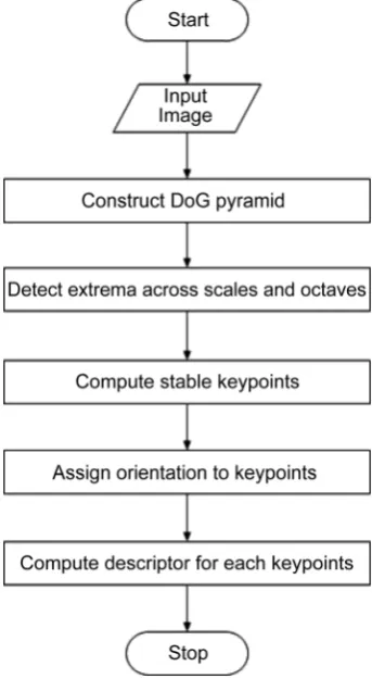
[image:3.595.287.459.374.687.2]

SIFT algorithm discussed in the research work by Lowe has four stages to obtain the features of an image [1]. The four stages of the SIFT algorithm are shown in

Figure 1. A discussion of the four stages is provided below:

1) Scale-space Extrema Detection (SSED): The SSED stage consists of two sub-stages namely the formation of the Difference of Gaussian (DoG) pyramid and extrema keypoint detection.

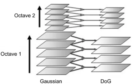
a) Difference of Gaussian Pyramid: The first stage of computation is to build a pyramid of images having different blurring levels and varying resolutions. First, the initial image is repeatedly convolved with different Gaussian functions cha-racterized by their varying standard deviations known as scaling, to produce a set of images having same resolution but varying in their blurring levels as shown in Figure 2. In Figure 2, this set of images is marked as Octave 1 representing the same resolution but different blurring levels. The top image of octave 1 has

(4)

[image:4.595.260.488.65.210.2]

Figure 2. DoG pyramid structure.

the maximum blurring. Next, the resolution of the top image in Octave 1 is re-duced by half to form the bottom image in Octave 2. Again, this bottom image in Octave 2 is repeatedly convolved with different scaled Gaussian functions to produce the set of images for Octave 2. This convolution and resolution reduc-tion is repeated to build the different layers of the pyramid. Next, the DoGs of an octave are constructed by taking the difference between any two consecutive images of the same. The left side in Figure 2 depicts the different octaves and scaled images in each octave, and the right side depicts the corresponding DoG images. Interest points for SIFT are obtained using the DoG images.

b) Extrema detection: The pixels of a DoG image are the difference in intensi-ty values of consecutive blurred images. Keypoints are pixels identified as local maxima or minima of the DoG images across octaves. This is obtained by com-paring a pixel in the DoG image to its neighboring pixels at the current and ad-jacent scales [1]. If the pixel is greater than or lesser than all its neighbors, it is considered as the local maxima or minima respectively for the given octave level. If the local minima or maxima for the first octave, continues to be a local mini-ma or mini-maximini-ma for all octaves, then it is selected as a candidate keypoint.

2) Keypoint localization: The selected candidate keypoints (CKs) are filtered to eliminate unstable CKs. CKs having low contrast or being a part of an edge in an image are considered as unstable keypoints [1]. A 3D quadratic function fit-ting is performed on the selected CKs to evaluate its contrast with respect to neighboring points [22]. By setting a threshold for evaluation, low contrast CKs are eliminated [1]. A second-order derivative of the Hessian matrix [1] is used to eliminate the CKs that form part of an edge.

(5)

3. Steps in SIFT

A step-by-step mathematical discussion of SIFT, as seen in [1], is provided be-low. It should be noted that we are reiterating the description of SIFT from [1], without adding any new terminologies or techniques.

a) Gaussian convolution: Consider a Gaussian matrix s 3 3

G ∈R× , given by:

(

2 2

)

2 2 2 1 e 2π s i j s ij s G σ σ − +   =  

  (1)

where, 1

2s s

σ =σ is the standard deviation at every scale,

0.8

σ

= is the predetermined standard deviation for the SIFT algorithm, and s is the scaling level,

{

}

, 1, 0,1

i j= − are the indices of Gs, with

( )

0, 0 being the element under- going convolution operation.

( )

0, 0 is the index of the middle element of Gs matrix.

Gs_{is convolved with the grayscale image} _o _mo _no

I ∈R × , where o is the octave level, m no, o is the resolution of the image for the octave level o. The

convolu-tion is performed by sliding Gs_{as a window over} o

I . The convolved image

o o

so m n

L ∈R × , is obtained as follows:

*

so s o

xy ij xy

L =G I (2)

where, x y, in o xy

I and Lso_xy is the co-ordinate of a pixel in the image.

Since the image values are discrete numbers, the convolution is performed as shown below:

( )( )

3 3

1 1

so s o

xy ij x i y j

i j

L G I ₋ ₋

= =

=

∑∑

₍₃₎

b) DoG computation: The difference between so

L of two consecutive scale levels, s1 and s2, provides a corresponding DoG _Ds21o, as shown below:

21 2 1

s o s o s o

xy xy xy

D =L −L (4)

This operation can be merged as shown in Equation (5) eliminating one mul-tiplication per pixel in _Io.

(

)

21 2 1

*

s o s s o

xy ij ij xy

D = G −G I (5)

c) Scaling: Once _Ds21o for all scales of an octave are computed, the last _Lso

is scaled down by 2 to obtain o 1

I + .

d) Pyramid construction: The steps (a), (b) and (c) are executed for _Io+1 to

obtain o 2

I + and so on. This whole process is repeated till a preset octave level is obtained. For the purpose of this paper o = 4 and s = 4, is used based on the dis-cussions in [1].

(6)

images. For every DoG image in an octave, the maxima and minima are detected by comparing a pixel (indicated by a triangle) to its twenty six neighbors com-prising of 3 × 3 × 3 region at the current and adjacent scales (indicated by circles) as shown in Figure 3.

f) Low contrast keypoint elimination: The extrema detection provides a set of CKs that include points having low contrast or are poorly localized along an edge, and hence are considered unstable [1]. To eliminate low contrast CKs, an evaluation of CKs’ contrast with respect to its neighboring points needs to be determined. This is done by fitting a 3D quadratic function to the CK as de-scribed in [1][22]. The 3D quadratic function is given by:

( )

T T 2

2

1 2

D D

D Χ = +D _∂ _ Χ + Χ ∂ Χ

∂Χ ∂Χ

  (6)

where,

[

]

T

x y σ

Χ = _,

21

s o xy

D∈D ,

D D D D

x y σ

 

∂ ∂ ∂ ∂

=  

∂Χ _∂ ∂ ∂ _,

2 2 2

2

2 2 2 2

2 2

2 2 2

2

D D D

x y x

x

D D D D

x y y y

D D D

x y

σ

σ σ σ

∂ ∂ ∂   _∂ _{∂ ∂} _{∂ ∂}      ∂ _{= }∂ ∂ ∂  ∂ ∂ ∂ ∂

∂Χ  ∂ 

_∂ _∂ _∂ 

 

∂ ∂ ∂ ∂ ∂ 

 

Since the image values are discrete numbers, the derivatives have to be com-puted numerically. Equations (7)-(9) provide the finite difference method to cal- culate the partial derivatives , 22

D D

x x

∂ ∂

∂ ∂ and

2

D x y ∂

[image:6.595.261.490.542.690.2]

x − +

∂

= − −

∂ (7)

( ) ( )

2

1 1

2 2

so so so

xy

x y x y

D

L L L

x + −

∂

= + −

∂ (8)

( )( ) ( ) ( ) ( ) ( ) ( )( )

2

1 1 1 1 2 1 1 1 1

2

so so so so so so so

xy

x y x y x y x y x y x y

L L L L L L L

D

x y

+ + − + − + + − − − − + − −

∂ ₌

∂ ∂ (9)

The contrast

(

_D

( )

_Χˆ

)

_{of the CK w.r.t. neighboring pixels is evaluated by}

calculating the function value at the extremum position

( )

_Χˆ _{as shown in}

Equ-ations (10)-(11):

( )

T

1

ˆ ˆ

2 D

D Χ = +D _∂ _ Χ

∂Χ

  (10)

1 2

2

ˆ D D

−

∂  ∂

Χ = −_∂Χ _{ ∂Χ}

  (11)

The CKs are considered low contrast if they satisfy the inequality shown in Equation (12) and are discarded.

( )

ˆ _0.03

D Χ < (12)

g) Edge keypoint elimination: The DoG has a strong edge response, i.e., points on an edge is detected as an extrema. This is due to the principal curvature val-ues for DoG tend to be higher along an edge. However, the principal curvature value for DoG along the perpendicular direction of an edge is low in magnitude. This property is used to eliminate the CKs that are a part of the edge. The eigen values of the Hessian matrix

( )

H computed on D, as shown in Equation (13), are proportional to the principal curvature values.

2 2 2 2 2 2 D D x y x H D D

x y y

∂ ∂  _∂ _{∂ ∂}    =_ _ ∂ ∂   ∂ ∂ ∂     (13)

2 2

1 Det

Tr H r

H r

+

< ₍₁₆₎

(8)

h) Orientation assignment: The keypoints can be described relative to local orientation of its neighboring pixels rendering them invariant to image rotation. The orientation is assigned by calculating two parameters a) gradient magnitude

( )

m and b) gradient orientation

( )

θ . For a given keypoint

(

x y,

)

, orientation is assigned as follows:

( ) ( )

(

)

(

( ) ( )

)

2 2

1 1 1 1

so so so so

xy x y x y x y x y

m = L ₊ −L ₋ + L ₊ −L ₋ (17)

( ) ( ) ( ) ( ) 1 1 1 1 1 tan so so

x y x y

xy so so

x y x y

L L

θ

− + −

+ −

 − 

 

=

 − 

  (18)

A descriptor is generated using this orientation by constructing a histogram of orientations of sample points around the keypoints. Each sample point added to the histogram is weighted by its gradient magnitude and Gaussian-weighted circular window proportional to the σ of the keypoint scale. This generates a vector of values termed as keypoint descriptor. The keypoint descriptor is the scale, orientation, and location invariant data set obtained as the output of SIFT algorithm.

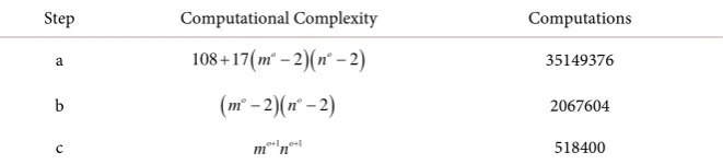
From an implementation perspective, steps (a), (b), (e), (f), (g) and (h) involve arithmetic computations, while steps (c) and (e) involve assignment and com-parison operations. Since, assignment involves a memory write, requiring more cycles than a single floating point operation, every write in step (c) is considered as one computation for the purpose of this paper. Steps (e) - (h) are dependent on the number of CKs and keypoints computed in an image. On a per keypoint basis, the number of computations involved for steps (e) - (h) are in the order of hundreds. Steps (a) - (c) have large number of computations, independent of the CKs and keypoints generated. Since, the number of CKs and keypoints com-puted are fewer in number, steps (a) - (c) form a significant overhead compared to steps (e) - (h). The computations involved in steps (a) - (c) are shown in Table 1 for a standard high definition image with resolution of 1

1080

m = , n1=1920

at octave level 1. From the table, the computational complexity for steps (a) - (c)

can be formulated as 4

(

)(

)

1 1

1

432 18 o 2 o 2 o o

o

m n m +n+

=

+

∑

− − + _{. If the steps (a) - (d)}

[image:8.595.208.539.628.703.2]

generate k keypoints, then computations for (e) - (h) are Ο

(

100k

)

. Hence, the computations shown in Table 1 indicate that our parallelization should focus more on steps (a) - (c).

Table 1. Step-wise computations for SSED for octave level 1.

Step Computational Complexity Computations

4. Compute Unified Device Architecture

General-Purpose Computing on GPU (GPGPU) is a new parallelization domain to accelerate scientific and engineering computations in vision algorithms [23]. NVIDIA’s CUDA is the earliest and most widely adopted programming model for GPGPU [24]. Since the beginning of parallelization on GPGPU, NVIDIA has introduced several GPU architectures to improve the performance of parallelized programs. An overview of the three common features of GPU architecture namely thread, memory and execution hierarchies [25], are provided below.

GPU thread hierarchy is characterized by three parts namely the grid, block

( )

B and thread

( )

T . Each grid contains 1D, 2D or 3D arrangement of blocks and each block contains 1D, 2D or 3D arrangement of threads. The number of threads per block cannot vary across blocks. Hence the total number of threads spawned is the product of total blocks and threads per block.

GPU memory hierarchy has three classifications namely the register

( )

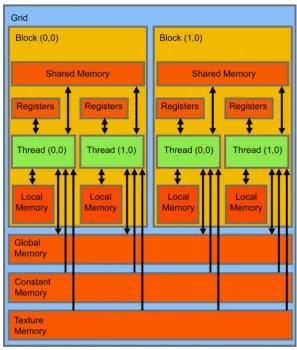
ρ _,

[image:9.595.223.521.326.677.2]

shared

( )

ψ and global memories. The memory hierarchy and its accessibility with respect to threads and blocks are shown in Figure 4.

(10)

Each thread within a block has access to private register memory, and all the threads within a single block have access to the shared memory, through which they share data. The threads distributed across multiple blocks have access to global memory, but sharing or visibility of modified data across blocks is not guar-anteed. The memory access latency increases non-linearly from register memory to global memory thereby an excessive use of global memory leads to computa-tional penalties. However, the amount of memory also decreases non-linearly from global to register memory. Furthermore, it is possible to achieve efficient memory bandwidth usage if the data on global memory is arranged for coalesced access.

In addition to the above three types of memories, there are two additional read-only memory types accessible by all threads known as constant and texture memories. The constant and texture are GPU memories that are cached and op-timized for read access. While the constant memory is opop-timized to access data elements of limited size, the texture memory is optimized for scattered access of large data.

The instruction execution hierarchy of GPUs consists of a set of streaming multiprocessors (SMs) with each SM containing multiple execution cores

( )

C . Based on the number of cores, each SM can concurrently execute a limited num-ber of threads known as a warp

( )

w . The warp organization represents the Sin-gle Instruction Multiple Threads (SIMT) architecture. Hence, combining the number of warps per SM and the number of SMs per GPU, increases compute parallelization and effective utilization of memory bandwidth. However, due to SIMT architecture, SM executes instructions with a granularity of a warp, i.e.; all threads within a warp execute the same instruction

( )

ϕ _{. However, conditional}

flows due to the nature of the algorithm may introduce conditional branches within a single warp contributing to the increase in computation time.

The scalability of CUDA lies in the execution model. While blocks and threads form the partitioning of workload, the execution model provides a feature to map the threads to SMs. Based on the number of blocks and threads per block, a scheduler allocates one or more blocks to each SM. The number of blocks that can execute concurrently on a SM is based on the number of warps that can con-currently execute on the SM which, in turn, is based on the amount of maximum warps supported by the SM, and the amount of shared and register memory re-quired by a block. As the memory requirement per block increases, the number of warps that can concurrently execute on a SM decreases. An SM is said to be at maximum efficiency if the number of warps concurrently executing is equal to maximum warps supported by the SM.

(11)

Constraints, for the purpose of this paper, are represented symbolically as a func-tion shown below:

(

, ,

)

η α β γ =δ₍₁₉₎

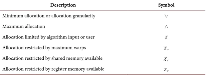
where α represents the variable to which the constraint applies, β represents the scope of the α variable, γ represents the type of restriction imposed on α and δ is the output that provides the numerical value of the restriction. γ can take the fol-lowing values listed in the Table 2 below.

Table 3 summarizes all the thread and execution hierarchy based constraint

[image:11.595.209.540.248.368.2]

functions:

Table 2. List of restrictions imposed on constraint functions.

Description Symbol

Minimum allocation or allocation granularity ∨

Maximum allocation ∧

Allocation limited by algorithm input or user χ Allocation restricted by maximum warps χw

Allocation restricted by shared memory available χψ

[image:11.595.201.537.397.722.2]

Allocation restricted by register memory available χρ

Table 3. List of execution hierarchy based constraint functions.

Description Function

Maximum SMs per GPU η(SM GPU, ,∧)

Allocated blocks per GPU η(B GPU, ,χ)

Maximum active blocks per SM η(B SM, ,∧)

Maximum warps per SM η(w SM, ,∧)

Maximum active threads per SM η(T SM, ,∧)

Allocated blocks per SM η(B SM, ,χ)

Allocated warps per SM η(w SM, ,χ)

Allocated warps per SM based on χw η(w SM, ,χw)

Allocated warps per SM based on χσ η

(

w SM, ,χψ

)

Allocated warps per SM based on χρ η

(

w SM, ,χρ

)

Maximum threads per block η(T B, ,∧)

Allocated warps per block η(w B, ,χ)

Allocated threads per block η(T B, ,χ)

Maximum threads per warp η(T w, ,∧)

(12)

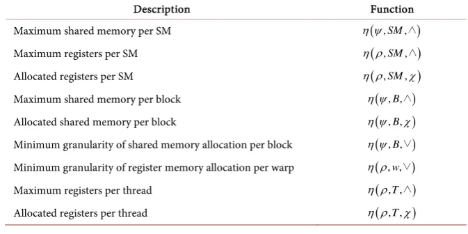
Similar to SM, B, T and w, the memory is also subjected to constraints. Table 4

summarizes all the memory hierarchy based constraint functions:

5. Parallelization

There have been a number of GPU parallelization strategies that have been pro-posed over the last few years. A few relevant to SIFT are presented in [26]-[34]. While [26] [27] focus on parallelization strategies for stencil codes similar to SIFT, [28]-[34] focus on implementation specific strategies for parallelization. None of the articles provide algorithm design strategies, as we propose in this paper, to utilize the benefits of GPU architecture for parallelization.

The parallelization strategies, proposed in this paper, are divided into two phases for separating SIFT and GPU related parallelization strategies. The algo-rithm design phase strategies focus on parallelizing SIFT based on data size, data usage, and data organization. The implementation design phase strategies focus on how the parallelized SIFT design can achieve maximum execution efficiency on a GPU. The remainder of this section focuses on the description of the two phases and their application on SIFT.

The algorithm design phase strategies involve parallelization techniques based on three guidelines.

[image:12.595.203.540.541.709.2]

a) Reduce: As seen in [35], the bottleneck of algorithm execution is always found to be the memory accesses-read and write operations. The memory opera-tions require higher time reducing the performance of the algorithm. Hence, the higher the number of memory operations, the lower the performance of the al-gorithm. However, not all algorithms’ performance is bound by memory. This is because algorithms may have a lot more computations than memory operations. In order to differentiate memory bound algorithms, a ratio, termed as computa-tional intensity (CI), is defined as the number of floating point computations performed for each memory operation. This provides a measure to understand the impact of memory operations on algorithms. It is given by

Table 4. List of memory hierarchy based constraint functions.

Description Function

Maximum shared memory per SM η ψ( ,SM,∧)

Maximum registers per SM η ρ( ,SM,∧)

Allocated registers per SM η ρ( ,SM,χ)

Maximum shared memory per block η ψ( , ,B∧)

Allocated shared memory per block η ψ( , ,Bχ)

Minimum granularity of shared memory allocation per block η ψ( , ,B∨)

Minimum granularity of register memory allocation per warp η ρ( , ,w∨)

Maximum registers per thread η ρ( , ,T∧)

(13)

Number of floating point computations CI

Number of memory operations

= ₍₂₀₎

The CI determines if an algorithm is memory or compute bound. If the ratio is less than 1, then it is said to be memory bound. For CI0, the algorithm

tends to become compute bound.

The reduce guideline states that for a memory bound algorithm, the number of memory operations should be reduced to increase CI. In other words, for every floating point operation, the number of memory operations should be mi-nimized. This can be achieved either by a) computing values rather than loading or b) reducing memory latency by grouping algorithm’s data. While (a) replaces the memory operations with floating point computations, (b) groups floating point operations such that they operate on common memory elements.

The SIFT algorithm, inferring from steps (a) - (c) and (e) - (g) in section III, is a memory bound algorithm. For example, step (e) alone in section III requires 27 loads for detecting extrema.

b) Reuse: Commonly known as cache blocking, this guideline states that reu-sability of memory elements should be maximized, i.e., a memory element loaded should not have to be reloaded during any part of the execution. This can be achieved by grouping algorithmic operations such that all computations asso-ciated with a memory element are performed together.

The SIFT algorithm has high data reusability. For example, step (c) seen in section III shows that 25% of the image data is re-used for every octave.

c) Re-arrange: Scattered memory operations result in poor utilization of memory bandwidth. This guideline recommends rearranging instructions and data to avoid branching of execution and increase memory bandwidth usage re-spectively.

SIFT algorithm is observed to have both branching and scattered data access. For example, while step (d) in section III requires twenty six comparisons, lead-ing to branchlead-ing, step (d) scatters data elements for an increase in octave level.

These guidelines are not rigid rules but rather provide a methodology to par-allelize programs. The SSED parallelization, steps (a) - (e) in section III has been parallelized in our previous work-in-progress publication [21]. However, the adoption of guidelines has improved upon the parallelization strategies as shown below:

(14)

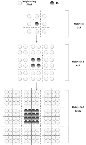
high resolution images. Adhering to our guidelines, we propose top-down ap-proach for parallelization of SSED; we group data based on the top DoG image in the highest octave. To determine if s21o

xy

D at the highest octave and scale is an extrema, it has to be compared to eight neighboring pixels of the same scale, and eighteen neighboring pixels of adjacent scales within the same octave level. Adopting reduce guideline, all scales within an octave can be computed simul- taneously. Therefore SSED would require loading nine elements-eight neigh-boring pixels and the s21o

xy

D itself. Adopting the reuse guideline-instead of re- loading the elements for each octave, reusing these elements across octave is recommended. However, data dependency between neighboring pixels from a lower octave level is observed, i.e., in order to retain the eight neighboring pixels in the current octave, thirty six data neighboring pixels are required from the previous octave. Similarly, dropping down to lower octave levels, a fourfold in-crease in data elements is observed as shown in Figure 5. With o = 4, this would be 24 × 24. Adopting the re-arrange and reduce guideline, if threads can be grouped to share data, then the neighboring elements are grouped together to have common elements.

b) Next, finding the minima/maxima requires twenty six comparisons. The twenty six comparisons at every octave level results in divergence between the threads belonging to the same warp. This will prevent concurrent execution of threads in a warp [36] and hence increases the computational time. Hence, adopting the re-arrange guideline, the twenty six comparisons are replaced with a single comparison reducing the multiple divergences to a single divergence. Consider a pixel a∈N which needs to be compared with twenty six other pix-els represented as ax, where x=1, 2,, 26 and ax∈N. To check whether

a is maxima or minima, the two factors given in Equations (7), (8) are com-puted: 26 x x a a

α

    =     

∏

 (21) 26 x x a a

β

    =      

∏

(22)

Next, If α > 0 and β = 0 then a is the local maxima and if β > 0 and α = 0 then a is the local minima.

(15)

[image:15.595.219.522.72.581.2]

Figure 5. Top down view of number of data elements needed to compute the extrema for three octave levels.

(16)

together into a new matrix structure, eliminating all irrelevant data. The organi-zation of the new matrix structure can vary based on the underlying architecture support. For example, if the underlying architecture supports interleaved mem-ory accesses between thread, similar to GPU SIMT architecture, the elements can be arranged in an interleaved fashion, i.e., first data element accessed by every thread are grouped together followed by second element used by all threads and so on. If the underlying architecture supports consecutive memory accesses per thread, similar to CPU SIMD architecture, then all elements used by single thread are grouped together. A map between the new data layout and the origi-nal image is retained to re-map the descriptors back to origiorigi-nal image.

Since there are no dependencies observed in steps (e) - (h) described in sec-tion III, the computasec-tion at hand is embarrassingly parallel with respect to each keypoint. Moreover, each keypoint requires no more than 8 neighboring pixels for all computations through steps (e) - (h) per scale per octave leading to a high CI.

As mentioned earlier, this algorithm design phase facilitates for parallelization of SIFT algorithm across architectures. The second phase of parallelization in-volves implementation design parallelization strategies. There are several differ-ent approaches to designing parallelization strategies for GPU. Two popular ap-proaches, as seen in [26]-[34], are a) Maximizing occupancy and b) Maximizing memory bandwidth. Our approach for implementation design phase is max-imizing occupancy as opposed to maxmax-imizing memory bandwidth. This is be-cause our approach to eliminating memory bottlenecks at algorithm design phase complements a maximizing occupancy in implementation phase.

)

(

)

η

χ

=

η

χ η

χ

η

χ

(24)

(

w SM, , _w

)

η χ depends on the limitation of warps per SM and the maximum

active blocks per SM as observed in NVIDIA’s documentation. η

(

w SM, ,χw

)

is decided as the minimum of two values: a) The number of warps needed to ex-ecute the allocated blocks and b) Maximum warps on a SM. It is computed using the Equation (25) below:

(

, ,

)

min

(

₍

, ,

₎

)

(

, ,

) (

, , ,

)

, ,

w

w SM

w SM w B w SM

w B

η

η χ η χ η

η χ    = _  _       ∧

∧ (25)

where,

(

, ,

)

(

₍

, ,

)

₎

, , T B w B T w η χ η χ η   =    

₎

, ,

ceil , , , , ,

SM w SM B B ψ

η ψ

η

χ

η ψ

χ η ψ

 

=  

 

 

∧

∧ (27)

Due to hardware constraints, shared memory has allocation granularity, i.e., the allocation of shared memory is always an integral multiple of η ψ

(

, ,B∨

)

. The ceil function rounds the first argument to the immediate next multiple of the second argument. In Equation (27), the allocation of shared memory per block is rounded to allocation granularity using ceil function.

(18)

calcu-lated as shown below:

(

)

(

₍

, ,

₎

)

(

)

, , , ,

, , SM

w SM w B

w B ρ

η ρ χ

η χ η χ

η χ

 

=  

 

  (28)

where,

(

, ,

)

₍

_{) (}

(

, ,

)

_{) (}

₎

ceil , , , , , , ,

SM SM

T T w w

η ρ

χ

η ρ

χ η

η ρ

 

=  

 

 

∧

values that can be used.

b) Select blocks to maximize occupancy: The blocks on a GPU tend to in-crease the number of floating point operations performed rather than hide the memory latency. Hence choosing higher blocks improves compute bound algo-rithms performance. The feasible blocks is calculated using:

(

, GPU,

)

₍

_{) (}

₎

min , , , , ,

N B

T B N B

η χ

η χ η χ

= ₍₃₀₎

where, N represents the total number of data elements. Since SIFT is a memory bound algorithm, we only focus on the scenario when CI < 1. If CI < 1 then se-lecting η

(

T B, ,χ

)

with the highest value, and its corresponding η

(

B, GPU,χ

)

would provide better performance as increased threads per block promote memory latency hiding.

The above guidelines are based on the assumption that the total number of data points N≤η

(

B, GPU,χ η

) (

T B, ,χ

)

. If otherwise, it is recommended to increase η ϕ

(

, ,T χ

)

till Equation (31) provides blocks and threads within GPU constraints.

(

, GPU,

)

₍

_{) (}

₎

, , , ,

N B

T B T

η χ

η χ η ϕ χ

= ₍₃₁₎

The two guidelines in the implementation design phase provide the exact thread and block numbers that maximizes performance on GPU. Since the cal-culations depend on the GPU used, image resolution and the number of key-points generated, its calculation for the entire SIFT is not demonstrated in the paper. However, calculations of thread and block numbers for SSED are demon-strated for a 720 p resolution greyscale image on C2075 Tesla architecture GPU.

(19)

need to handle 24 × 24 data elements. Assuming four bytes per data element, this would require 2,304 bytes of memory for one thread. However, since we used the reduce guideline, each neighboring element can be processed by a thread sharing memory with an additional 768 bytes of data. For C2075,

(

, ,B

)

16128 bytes

η ψ ∧ = ₍₃₂₎

Therefore,

(

)

2304≤η ψ, ,B χ ≤16128 (33)

b) Number of CKs generated: Each image generates different CKs, varying in number. This leads different workload for each image.

(20)

gen-erate different number of keypoints.

d) Architecture and algorithmic constraints: SIFT has been a popular algo-rithm for over a decade. This has led to many different versions of the algoalgo-rithm. The implementation of SIFT algorithms on NVIDIA GPGPUs were after 2008. Over the years the GPGPU have changed their architecture significantly. There-fore, obtaining the performance benchmark of parallelized Lowe’s SIFT algo-rithm on a given NVIDIA GPU architecture is very challenging.

Therefore, this section presents results for analysis and comparison of SIFT algorithm in 4 phases:

1) Performance comparison of SSED: A sequential and parallel version of Lowe’s SIFT algorithm was implemented on Matlab for comparing SSED per-formance. This helps in assessing the speedup from an average sequential and parallel program to our implementation

2) Performance analysis of SIFT-optimized for speed: For real time applica-tions, it is essential for SIFT to perform within a duration. As discussed before, trading accuracy for execution time, allows SIFT to execute faster but with less accurate results. An analysis of the performance and accuracy of our GPU paral-lel version of SIFT (PSIFT), compiled for speed, is presented.

3) Performance analysis of SIFT-tuned to generate accurate keypoints: For certain real-time applications, speed and accuracy are both vital. This phase pro-vides performance for PSIFT when tuned to provide accurate keypoints.

4) Effectiveness of Parallelized SIFT: GPU can spawn high number of threads. Our approach of selecting thread numbers for optimizing occupancy needs to be validated. Moreover, as mentioned before, it is challenging to find a parallel Lowe’s SIFT algorithm benchmarked for an identical GPU. Therefore, using pa-rallel profiling tools, the effectiveness of PSIFT is demonstrated by monitoring the occupancy and cache misses on the GPU for the duration of execution of PSIFT.

6.1. Phase 1

(21)

simulations.

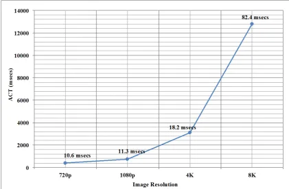
In Figure 6, the MSSED ACT and the corresponding standard deviation

(num-bers on the graph) for each image resolution are shown.

The ACT for MSSED is less than a second for images with resolution less than 1080 P. Even at this low resolution, only two frames can be processed in a second using the MSSED implementation. This high value of ACT makes the MSSED implementation unsuitable for real-time applications. The MSSED ACT is com-parable to that reported in the research work [3] by Heymann et al. In [3], the ACT for a 640 × 480 resolution image was 312 msecs compared to 401 msecs for a 1280 × 720 resolution image. Next, as the image resolution increases the ACT increases tremendously. The ACT of MSSED can be reduced further by using multiple cores of the Intel Xeon processor. It can be observed in Figure 6; the standard deviation is very less.

In Figure 7, the MPSSED ACT and the corresponding standard deviation for

each image resolution are shown. Based on the ACT, the MPSSED is capable of processing 720 p and 1080 p images in real time.

In Figure 8, the PSSED ACT and the corresponding standard deviation for

each image resolution are shown.

[image:21.595.113.535.400.676.2]

With PSSED implementation, the ACT is less than 16 msecs even with the 8 K-resolution image. This is comparable ACT of the convolution of 9 K-resolution images using GPUs, described in [40] to be 10 msecs. The low ACT would allow

(22)

[image:22.595.109.537.62.354.2]

Figure 7. MPSSED ACT with varying image resolutions.

[image:22.595.113.541.393.682.2]

(23)

processing of the 8 K resolution images at 60 fps making the PSSED implemen-tation suitable for real-time applications. In the research work [12] it has been shown with homogenous multi-core DSP implementation a processing rate of 45 fps of 640 × 480 resolution images is achievable.

In Figure 9, the speedup of PSSED over MSSED and MPSSED are shown. The

speedup is found to vary from 592× to 829× and 78× to 143× over MSSED and MPSSED respectively with increasing image resolutions. It is seen that the spee-dup increases initially and reaches saturation. This is due to the finite amount of memory and cores available on the GPU for concurrent execution. The opti-mized CUDA C PSSED implementation performance is still significantly better compared to the Matlab based GPU implementation of the SSED.

The test image used for comparing performance is shown in Figure 10, and the corresponding final DoG image by PSSED is shown in Figure 11. Identical DoG images are created by the MSSED, MPSSED and PSSED.

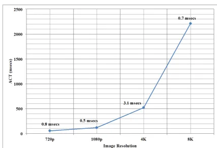
6.2. Phase 2

[image:23.595.116.535.385.673.2]

The ACT of PSIFT algorithm and its speed up w.r.t. sequential (SWS) Matlab SIFT (SSIFT) is provided in Figure 12. The ACT for a 720 p image is nearly 2.5 msecs making SIFT a feasible algorithm for real time applications. However, the ACT increases non-linearly with an increase in image resolution. The number of

(24)

[image:24.595.214.534.68.250.2] [image:24.595.216.535.277.465.2]

Figure 10. Test image.

Figure 11. Final image obtained from PSSED.

image points increases with increasing image resolution causing code to execute a block of points sequentially instead of parallel execution due to the unavaila-bility of idle SMs. Therefore, it reduces the speed up w.r.t. SSIFT. The speed up of PSIFT over SSIFT shown in Figure 12 is only for a set of 4 images of different resolutions. A change in an image, leads to a change in CKs and keypoints, leading to different workload.

Figure 13 shows the impact of keypoints on PSIFT’s performance for 720 p

(25)

[image:25.595.115.537.62.355.2]

Figure 12. PSIFT performance with varying image resolutions.

[image:25.595.114.537.394.685.2]

(26)

As mentioned before, phase 2 provides performance results of PSIFT tuned for faster execution. This performance boost is achieved by lowering the accura-cy of the SIFT algorithm. Figure 14 shows the accuracy of PSIFT in terms of the percentage of matching keypoints generated in comparison to SSIFT, which is adopted from Lowe’s algorithm. Figure 14 shows steep decrease in accuracy with an increase in performance. However, 89% keypoints matching SSIFT for 8 k images is an acceptable number of keypoints.

6.3. Phase 3

Since the accuracy of results are lower in phase 2, it is necessary to compare PSIFT optimized for ACT and PSIFT tuned for 100% accuracy. Figure 15 pro-vides the SWS for the two approaches. It is evident that tuning PSIFT for accu-racy does not scale well for higher resolution.

Figure 16 provides the SIFT descriptors generated for image. The figure

shows a number of keypoints are generated as an output for the SIFT algorithm. It matches with the keypoints generated by SSIFT, verifying the accuracy.

6.4. Phase 4

[image:26.595.115.537.399.680.2]

In this phase, our approach to select the number of threads is analyzed. The op-timal thread number for SSED is 256 threads. Figure 17 compares of perfor-mance of SIFT with optimal threads with threads lower and higher than optimal

(27)

[image:27.595.111.536.66.360.2]

Figure 15. PSIFT accuracy for various image resolutions.

[image:27.595.118.540.389.690.2]

(28)

[image:28.595.114.537.61.353.2]

Figure 17. Performance variation in PSIFT due to variation in threads.

values. It is seen that our approach provides the best performance of the five cases. Lower threads fail to hide memory latency and hence have worse perfor-mance. Higher threads hide memory latency as much as optimal case, but for higher data sizes requires more memory than optimal case. Hence performance deteriorates as seen in Figure 17.

(29)

[image:29.595.113.538.65.350.2]

Figure 18. PSIFT GPU resource utilization.

time, the MIPS are high while LCM is lower than 2% except for the initial load. This marks the SSED phase where data is pre-fetched by the compiler reducing LCM and increasing MIPS. During the data rearrangement phase, the MIPS are cut down by 50%. The LCM during this phase is observed to be between 0% - 15% indicating scattered memory access. This phase lasts till 85% of the execution time, followed by the keypoint localization and descriptor generation, which are similar to SSED. The plot shows that the GPU MIPS is high throughout the ex-ecution of the algorithm, indicating that our parallelization strategy is effective.

7. Conclusions and Future Work

(30)

and threads.

The performance of the parallelized SIFT thus obtained is presented, com-pared and analyzed. The following observations were made:

a) PSIFT performs better than the sequential and parallel Matlab implementa-tions.

b) Accuracy of the SIFT algorithm, in terms of number of keypoints generated, can be traded to obtain lower execution time.

c) PSIFT can process high-resolution images under 25 msecs when optimized for low execution time.

d) The number of keypoints in a given image has a significant impact on the execution time of PSIFT.

e) The implementation design phase strategies provided the optimal number of threads and blocks for PSIFT.

f) The two-phase parallelization strategies did show effective use of GPU re-sources.

Our approach to parallelization facilitates SIFT algorithm to be used for processing high-resolution images in real time. The future work would be to pro-vide a multi-GPU implementation.

References

[1] Lowe, D.G. (1999) Object Recognition from Local Scale-Invariant Features. The Proceedings of the Seventh IEEE International Conference on Computer Vision, 2, 1150-1157. https://doi.org/10.1109/ICCV.1999.790410

[2] Skrypnyk, I. and Lowe, D.G. (2004) Scene Modelling, Recognition and Tracking with Invariant Image Features. Third IEEE and ACM International Symposium on Mixed and Augmented Reality, 110-119. https://doi.org/10.1109/ISMAR.2004.53 [3] Heymann, S., Muller, K., Smolic, A., Frohlich, B. and Wiegand, T. (2007) SIFT

Im-plementation and Optimization for General-Purpose GPU. Proceedings of the In-ternational Conference in Central Europe on Computer Graphics, Visualization and Computer Vision, 144.

[4] Li, L.Y., Tong, X.H., Jin, Y.M., Chen, P., Liu, S.J. and Hong, Z.H. (2012) Bundle Adjustment of High Resolution Stereo Camera on Mars Express. Second Interna-tional Workshop onEarth Observation and Remote Sensing Applications, 243-245. https://doi.org/10.1109/EORSA.2012.6261174

[5] Yu, X.P., Liu, T., Li, P.X. and Huang, G.M. (2011) The Application of Improved SIFT Algorithm in High Resolution SAR Image Matching in Mountain Areas. In-ternational Symposium on Image and Data Fusion,1-4.

[6] Chen, K., Lin, C., Chiu, T., Chen, M. and Hung, Y. (2011) Multi-Resolution Design for Large-Scale and High-Resolution Monitoring. IEEE Transactions on Multime-dia, 13, 1256-1268. https://doi.org/10.1109/TMM.2011.2165055

[7] Turner, D., Lucieer, A. and Watson, C. (2012) An Automated Technique for Gene-rating Georectified Mosaics from Ultra-High Resolution Unmanned Aerial Vehicle (UAV) Imagery, Based on Structure from Motion (SfM) Point Clouds. Remote Sensing, 4, 1392-1410. https://doi.org/10.3390/rs4051392

(31)

of SIFT on Multi-Core Systems. IEEE International Symposium on Workload Cha-racterization, 14-23.

[9] Feng, L., Xu, T., Huang, Q., Wang, X. and Wang, P. (2010) SIFT Implementation Based on Parallel Computation. 6th International Conference on Wireless Commu-nications Networking and Mobile Computing, 1-4.

https://doi.org/10.1109/wicom.2010.5600662

[10] NVIDIA Developer Forum (2015). https://developer.nvidia.com/search/gss/SIFT [11] Warn, S., Emeneker, W. and Cothren, J. (2009) Accelerating SIFT on Parallel

Ar-chitectures. International Conference on Cluster Computing and Workshops. [12] Liu, X., Chen, W.J., Ma, T. and Xu, L.S. (2011) Real-Time Algorithm for Sift Based

on Distributed Shared Memory Architecture with Homogeneous Multi-Core dsp. 2nd International Conference on Intelligent Control and Information Processing, 2, 839-843. https://doi.org/10.1109/icicip.2011.6008366

[13] Yao, L., Feng, H., Zhu, Y., Jiang, Z., Zhao, D. and Feng, W. (2009) An Architecture of Optimised SIFT Feature Detection for an FPGA Implementation of an Image Matcher. International Conference on Field-Programmable Technology, 30-37. https://doi.org/10.1109/fpt.2009.5377651

[14] Kim, J., Park, E., Cui, X., Kim, H. and Gruver, W.A. (2009) A Fast Feature Extrac-tion in Object RecogniExtrac-tion Using Parallel Processing on CPU and GPU. IEEE In-ternational Conference on Systems, Man and Cybernetics, 3842-3847.

[15] Jiang, G., Zhang, G. and Zhang, D. (2010) A Distributed Dynamic Parallel Algo-rithm for SIFT Feature Extraction. 3rd International Symposium on Parallel Archi-tectures, Algorithms and Programming, 381-385.

https://doi.org/10.1109/PAAP.2010.58

[16] Kang, S.H., Lee, S.J. and Park, I.K. (2014) Parallelization and Optimization of Fea-ture Detection Algorithms on Embedded GPU. International Workshop on Ad-vanced Image Technology, 108, 164-167.

[17] Huang, M. and Lai, C. (2014) Parallelizing Computer Vision Algorithms on Acce-leration Technologies: A SIFT Case Study. IEEE China Summit & International Conference on Signal and Information Processing, 325-329.

[18] Fassold, H. and Rosner, J. (2015) A Real-Time GPU Implementation of the SIFT Algorithm for Large-Scale Video Analysis Tasks. SPIE/IS&T Electronic Imaging, International Society for Optics and Photonics.

[19] Mohammadi, M.S. and Rezaeian, M. (2014) Towards Affordable Computing: Sift-CU a Simple but Elegant GPU-Based Implementation of SIFT. International Journal of Computer Applications, 90.

[20] Marinelli, M., Mancini, A. and Zingaretti, P. (2014) GPU Acceleration of Feature Extraction and Matching Algorithms. IEEE/ASME 10th International Conference on Mechatronic and Embedded Systems and Applications, 1-6.

https://doi.org/10.1109/mesa.2014.6935620

[21] Kumar, R.P., Muknahallipatna, S.S. and McInroy, J.E. (2014) SIFT’s Scale-Space Extrema Detection on GPU for Real-Time Applications (WIP). Proceedings of the 2014 Summer Simulation Multiconference, 67.

[22] Brown, M. and Lowe, D.G. (2002) Invariant Features from Interest Point Groups. Proceedings of the British Machine Vision Conference, 1.

https://doi.org/10.5244/c.16.23

(32)

Parallel Computer: Applications to Computer Vision. Proceedings of the 17th In-ternational Conference on Pattern Recognition, 1, 805-808.

https://doi.org/10.1109/ICPR.2004.1334339

[24] NVIDIA, NVIDIA CUDA. http://www.nvidia.com/object/cuda_home_new.html [25] NVIDIA, NVIDIA CUDA C Programming Guide.

http://docs.nvidia.com/cuda/cuda-c-programming-guide

[26] Meng, J., Morozov, V.A., Vishwanath, V. and Kumaran, K. (2012) Dataflow-Driven GPU Performance Projection for Multi-Kernel Transformations. Proceedings of the International Conference on High Performance Computing, Networking, Storage and Analysis, 82.

[27] Zhang, Y. and Mueller, F. (2012) Auto-Generation and Auto-Tuning of 3D Stencil Codes on GPU Clusters. Proceedings of the Tenth International Symposium on Code Generation and Optimization, 155-164.

https://doi.org/10.1145/2259016.2259037

[28] Meng, J. and Skadron, K. (2011) A Performance Study for Iterative Stencil Loops on GPUs with Ghost Zone Optimizations. International Journal of Parallel Program-ming, 39, 115-142. https://doi.org/10.1007/s10766-010-0142-5

[29] Unat, D., Cai, X. and Baden, S.B. (2011) Mint: Realizing CUDA Performance in 3D Stencil Methods with Annotated C. Proceedings of the International Conference on Supercomputing, 214-224. https://doi.org/10.1145/1995896.1995932

[30] Maruyama, N., Sato, K., Nomura, T. and Matsuoka, S. (2011) Physis: An Implicitly Parallel Programming Model for Stencil Computations on Large-Scale GPU-Accele- rated Supercomputers. International Conference for High Performance Computing, Networking, Storage and Analysis, 1-12. https://doi.org/10.1145/2063384.2063398 [31] Stromme, A., Carlson, R. and Newhall, T. (2012) Chestnut: A Gpu Programming

Language for Non-Experts. Proceedings of the 2012 International Workshop on Programming Models and Applications for Multicores and Manycores, 156-167. https://doi.org/10.1145/2141702.2141720

[32] Nugteren, C. and Corporaal, H. (2012) Introducing “Bones”: A Parallelizing Source- to-Source Compiler Based on Algorithmic Skeletons. Proceedings of the 5th Annual Workshop on General Purpose Processing with Graphics Processing Units, 1-10. https://doi.org/10.1145/2159430.2159431

[33] Verdoolaege, S., Carlos Juega, J., Cohen, A., Ignacio Gómez, J., Tenllado, C. and Catthoor, F. (2013) Polyhedral Parallel Code Generation for CUDA. ACM Transac-tions on Architecture and Code Optimization, 9, 54.

https://doi.org/10.1145/2400682.2400713

[34] Brodtkorb, A.R., Hagen, T.R. and Sætra, M.L. (2013) Graphics Processing Unit (GPU) Programming Strategies and Trends in GPU Computing. Journal of Parallel and Distributed Computing, 73, 4-13. https://doi.org/10.1016/j.jpdc.2012.04.003 [35] Liu, L., Li, Z. and Sameh, A.H. (2008) Analyzing Memory Access Intensity in

Paral-lel Programs on Multicore. Proceedings of the 22nd Annual International Confe-rence on Supercomputing, 359-367. https://doi.org/10.1145/1375527.1375579 [36] Ryoo, S., Rodrigues, C.I., Baghsorkhi, S.S., Stone, S.S., Kirk, D.B. and Hwu, W.M.W.

(2008) Optimization Principles and Application Performance Evaluation of a Mul-tithreaded GPU Using CUDA. Proceedings of the 13th ACM SIGPLAN Symposium on Principles and Practice of Parallel Programming, 73-82.

(33)

[37] Volkov, V. (2010) Better Performance at Lower Occupancy. Proceedings of the GPU Technology Conference, 10, 16.

[38] Iandola, F.N., Sheffield, D., Anderson, M.J., Phothilimthana, P.M. and Keutzer, K. (2013) Communication-Minimizing 2D Convolution in GPU Registers. IEEE In-ternational Conference on Image Processing, 2116-2120.

https://doi.org/10.1109/icip.2013.6738436 [39] Papi. http://icl.cs.utk.edu/papi/

[40] Vedaldi, A. (2007) An Open Implementation of the SIFT Detector and Descriptor. UCLA CSD.

Submit or recommend next manuscript to SCIRP and we will provide best service for you:

Accepting pre-submission inquiries through Email, Facebook, LinkedIn, Twitter, etc. A wide selection of journals (inclusive of 9 subjects, more than 200 journals)

Providing 24-hour high-quality service User-friendly online submission system Fair and swift peer-review system

Efficient typesetting and proofreading procedure

Display of the result of downloads and visits, as well as the number of cited articles Maximum dissemination of your research work