A TECHNIQUE FOR TUMOR REGION IDENTIFICATION USING CELLULAR NEURAL NETWORK

DATA CLASSIFICATION BY SAC “SCOUT ANTS FOR

CLUSTERING” ALGORITHM

1_{MOHAMED HAMLICH,} 2_{MOHAMMEDRAMDANI}

12 _{Computer science labs, of FSTM, UH2}

E-mail:[email protected], [email protected]

ABSTRACT

In this paper, we propose a new learning method for clustering heterogeneous data with continuous class. This method in a first step finds the optimal path between the data using ant colony algorithms. The distance adopted in our optimization method takes into account all types of data. In the second step, instances in the optimal path, are divided into homogeneous groups. A new criterion for the separation of clusters is used; it is based on transition probabilities between the instances. A third step is to find the

prototype of each cluster to identify the cluster membership of any new data injected. After applying a

clustering algorithm, we want to know whether the cluster structure found is valid or not. To validate our approach, we have applied our method on different types of artificial data and real data from UCI Machine Learning Repository. The results obtained showed an obvious improvement of validation indexes compared to those of ACA, ACOC, k-means and KHM algorithms.

Keywords: Data clustering, Best path, Cluster prototype, Continuous class.

1. INTRODUCTION

The ant colony algorithms simulate the behavior of real ants using a colony of artificial ants to find the optimal path between the data [1]. The basic idea is that the probability that an ant chooses a point among all possible points is dependent on the amount of pheromone deposited by the ant and on the distance between the point of departure and arrival (refers to equation 1). To develop an efficient method of data aggregation, it is necessary to modify and adapt the concepts related to the actual life of ants, so they can be used effectively to solve data mining problems [5]. The motivation of this work is to develop methods based on ant colonies that can treat heterogeneous data with continuous class. We have developed the algorithm named Fuzzy Ant-Miner [12] that extracts fuzzy rules [9] from training data[2]. It processes data with nominal class and has the disadvantage of not treating the data with continuous class. We propose here a new method of data clustering based on the ant colonies algorithms [8]. This method divides the heterogeneous data, with continuous class into clusters. A cluster is therefore a collection of objects which are “similar” between them and are “dissimilar” to the objects belonging to other clusters.

In this paper we first describe the base Ant Colony Optimization algorithm (ACO) in section (2). In the third section, we explain the

improvements made by our clustering method. In the section (4), we present results obtained by our method, and we compare the results with other data clustering algorithms.

2. DATA CLUSTERING WITH ANT

COLONY OPTIMIZATION

The ant colony optimization algorithm (ACO), introduced by Dorigo [3], is a probabilistic technique which can be reduced to finding good paths through graphs. They are inspired by the behavior of ants in finding paths from the colony to food. ACO is an adaptative nature inspired algorithm concretely implemented, and applied in various areas.

The ACO algorithm, applied in data clustering is generally processed in two steps [14]:

• The search for the shortest path between data.

• The separation of data into similar groups.

2.1Searching optimal path

The objective of the first step is to find a good path connecting all the points in the dataset using the ACO algorithm [4]. This is equivalent to the construction of a graph whose nodes constitute the data set analyzed. The probability that the ant k,

which occupies the position i, moves to the next

[ ] [ ]

[

] [ ]

. ) ( . ) ( ) ( ∑ = Ζ ∈ k

k ik ik ij ij k ij t t t

P _{α β}

β α η τ η τ Where :

• Zk is a list of data not visited by ant k.

• τij(t) Represents the amount of

pheromone in the transition between data i

and j.

• α is the intensity level of pheromone.

• β is the visibility of the data.

• ηij is the inverse of the distance between i

and j data.

Once the ants have completed their paths, the levels of pheromone, in the transitions evaporate and a new pheromone amount is deposited between each pair of data. It depends on the quality of the solution built (path length). In practice, in order to update pheromone level, we use the formula (2) adapted to each data pair (i, j):

= +1) (t

ij

τ (1−ρ).τ_ij(t)+∆τ_ij(t)

(2)

• ρ∈[0,1] represents the decay coefficient of

the level of pheromone.

• ∆τij(t)is the increment pheromone added

between data (i, j).

The formula giving the increment pheromone

added in the transition between the two data (i, j) is

as follows [8]:

) ( ) , ( 0 ) ( ) , ( ) ( ) ( t T j i pour t T j i pour t L n t K K K k ij ∉ ∈    =

∆τ

(3)

Where:

• LK(t) : The path length constructed by

the ant k.

• TK(t) : The set of pairs of data belonging

to a path constructed by ant k.

• n: The number of data.

The illustration of this first step, which is to find the good path, is shown in Figure 4.

2.2 Data clustering

The objective of the next step is to separate data into homogeneous groups. Clustering [15] is the act of cutting a set of objects into groups (clusters) so that the characteristics of objects in the same cluster are similar and that the characteristics of objects in different clusters are distinct.

The method [16] starts with the first instance of the best path found in the first step. The vector representing this data of the sequence is recognized

as a center of gravity “µbefore” of the first group to be

separated. The following data is added to the first

group and the new gravity center “μafter” is

calculated. The method calculates the cohesion [14] of the first group using the whole similarity measure, in which the gravity center vector represents the considered group. If the change of cohesion has an acceptable value (refer to equation 4), the element considered becomes a permanent member of the group; otherwise it will be considered as the first element of a new group. The method then tries to expand the group further by adding the following element of the sequence.

(

)

2 2 2 δ µ µ µ − < − before before after Where:

δ : attachment coefficient between 0 and 1. μafter, μbefor: the gravity centers after and before adding a data to the group.

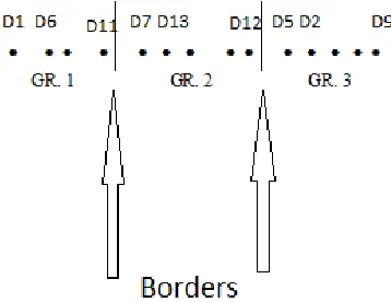
The separating of groups (Gri , i = 1 to 3) is

shown in Figure 1. If a group consists of a single data then this one will be assigned to the closest group.

During processing, each group is represented by a center of gravity. The number of separate groups is highly dependent of attachment coefficient. If the parameter δ is large (close to 1), then we obtain many groups with a high degree of cohesion as a result of treatment. A low value of δ gives us little groups with less cohesion.

Figure 1: Illustration Of Data Clustering

The main objective of our approach is to overcome these limitations while retaining the benefits of clustering algorithms based on ant colony optimization.

3. IMPROVEMENTS BY OUR METHOD

3.1 Clustering criteria

In our method, we introduced a new criterion to divide the data into homogeneous groups. This criterion is based on the transition probabilities already calculated in the first step. The method searches the lower transition probability in the best path found. If it satisfies the condition (5), then a boundary between the positions i and j is marked.

ij

P

<

ε

(5)

Where:

• ε is a parameter called the coefficient of

attachment and its range is [0, 1].

• Pij is the probability of transition between

instances i and j.

This criterion is based on the transition probabilities that take into account the distances and levels of pheromone. The processing time of the separation of groups will be smaller; indeed the transition probabilities have been already calculated in the first step.

3.2 Distance measure between heterogeneous data

Once the groups are formed, the method determines a representative prototype of each cluster. The prototype of a cluster is the one closest to all data of the cluster.

Suppose that the data set is defined by a number p

of attributes kinds. The position of each variable,

describing data objects is denoted by f and is from 1

to p. The distance dij [13] between instances i and j

in the sets of attributes f is given by the equation

(6).

Where

• (f)

ij

δ : Missing value (δ = 0) or present

value (δ = 1) indicator in attribute f.

• (f)

ij

d : Distance between positions i and j,

calculated according to its type.

3.3 Scout Ants for Clustering algorithm (SAC)

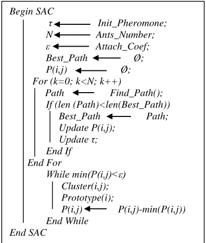
The pseudo-code below (refer to figure 2) shows the different processing stages of our method. The first loop (For) finds a good trajectory based on transition probabilities (refer to equation 1). The second loop (While) partitions data into homogeneous groups, based on the criterion (5). For each group, the method determines the most representative element; this prototype is one that looks at all the data in the cluster.

Figure 2: Pseudo Code Of SAC Algorithm.

3.3 The experiments on artificial data 3.3.1 Convexes data

We propose a set of artificial data (refer to table 1) to test our method. It consists of 37 instances that reflect the behaviors and outcomes of students. Each instance consists of a nominal attribute (Participation) and two continuous attributes (Absence and Note). The purpose of this experiment is to show that our method effectively separates clearly different clusters.

The initial values chosen are: 25 . 0 ) 0 ( = ij τ 1 = =β α 09 . 0 = ε Ants number=10

Initially, the first ant starts its journey from any

position i. Our method calculates all dij distance

between the points i and j. Then, calculates the

probability Pij to move from a starting point to the

destination j , taking into account the amount of

pheromone in the transition. This move will be (6) 1 ) ( 1 ) ( ) ( ∑ ∑ = = = p f f ij p f f ij f ij ij d d δ δ Begin SAC

τ Init_Pheromone; N Ants_Number; ε Attach_Coef; Best_Path Ø; P(i,j) Ø; For (k=0; k<N; k++)

Path Find_Path();

If (len (Path)<len(Best_Path)) Best_Path Path;

Update P(i,j); Update τ; End If End For While min(P(i,j)<ε) Cluster(i,j); Prototype(i);

P(i,j) P(i,j)-min(P(i,j)) End While

End SAC

effective to the given j if Pij is the greatest of all the

probabilities.

Suppose that the ant is in position 36, the P36 j(j=1

to 37) probabilities to transit to a position j are calculated and compared. If the greatest probability is P36 18, ant will move to position 18. Arriving at

this point, the ant will move to another position j

unexplored as P18 jis maximum (for our example, j

= 19) and thus on. The journey of the ant fig. 4 will

be completed when it will travel all data. The method is updating pheromone levels and a new ant begins a new journey.

The number of ants is entered by the user, but if there is a convergence towards a path then the method exits the loop before reaching the number of ants.

Table 1: Artificial Data.

Data Absence Participation Note

D0 4.5 non 4

D1 0 oui 16

D2 3 non 8

D3 0 oui 15.5

D4 0 oui 15

D5 0.5 oui 15.5

D6 2 oui 13

D7 0 oui 17

D8 0 oui 15.5

D9 3 non 9

D10 0 oui 17.5

D11 0 oui 18.5

D12 1.5 oui 12

D13 0.5 oui 16.5

D14 0 oui 16

D15 1 oui 15

D16 2.5 non 9

D17 1 oui 13.5

D18 7 non 4

D19 6 non 5

D20 12 non 2

D21 0 oui 17

D22 0 oui 15

D23 0 oui 16.5

D24 0 oui 15.5

D25 1 oui 14

D26 0 oui 18

D27 0.5 oui 15

D28 0 oui 17

D29 0 oui 17.25

D30 0 oui 17.5

D31 0 oui 15.5

D32 0 oui 16

D33 5 non 6

D34 1 oui 16

D35 0.5 oui 17

D36 7 non 3

Figure 3: Best Path Found By Ants.

The sequence of positions obtained in the best path refer to figure 4) is the following:

36, 18, 19, 33, 0, 2, 9, 16, 20, 12, 6, 17, 25, 15, 27, 5, 3, 8, 24, 31, 1, 14, 32, 23, 7, 21, 28, 10, 30, 26, 11, 29, 35, 13, 34, 4, 22.

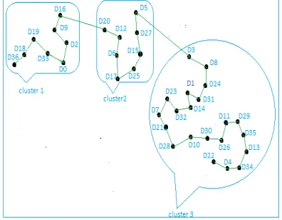
To cluster these data into homogeneous groups, the method compares the transition probabilities of the optimal path found. The minimum probability is considered as the first frontier between two groups. If a cluster contains only one instance, then it will be assigned to the nearest cluster.

Each cluster is represented by its prototype; this element is closest to all instances in the cluster. The values of the transition probabilities that justify the

relation (23) are P16 20 and P5 3. So the first

boundary is between positions 16 and 20, the second boundary is between positions 5 and 3. The illustration of data clustering in our example is shown in Figure 4.

Figure 4: Data Clustering

We note that our method automatically

Table 2: Prototypes Clusters

Cluster Prototype Absence Participation Note

1 D33 5 non 6

2 D20 12 non 2

3 D29 0 oui 17.25

The results are consistent and show that the number of hours absent students directly affects their results. More the number of ants is high over the method converges to a single optimal path. The number of clusters depends on attachment factor for a given optimal path.

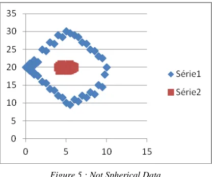
3.3.2 Not convexes data

We propose a set of artificial data distributed according to the diagram in the figure 5.

Figure 5 : Not Spherical Data

The classical clustering methods cannot separate

correctly this type of data.

Our method successfully separates the data into two clusters. In fact, the ant starts its journey from any point belonging to a given group. She will not leave this group as it has not explored all the points because it will always find a point in the same group closer than any point in the other group. Once she has explored all instances of the first group, it will pass to the other group with the lowest probability (border separating the two groups) transition. This probability justify the criterion (5), and the method marks a boundary in the transition.

3.4 The experiments on artificial data

To confirm the results obtained by our method, a

comparative study was done on real data. In this study, we conducted tests on standard databases,

obtained from the data warehouse UCI Learning

Machine Repository [11]. The characteristics of these databases are summarized in the table 3. The algorithms based on ant colonies deal with homogeneous data sets. To compare our method with these algorithms, we were forced to experiment on data sets whose attributes are of the same type. We first start by comparing our method with algorithms ACOC "Ant Colony Optimization Clustering algorithm" and KHM "k-Harmonic Means clustering algorithm" [19] on the datasets "Nursery" and "Solar Flare". Then we compare our method with algorithms ACA "Ant Clustering Algorithm" and k-means on the datasets "Iris", "Ionosphere", "Pima" and "Wine" [17], [18]. To validate and compare our clustering method, we measured indices of external and internal validation (Entropy, F-measure, and SSE (Sum Squared Errors)).

3.4.1 Comparison of algorithms SAC, ACOC

and KHM

For different number of ants, we set the attachment

coefficient ε to obtain different number of clusters.

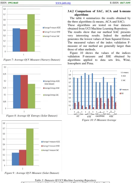
The results are summarized in the table 5. It show that the clustering given by the SAC method has the lowest entropy, and the largest F-measure, mean values.

On the other hand, we note that the best results of the SAC algorithm are those containing 4 and 5 clusters. This can be explained by the fact that we approach the real class’s number of the datasets. Figures 6 and 7 show, respectively, the mean values of the validation indexes: Entropy and

F-measure for dataset Nursery.

Figures 8 and 9 show, respectively, the mean values of the validation indexes: Entropy and

F-measure for dataset Solar Flare.

Figure 7: Average Of F-Measure (Nursery Dataset)

Figure 8: Average Of Entropy (Solar Dataset)

Figure 9 : Average Of F-Measure (Solar Dataset)

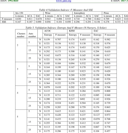
3.4.2 Comparison of SAC, ACA and k-means algorithms

The table 4 summarizes the results obtained by the three algorithms (k-means, ACA and SAC). These algorithms are tested on four datasets obtained from UCI Machine Learning Repository. The results show that our method SAC presents very interesting results. Indeed the method generates the lowest values of Sum Squared Errors. The measured values of the index validation F-measure of our method are generally larger than those of other methods.

Figure 10 shows the values of the indices validation F-measure and SSE obtained by algorithms applied to data sets Iris, Wine, Ionosphere and Pima.

Figure 10: F-Measure Average

Table 3: Datasets Of UCI Machine Learning Repository

Datasets Iris Ionosphere Pima Wine Nursery Solare Flare

Specifications

Instances 150 351 768 178 12960 1389

Attributes 4 34 8 13 8 10

Table 4:Validation Indexes: F-Measure And SSE

Iris 150 Wine Ionosphere Pima

k-means ACA SAC k-means ACA SAC k-means ACA SAC k-means ACA SAC

F-measure 0.830 0.811 O.870 0.943 0.896 0.935 0.710 0.700 O.842 0.709 0.623 O.821

SSE 0.167 0.187 0.090 0.056 0.101 0.050 0.296 0.291 0.156 0.278 0.331 0.179

Table 5. Validation Indexes: Entropy And F-Mesure (N:Nursery, S:Solar)

Clusters number

Ants number

ACOC KHM SAC

Entropy F-measure Entropy F-measure Entropy F-measure

2

5

N 0.159 0.707 0.174 0.453 0.162 0.582

S 0.321 0.136 0.312 0.138 0.318 0.576

15

N 0.173 0.124 0.174 0.453 0.170 0.625

S 0.292 0.173 0.300 0.141 0.294 0.610

25

N 0.162 0.675 0.316 0.165 0.160 0.517

S 0.321 0.136 0.265 0.139 0.270 0.541

3

5

N 0.105 0.104 0.094 0.532 0.100 0.679

S 0.164 0.199 0.167 0.170 0.148 0.612

15

N 0.183 0.180 0.163 0.923 0.170 0.620

S 0.285 0.344 0.289 0.295 0.158 0.598

25

N 0.162 0.180 0.166 0.535 0.160 0.526

S 0.364 0.222 0.270 0.231 0.186 0.670

4

5

N 0.078 0.410 0.202 0.225 0.100 0.768

S 0.115 0.126 0.125 0.284 O.070 0.800

15

N 0.135 0.711 0.122 0.152 0.085 0.940

S 0.200 0.219 0.217 0492 0.142 0.926

25

N 0.174 0.918 0.451 0.504 0.165 0.739

S 0.258 0.283 0.280 0.759 0.176 0.863

5

5 N 0.133 0.615 0.113 0.621 0.095 0.864

S 0.173 0.420 0.123 0.237 O.127 0.973

15

N 0.141 0.433 0.142 0.283 O.078 0.768

S 0.255 0.384 0.392 0.412 0.145 0.747

25

N 0.113 0.195 0.198 0.195 0.067 0.778

S 0.175 0.286 0.175 0.243 0.104 0.457

4. CONCLUSION:

In this paper, we propose a learning method

based on ant colonies to handle datasets with continuous class. Our method takes into account the attributes of continuous, nominal or ordinal type in the process of data clustering. In the process of separating the groups, we used a new probabilistic criterion. This criterion is based on the transition probabilities already calculated in the step of searching the best path between all instances.

We have shown in this paper that our method detects clusters of varied forms. The results on

real data are very encouraging, and far exceed other methods.

We intend to improve our SAC method by using the concepts of fuzzy logic to separate the data into homogeneous groups.

REFRENCES:

[1] G,A.Chan ,and A.Freitas, “A new classification-rule pruning procedure for an ant colony algorithm”, Lecture Notes in Artificial Intelligence 2005, 3871 25–36. [2] P.Clark, and T.Niblett, “The CN2 rule

[3] M.Dorigo,and T.Stutzle, “Ant Colony Optimization”, MIT Press, 2004.

[4] A.Freitas, R.Parpinelli, and H.Lopes, “Ant colony algorithms for data mining”, Sci. & Tech. 2nd Ed, 2008.

[5] H.Liu, F.Hussain, C.Tan, and M.Dash, “Discretization: An enabling technique”, Data Mining and Knowledge Discovery 2002, 6 393–423.

[6] D.Martens, M.Backer, R.Haesen, J.Vanthienen, M.Snoeck, and B.Baesens,

“Classification with ant colony

optimization”, IEEE Transactions on Evolutionary Computation 2007, 11(5) 651– 665.

[7] F.Otero, A.Freitas, and C.G.Johnson, “cAnt-Miner: an ant colony classification algorithm to cope with continuous attributes, in Ant Colony Optimization and Swarm Intelligence”, LNCS 5217, 2008 Springer, pp. 48–59.

[8] R.Parpinelli, H.Lopes, and A.Freitas, “Data mining with an ant colony optimization

algorithm,” IEEE. Transactions on

Evolutionary Computation, 2002, vol. 6, no. 4, pp. 321–332.

[9] M.Ramdani, « Système d’induction formelle à base de connaissances imprécises », Thèse de doctorat, Université Paris 6, 1994.

[10] M.Hamlich,and M.Ramdani, “Fuzzy classification method by ant colonies”,

International Conference on Discrete

Mathematics & Computer Science DIMACOS’11, 2011, pp. 69.

[11] UCI Machine learning Repository,

http://archive.ics.uci.edu/ml/datasets.html. [12] M.Hamlich,and M.Ramdani, “Data

classification by Fuzzy Ant-Miner”, IJCSI International Journal of Computer Sciences issues, Vol 9, Issue 2, N° 3, Marsh 2012, ISSN (Online) 1694-08 14.

[13] S.Pinjuši´c ´Curi´c and M.Vrani´c and

D.Pintar, Improvement of Hierarchical

Clustering Results by Refinement of Variable Types and Distance Measures. ATKAFF 52(4), 353–364(2011).

[14] ŁUKASZ MACHNIK, « A document

clustering method based on ant algorithms”,

Task Quarterly 11 No 1–2, 87–102, revised

manuscript received 22 January 2007

[15] RUI XU and DONALD C. WUNSCH, II, “Clustering”, Published by John Wiley & Sons, Inc., Hoboken, New Jersey, 2009 by Institute of Electrical and Electronics Engineers, Library of Congress Cataloging-in-Publication Data is available. ISBN: 978-0-470-27680-8.

[16] M.Hamlich, and M.Ramdani, «Improved ant colony algorithms for data classification », Complex Systems (ICCS), 2012, Agadir, ISBN: 978-1-4673-4764-8.

[17] U.Boryczka, “Ant Clustering Algorithm”, Intelligent Information Systems 2008, ISBN 978-83-60434-44-4, pages 377-386

[18] U.Boryczka, “Ant colony metaphor in a new

clustering algorithm” , Control and

Cybernetics, Vol. 39 (2010) No. 2

[19] M.Divyavani, T.Amudha, “Comparing the Clustering Efficiency of ACO and K-Harmonic Means Techniques, International Journal of Computer Science. Engineering and Applications (IJCSEA) Vol. 1, No. 4, August 2011.

[20] R.Priya Vaijayanthi, A. M. Natarajan, J.Raja