SOLVING ECONOMIC DISPATCH PROBLEM USING PARTICLE SWARM OPTIMIZATION BY AN EVOLUTIONARY TECHNIQUE FOR INITIALIZING PARTICLES

659

A METHOD OF AGRICULTURAL AREAS SAR DATA

SEGMENTATION BASED ON UNSUPERVISED

FULL-POLARIMETRIC

HONGFU WANG, XIAORONG XUE

School of Computer and Information Engineering, Anyang Normal University, Anyang 455000, Henan,

China

ABSTRACT

Classification is achieved by Markov random field filtering on the original data. The result is a series of segmented maps, which differ in the number of (unsupervised) classes. For a (compatible) supervised approach, only the first and last step have to be applied. Results are discussed for the agricultural areas Flevoland in The Netherlands (AirSAR data)and DEMMIN in Germany, using the NASA/JPL AirSAR system and the DLR ESAR system, respectively. The applications include the use of groundtruth for legend development, the check for ground truth completeness, and the construction of a bottom-up hierarchy of the characteristics that can be distinguished in the radar data. The latter gives important insights in physics of polarimetric radar backscattering mechanisms.

Keywords: Unsupervised Classification, Agricultures, Data Segmentation, Full Polarimetric

1. INTRODUCTION

Versatile, robust and computational efficient methods for radar image segmentation, which preserve the full polarimetric information content, are of importance as research tools, as well as for practical applications in land surface monitoring.

In this paper, the utility of a full-polarimetric unsupervised classification approach will be evaluated using airborne radar data collected in the growing season at two agricultural test sites in Europe. The first is the Flevoland site located in The Netherlands. During the 1991 MAC Europe campaign C-,L-(and P-)band polarimetric data were collected by the NASA/JPL AirSAR system[3].The other is the DEMMIN(Durable Environmental

Multidisciplinary Monitoring Information

Network)area in Northern Germany. Here L-band ESAR data were collected during the ESA/DLR AGRISAR 2006 campaign [7].For practical

application, multitemporal sampling schemes

should be developed to obtain high classification accuracies in the early or mid-stages of the growing season.

Using seven polarizations: HH, HV,VV, RR, RL, 45C, and 45X , and all three frequency bands, a classification accuracy level of 70.5% is achieved for3 3 pixel aggregates and a level of 90.5% on a per-field basis. In [4], the use of optimal polarization selection and a wavelet-based texture

feature set is discussed. For 13 classes, including water, using three frequency bands and three synthesized optimized polarizations an accuracy of 91.1% is achieved. In [13], applying a dynamic learning neural network, the accuracy increases to 95.4%. However, for C-band only, the result reduces to 67.9% and for L-band to 73.1%. In [5], the use of the complex Wishart distribution for the covariance matrix and the use of Maximum Likelihood classifiers, for different polarization combinations, are discussed. For 11 classes, including water, the best single band case is L-band fully polarimetric with 81.6%, while C-band achieves 66.5%. Using all three bands a level of 91.2% is reached.

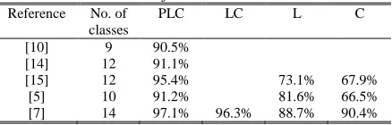
Using pixel aggregates and Maximum Likelihood classifiers better results are obtained for all band combinations, notably for the C-band. A summary is given in Table I. An objective comparison is not possible since none of the methods is optimized or complete for mapping yet and different evaluation methods may have been used.

Table I : Comparison Of Best Single Observation Date Classification Results

Reference No. of

classes

PLC LC L C

[10] 9 90.5%

[14] 12 91.1%

[15] 12 95.4% 73.1% 67.9%

[5] 10 91.2% 81.6% 66.5%

660

2.

A

D

In the meantime, piracy becomes increasingly rampant as the customers can easily duplicate and redistribute the received multimedia content to a large audience. [5].

The overall unsupervised approach consists of six processing steps. It is noted that this approach allows study of fully polarimetric data (using the 9-intensities representation), as well as single, dual or triple polarization (described by 1, 2, or 3 intensities, respectively) and forms of partial polarimetric data (described with 4–8 intensities). Moreover, multitemporal and/or multiband data sets can be studied.

When using only two of these six processing steps (viz. Steps 1 and 5)it is possible to make a

supervised(full-polarimetric)classification. Since

identical algorithms are applied it allows for a fair comparison between these two fundamentally different approaches. It is also possible to replace (a certain fraction of) unsupervised cluster statistics by supervised class statistics. This hybrid approach allows utilization of the strong points of both techniques in an elegant way.

2.1 Polarimetric Transform (Step 1)

Fully polarimetric target properties for uniform distributed scatterers can be described with nine independent real numbers. For the covariance matrix a Hermitian matrix, these properties are contained in the three real numbers on the diagonal and the six real and imaginary parts of the three complex numbers above the diagonal.

hh hh hh hh hh vv

hv hh hv hv hv vv

vv hh vv hv vv vv

S S S S S S

C S S S S S S

S S S S S S

∗ ∗ ∗ ∗ ∗ ∗ ∗ ∗ ∗       =_{ }       (1)

According [7], it is possible to describe the full

polarimetric information content with nine

intensities, for example as

(2)

where the subscripts of σ0denote the receive and

transmit polarizations of the three common polarization bases: horizontal(h), vertical(v) , left circular(l) , right circular(r) , 45 linear( +or +45) and -450 ; linear ( -or -45).

Statistical properties of the polarimetric

backscatter behavior for a single homogeneous area are described by the complex Wishart distribution. However, these distributions don’t necessarily well describe the statistics for pixels located in separate homogeneous areas of the same class because of between-field variation in, for example, biophysical parameters.

2.

and 4)

Unsupervised data clustering is performed in a sequence of three steps: segmentation followed by hierarchical clustering and partitional clustering.

Step 2 (Segmentation): The intention of this step is preparation for hierarchical clustering (in Step 3). Segmentation is used to convert the image pixels into a (large) number of segments (homogeneous regions). Identifying the optimal number of segments is not the goal of this step. Over-segmentation is allowed and even preferred since it provides more flexibility to form clusters in Step 3. However, it is not recommended to allow for too many small segments, e.g., close to singletons, because this may lead to computational problems in Step 3. Here, a region growing segmentation (RGS) algorithm is applied (on the masked image) to obtain homogeneous regions (H). RGS is a simple “average linkage” segmentation technique, which starts with a number of initial seed pixels, and creates homogeneous regions by grouping adjacent pixels to the current segment if the distance between an adjacent pixel and the mean of the current segment is below a certain threshold [6]. Region growing segmentation often creates a lot of segmented regions, but also leaves a large fraction of the image unsegmented. These unsegmented regions are usually small and may well contain noise, or small artefacts. These regions are not important for the estimation of cluster statistics or even disturb the calculations. Therefore, they are discarded until the final step 5.

Step 3 (Hierarchical Clustering): The Model-based Agglomerative Clustering (MAC) technique, a hierarchical model-based clustering approach [5], is selected for the next step. However, instead of starting to merge singleton clusters (pixels), the method starts with clusters (i.e., the homogeneous

0 0 0 45 0 4 5 0 0 0 4 5 0 0 4 5 R e I m R e I m R e I m

h h hh

h h h v h v

v v v v v v

hh v v

h h v v H

r r hh h v

h h h h v

h l

hv v v l

h v v v S S S S S S

S S

S S B

661 regions H, obtained from Step 2. This method

makes hierarchical model based clustering

computational feasible for a large image. At each hierarchical merging step, the algorithm continues to join that pair of clusters (based on the “shortest” distance) which leads to the largest increase in classification likelihood. Effective implementation of this algorithm is proposed in [6]. At the end, a dendrogram results, presenting how cluster Pairs are joined. A range of selected models (defined and differentiated by the number of clusters) can be obtained by cutting the dendrogram at the appropriate levels.

Step 4 (Partitional Clustering): At this stage, the Expectation-Maximalization (EM) algorithm [12], [13] can be applied without difficulty using the estimated statistics for each selected model (instead of random initialization which may lead to clustering problems). With good initial statistics, the EM algorithm should convert very quickly to an optimal solution for each model. It is noted that Steps 3 and 4 are only applied to the pixels included in homogenous regions (segments) H, determined in Step2.

2.3 Classification and Legend Development

To extend classification to the entire image, a Markov Random Field (MRF) classification is performed using the class statistics obtained from Step 4. Since the MRF takes spatial information (from the pixel neighborhood) into account, using the previously established class statistics, the classification is very robust to outliers, noise and artifacts possibly present in other parts of the image.

Figure ure1 shows unsupervised classification results for the L- and C-band combination for the range of models with only 2, 3, 4, and 5 clusters, respectively.

(a)

(b)

(c)

(d)

Figure1: Flevoland Unsupervised Classification Results For The L- And C-Band Combination For Models

2–5. (A) Model 2, (B) Model 3, (C) Model 4, And (D) Model 5, With Two, Three, Four, And Five Classes,

Respectively.

3. TEST SITES AND DATA

A. Flevoland and 1991 AIRSAR Data

662

analysis presented in this paper a 640 ×640 pixel

sub-image with a 46.8–59.6 incidence angle range is used for which 182 fields are available(Table II).

B. DEMMIN and 2006 ESAR Data

The terrain of the DEMMIN area is fairly flat and sizes of agricultural fields are around 80 ha. Besides agricultural crops, the area comprises some villages and mixed and deciduous forests with high species diversity.

DLR’s ESAR system collected radar data at 16 flight-days spread regularly over a whole growing season, viz. the period April 18 until August 2, 2006 [8]. The AGRISAR ground data collection campaign targeted several fields yielding data like soil moisture, surface roughness, biomass (wet and dry) estimates, crop phenology and meteorological data [10].

Table II: Cover Types,Crop Identifiers(Labels)And Number Of Fields Of The 1991 Flevoland Ground Data

Set

Table III: Crop Types, Crop Identifiers (Labels), Total Area (In Ha), And Percentage Of Area Of The Fields Of

The Demmin 2006 Ground Data Set. Note: The Second Column Is The Legend For Figure2

Type Label Area (ha) Area (%)

Corn COR 39.1 5.6%

Rape RAP 149.2 21.3%

Field grass GR1 3.0 0.4%

Cutting pasture

GR2 13.6 1.9%

Set aside; rape

SAS 11.1 1.6%

Grassland GR3 2.5 0.4%

Winter barley

BAR 28.0 4.0%

Winter wheat

WHE 339.4 48.5%

Sugar beet SBT 32.4 4.6%

Forest FOR 44.1 6.3%

Urban area URB 37.5 5.4%

The crop type map comprises 11 crops (Table III).Some crops cover large fractions of the area Like winter wheat (48.5%) and rapeseed (21.3%). During classification analysis it became clear that several crop classes are hardly distinct. For example, the class” set-aside rapeseed” is the same as the class rapeseed, but sowed two weeks later. The three classes of grass are very similar (for the radar) for the period studied. The class urban is a mixture of build-up areas and gardens with trees. The latter resembles (for the radar) the forest class. To evaluate classification results the class set-aside rapeseed is considered to be the same as rapeseed, the grasses are put together into a single class, and the classes urban and forest may be put together.

4. RESULTS

A. Results for Flevoland

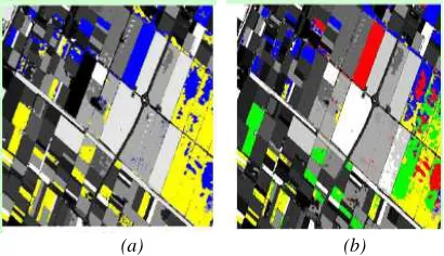
For Flevoland, a single date C-and L-band Polari metric image was analysed.Using the unsupervised approach introduced in Section II, a number of models can be generated for C-band, for L-band, or for the combination of C-and L-band. In Figure .2, results for the C-and L-band combination are shown for models 2 until 5.The model number equals the number of unsupervised classes in the image. In Figure2 (b), for example, the white fields are potato fields, while the black and gray fields are composite classes. Results for higher model numbers yield more (pure) classes, less composite classes, but also more sub-classes.

(a) (b) Figure2: Flevoland Unsupervised Classification Results For The C&L-Band Combination.Note:Top Of

Image Is The Near Range; Bottom Image Is The Far Range.

B.Results for DEMMIN

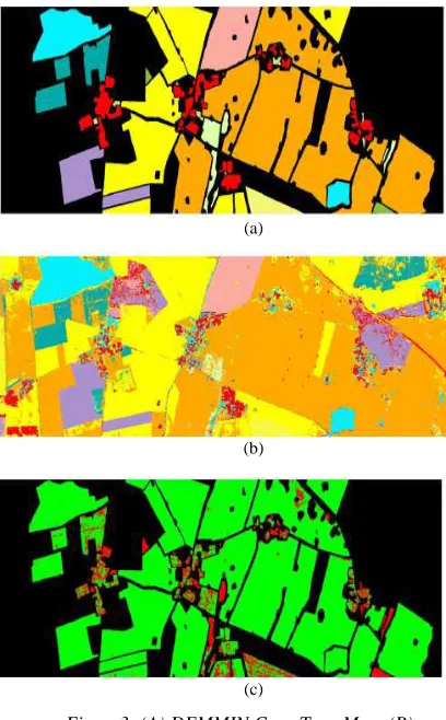
A straightforward supervised classification using three dates, three polarizations and the 11 classes of the crop type map has been conducted as a first analysis step. In Figure.3, these results can be evaluated by comparing the crop type map, the

Type Lab

el

Fields Type Label Fields

Barley BA

R

11 Onion

s

ONI 3

Beans BE

A

6 Peas PEA 3

Corn CO

R

7 Potato POT 42

Flax FLA 2 Rapes

eed

RAP 7

Fruit trees

FR U

1 Sugar

beet

SBT 32

Grasslan d

GR A

20 Wheat WHE 47

Lucerne LU

663 classified image and the error map. Set-aside rape classified as rape, and gardens (with trees)in the urban areas classified as forest, are considered as errors in Figure.3(c).There is also confusion

between the different classes of

grass.Nevertheless,the total classification result still is 93.1%.When aggregated to seven classes this result improves to 95.7%(Table V).The main remaining error is the classification of grass as wheat.

(a)

(b)

(c)

Figure3: (A) DEMMIN Crop Type Map, (B) Supervised Classification Of Multitemporal ESAR Images

Using Three Dates (June 3, July 5, And July 25, 2006) With Three Polarizations (HH, VV, And PL), (C) Error Map (Green: Correct; Red: False; Black: No Ground Truth). Note: Top Of Image Is The Near Range; Bottom

Of Image Is The Far Range.

The unsupervised classification of the same data set yields an entirely different result. The clustering reveals some 20 classes (in the area where ground truth is present) which can be aggregated to eight main classes as shown in Table III and Figure. 4.

Figure 4: Map Of DEMMIN Unsupervised Classification Results Aggregated Into Eight Classes.

5. CONCLUSION

The model for less estimated parameters, calculation of speed, can handle the trend change, price sequence multiple cycle, and the third order moment between torque ripple and the correlation with the load. PJM power market on June 1, 2007 to September 9th, 2010 the historical data analysis shows that the second order moment and system load square to electricity price average price have significant influence on the sequence, with weeks, half moon, bimonthly, season, monthly, such multiple cycle and second half, the torque ripple of agglomeration and the third order moment torque

displays obvious synchronous time-varying

characteristic.

A simple, robust, and very accurate data segmentation technique for unsupervised and supervised image classification has been introduced which can handle full-polarimetric data as well as

partial polarimetric data and multitemporal

observations. Basic elements of the approach are the transform of the polarimetric information content into nine intensities and the use of masks to derive unsupervised cluster statistics from selected areas only. Another strong feature of the algorithm is the preservation of line elements and very small objects (such as the corner reflectors). The unsupervised approach may be particularly useful to detect missing ground truth, or poorly representative ground truth, and can be used to support the development of map legends. For example, the technique, i.e. , a supervised and unsupervised hybrid approach, recently has been applied successfully to develop land cover type legends for a high resolution “wall-to-wall” map of the island Borneo, comprising as much as 544 ALOS PALSAR Fine Beam single and dual-polarization images [10].

664 proposed in literature. Moreover, such trees may generate important insight in the scattering mechanisms. The relative importance of crop differences, (full-polarimetric) incidence angle effects and sub-classes (related to factors such as crop varieties or row direction) may be assessed.

The overall classification results range between 84.3% and 98.0%, depending on number of observations dates and radar band(s) used, with higher values for the supervised approach, and

substantially more thematic detail for the

unsupervised approach. The unsupervised approach may be used to derive suitable training sets for the supervised approach which is much easier to apply on large scale.

For practical application, the accuracy of mapping should be in excess of approximately 90% (to be competitive with or complementary to ground survey), and provide sufficient thematic detail on (the main) crop types and, possibly, on differences in crop development. The results presented here suggest this is feasible using polarimetric data of one or more frequency bands, collected at one or more dates. More study is needed to determine optimal sampling schemes, and optimal polarization combinations. Good results may also be obtained by dense time series of single or dual-polarization data. In any case, the approach presented here is useful and sufficiently versatile to support such studies.

For space borne data, the number of independent radar looks per unit area is much lower, and application may be limited to sufficiently large fields. For operational crop monitoring systems (larger) time series of dual-polarization data may be

preferred. The RADARSAT-2 and future

SENTINEL-1 systems are of particular interest.

ACKNOWLEDGEMENTS

This work was supported the Project of National Natural Science Foundation of China (U1204402).

REFERENCES:

[1] S. N. Anfinsen, A. P. Doulgeris, T. Eltoft, “Estimation of the equiva-lent number of looks in polarimetric synthetic aperture radar imagery”

IEEE Trans. Geosci. Remote Sens., Vol.47,

No.11, 2009, pp.3795–3809.

[2] J. Amores, N. Sebe, P. Radeva, “Boosting the distance estimation application to the K-nearest neighbor classifier”, Pattern Recogn. Lett., Vol.27, No. 3, 2006, pp.201–209.

[3] J. B. Bordes et al., “Semantic annotation of

satellite images”, Proceedings of Fifth

Int.Conf.on Machine Learning and Data Mining in Pattern Recognition, 2007, pp.120–133.

[4] R. Meir, G. Ratsch, “An introduction to boosting and leveraging”, Adv. Lect. Mach.

Learn., 2003, pp.119–184.

[5] D. H. Hoekman and M. A. M. Vissers, “A new polarimetric classification approach evaluated

for agricultural crops”, IEEE Trans.

Geosci.Remote Sens., Vol. 41, No. 12, 2003, pp.

2881–2889.

[6] B. R. Corner, R. M. Narayanan, and S. E. Reichenbach, “Noiseestimationin remote sensing imagery using data masking”, Int. J. Remote

Sens., Vol.24, No.4, 2003, pp.689–702.

[7]K.S.Sim and N.S.Kamel, “Image signal-to-noise ratio estimation using the autoregressive model”,

Scanning, Vol.26, No.3, 2004, pp.135-139.

[8] M. E. Mejail, J. JacoboBerlles, A. C. Frery, O. H. Bustos, “Classification of SAR images using a general and tractable multiplicative model”,

Int. J. Remote Sens., Vol.24, No.18, 2003,

pp.3565–3582.

[9] R. Fjortoft, Y. Delignon, W. Pieczynski, M. Sigelle, F.Tupin, “Unsupervised classification of radar images using hidden Markov chains and

hidden Markov random fields”, IEEE

Trans.Geosci.Remote Sens., Vol.41, No.3, 2003,

pp.675–686.

[10] D. Benboudjema, F. Tupin, W. Pieczynskic, M.

Sigelle, and J. Nicolas, “Unsupervised

segmentation of SAR images using triplet Markov fields and Fisher noise distributions”, Proc. IEEE IGARSS, 2007, pp.3891–3894. [11] C. Fraley and A. E. Raftery, “Model-based

clustering, discriminant analysis, and density estimation”, J. Amer. Statist. Assoc., Vol. 97, 2002, pp. 611–631.

[12] A. Rosenqvist, M. Shimada, N. Ito, and M. Watanabe, “ALOS PALSAR: A pathfinder mission for global-scale monitoring of the environment”, IEEE Trans. Geosci. Remote