SOLVING ECONOMIC DISPATCH PROBLEM USING PARTICLE SWARM OPTIMIZATION BY AN EVOLUTIONARY TECHNIQUE FOR INITIALIZING PARTICLES

(1)

ISSN: 1992-8645 www.jatit.org E-ISSN: 1817-3195

875

BELL-SHAPED PROBABILISTIC FUZZY SET FOR

UNCERTAINTIES MODELING

1, 3_{WENJING HUANG,} 2_{YIHUA LI}

1_{School of Mechanical and Electrical Engineering, Central South University, Changsha 410205, Hunan,}

China

2

College of Transportation and Logistics, Central South University of Forestry & Technology, Changsha

410004, Hunan, China

3_{Junior Education Department, Changsha Normal College, Changsha 410100, Hunan, China}

ABSTRACT

The probabilistic fuzzy set (PFS) and the related probabilistic fuzzy logic system (PFLS) is designed for handling the uncertainties in both stochastic and nonstochastic nature. In this paper, a bell-shaped probabilistic fuzzy set is proposed and the related PFLS is constructed and applied to a modeling problem to study stochastic modeling capability. It clearly discloses that the bell-shaped PFS performs better than the previous PFS under certain stochastic circumstance. The bell-shaped probabilistic fuzzy set gives a more general model of fuzzy rules and improving the precision of probabilistic fuzzy logic system. The PFLS using bell-shaped probabilistic fuzzy set improves its potential application in engineering.

Keywords: Bell-Shaped Probabilistic Fuzzy Set, Secondary Probability Density Function, Random

Perturbation

1. INTRODUCTION

There exist different uncertainties in many real-world applications. These uncertainties can be classified into stochastic and nonstochastic uncertainties [1]. Generally, stochastic uncertainties can be captured well by the probabilistic modeling [2]. On the other hand, the fuzzy technique has been witnessed to be a powerful modeling tool to nonstochastic uncertainties. Type-1 fuzzy set [3] is often used for modeling imprecise and vague information. It is noted that the crisp membership grade is used in this traditional fuzzy set. However, when the uncertainties are very complex, it may not be suitable to use a crisp membership grade in [0, 1]. To capture the uncertainties in membership function (MF) more sufficiently, the type-2 fuzzy set is first defined by Zadeh [4]. It blurs the boundaries of the type-1 MF for directly modeling the more complex uncertainties and has membership grades that are themselves fuzzy [5]. Currently, type-1 and type-2 fuzzy set have been successfully applied in many fields such as function approximation [6] and so on.

In most of real-world applications, both stochastic and deterministic uncertainties exist simultaneously. However, the traditional fuzzy theory and probabilistic models are only good at

(2)

876 However, research about probabilistic fuzzy sets still remains at the beginning phase. The previous probabilistic fuzzy set is constructed through randomizing the center of the Gaussian type fuzzy set, the choice of the primary membership functions units of fuzzy remains the important problems for such systems.

In this paper, probabilistic fuzzy logic system using bell-shaped primary membership function is proposed and it is applied to a modeling problem to study stochastic modeling capability. It clearly discloses that the bell-shaped PFS perform better than the previous PFS under certain stochastic circumstance. The bell-shaped probabilistic fuzzy set whose shape will be changing with different parameter gives a more general model of fuzzy rules and improving the precision of probabilistic fuzzy logic system.

This paper is organized as following: the problem formulation is presented in section II. In section III, the bell-shaped probability fuzzy set will be constructed. The modeling analysis of the novel probabilistic fuzzy sets is conduced in section IV. Finally, the conclusion is given in section V.

2. PROBLEM FORMULATION

2.1 Probabilistic Fuzzy Set

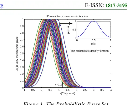
The concept of probabilistic fuzzy sets have been proposed to capture uncertainties with both stochastic and fuzzy features [16] by introducing probability into the traditional fuzzy set described by center and width. Based on considering the random variation from the center of the traditional Gaussian fuzzy set, the random variation was introduced into the membership functions. So in probabilistic fuzzy set, for an input x , there no longer is a single value or values for the membership function; instead, the membership function becomes a random variable that can be described by the secondary PDF as shown in Figure 1.

As such, a 3-dimention membership function including the fuzzy dimension and the probabilistic dimension is hinted in the probabilistic fuzzy set, which makes it able to handle the information with both fuzzy and stochastic uncertainties existing in the process.

-1 -0.5 0 0.5 1 1.5 2 2.5 3 3.5 4

0 0.1 0.2 0.3 0.4 0.5 0.6 0.7 0.8 0.9 1

x(Crisp input)

u

(x

)(

F

u

z

y

m

e

m

b

e

rs

h

ip

g

ra

d

e

Primary fuzzy membership function

0 0.5 1

u(x) pr

(x

,u

)

x=1.2

[image:2.612.318.521.73.240.2]

The probabilistic density function

Figure 1: The Probabilistic Fuzzy Set

2.2 Probabilistic Fuzzy Logic System

Similar to the ordinary fuzzy logic system, the PFLS still has operations of fuzzification, inference engine and defuzzification. Different to the ordinary fuzzy logic system, the PFLS uses the probabilistic fuzzy set that is described by a three-dimensional MF.

The systematic design procedure which is given to design the probabilistic fuzzy logic system for process modeling is as follows:

Step 1) The fuzzy c -mean variance (FCMV) algorithm is used to obtain the clustering results as shown in Figure 2. The ellipses denote the clustering, the c is the fine clustering center, where _i

n is the number of cluster partition.

Step 2) Cluster centers are projected to x and 1 2

x axis to obtain the Gaussian membership function of each clustering. With the clustering result, the secondary PDF can be determined by considering the variation from the mean of Gaussian function.

Step 3) The inference in PFLS is based on the fuzzy rules as follows:

1, ,

1

,

: ...

... ,

j _i i j

n j n

Rule j If x is A and and x is A

and and x is A

j

Then y is B (1)

where Ai j, (i=1, 2,..., ) (n j=1, 2,..., )j and B are j

probabilistic fuzzy sets.

x2

u

k x

1

c

2

c

(

)

u

x

(

))

p

u

x

(3)

877 Step 4) The defuzzification operation in the PFLS is concerned with the probabilistic fuzzy set instead of ordinary fuzzy sets. A probabilistic defuzzification method is used for the PFLS, where mathematical expectation of the centroid output is computed as the final crisp output. The probabilistic defuzzification improves the traditional defuzzification method with the probabilistic processing method.

The previous probabilistic fuzzy set is constructed through randomizing the center of the Gaussian type fuzzy set, the choice of the primary membership functions units of fuzzy remains the important problems for such systems. So it may be interesting to study the bell-shaped primary MF whose shape will be changing with different parameter.

3. CONSTRUCTION OF BELL-SHAPED

PROBABILISTIC FUZZY SET

In this section, based on bell-shaped membership function, a new type of probabilistic fuzzy set will be proposed.

3.1 The Bell-shaped Membership Function The primary MF as bell type is described in (2) shown in Figure 3.

2

1

b

U

x c ξ

=

 ₋ 

+ 

 

(2)

Obviously, a bell-shaped membership function is characterized by three parameters: center c, width

ξ , and slopes b. When b=2, the bell-shaped membership function degenerates into a π membership function which approximates a Gaussian function. We see that by adjusting the slope b, a bell-shaped membership function can approximate Gaussian functions and π functions. With bell-shaped membership function modeling, the Gaussian and π MF consists just in the parameter values.

-1 -0.5 0 0.5 1 1.5 2 2.5 3 3.5 4

0 0.1 0.2 0.3 0.4 0.5 0.6 0.7 0.8 0.9 1

x(Crisp input)

u

(x

)(

F

u

z

y

m

e

m

b

e

rs

h

ip

g

ra

d

e

b=2

[image:3.612.336.514.79.221.2]

b=6

Figure 3. Bell-Shaped Fuzzy MF With Different Parameter B

3.2 The Construction of Bell-based Probabilistic Fuzzy Set

3.1.1 The bell-shaped probabilistic fuzzy set with randomizing center

Based on the central limit theory, the distribution of the center c in equation (2) can be seen as a random variable following the normal distribution described as

2

~ ( , )

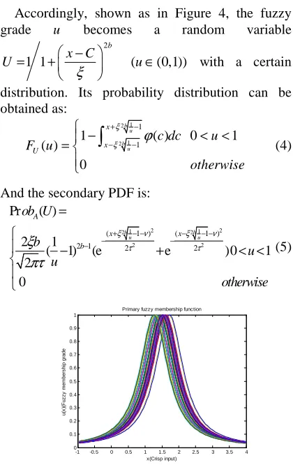
C Nν τ (3) Accordingly, shown as in Figure 4, the fuzzy grade u becomes a random variable

2

1 1 ( (0,1))

b

x C

U u

ξ

 ₋ 

= +  ∈

  with a certain

distribution. Its probability distribution can be obtained as:

1 2

1

1 ( ) 0 1

( ) 0

b u b

u x x U

c dc u F u

otherwise

ξ

ξ ϕ

+ −

− −



− < <



=



∫

₍₄₎

And the secondary PDF is:

2 2

1 1

2 2

( 1 ) ( 1 )

2 1 2 2

Pr ( )

2 1

( 1) (e e )0 1

2 0

b b

u u

A

x x

b

ob U b

u u

otherwise

ξ ν ξ ν

τ τ

ξ πτ

+ − − − − −

− −

−

=



 ₋ ₊ _{< <}

  

(5)

-1 -0.5 0 0.5 1 1.5 2 2.5 3 3.5 4

0 0.1 0.2 0.3 0.4 0.5 0.6 0.7 0.8 0.9 1

x(Crisp input)

u

(x

)(

F

u

z

y

m

e

m

b

e

rs

h

ip

g

ra

d

e

[image:3.612.313.523.371.704.2]

(4)

878

Proof：：：：

Suppose center C is a random variable following normal distribution described as:

2

~ ( , )

C Nν τ (6)

Then the density function is

2 1 ( )( ) 2 1 ( ) 2 C

C e ντ

πτ

− −

Φ = (7)

The random variable fuzzy grade is

2

1 1 ( (0,1))

b x c U u ξ  ₋  = +  ∈

  . Since U is

non-monotonic, it is monotonically decreasing in (0,+∞), so the distribution function of U can be obtained as following:

Obviously, when u≤0, the distribution function is

( ) ( ) 0

U

F u =P U <u = (8)

When 0< <u 1

1 1 2 2 2 1 1 2 2 1 1 2 2 1 1 ( ) 1 ( ) ( ) 1

( 1) ( 1)

( 1) 1 ( 1)

( ) 1 ( )

b b u u U b b b u u b b u u x x F u

P U u P u

x c

P x or P x c

P c x P c x

c dc c dc

ξ ξ

ξ

ξ ξ ξ

ξ ξ

ϕ ϕ

− − + −

−∞ −∞

= < = <

 ₋ 

+ 

 

= − > − − < − −

= < − − + − < + −

=

_∫

+ −

_∫

(9)

In terms of integral additive, (9) can be written as:

1 1 1

2 2 2

1 2 1 2 1 2

1 1 1

1

( ) 1 [ ( ) ( ) ]

1 ( )

b b b

u u u

b u b u b u

x x x

x x

x

c dc c dc c dc

c dc

ξ ξ ξ

ξ

ξ ξ

ϕ ϕ ϕ

ϕ − − − − + − −∞ −∞ − − + − − − + − + = −

∫

(10)

Thus, the probabilistic distribution of U is

equation (4).

Again, we consider the first derivative of u , the density function can be obtained from Variable Limit Integral Derivation Formula as:

2 1 2 2 2 1 2 2 2 2 1 1 2 2 2 2

( 1 )

1

2 2

( 1 )

1

2 2

2 1

( 1 ) ( 1 )

2 2

1

( ) [ e ( 1)

2

1

e ( 1) ]

2

2 1

( 1)

2

(e e )

b u b u b b u u x b U u x b u b x x

F u x

x b u ξ ν τ ξ ν τ

ξ ν ξ ν

τ τ ξ πτ ξ πτ ξ πτ + − − − − − − − − + − − − − − − − ′ = − + − ′ ′ − − − = − + (11)

It follows that the secondary PDF is equation (5).

3.1.2 The bell-shaped probabilistic fuzzy set with randomizing width.

In engineering applications, based on the random sampling principle, in the process of repeatedly extracting samples that follows the normal distribution, if the samples number n is large enough [17], the distribution of variance θ of these samples will gradually approach to the normal distribution, which can be described as:

2

( , )

N

θ α β (12)

where θ is the variance, α denotes the mean of θ and β denotes the variance of θ.

In equation (2), the width ξ is regarded as the variance θ of equation (12), it can be seen as a random variable following the normal distribution described as

2

~N m( , )

ξ σ (13)

Accordingly, shown as in Figure 5, the fuzzy grade u becomes a random variable

2 1 1 b x c U

ξ

 ₋  = + 

  with a certain distribution. Its probability distribution can be obtained as:

2 2 1 1 1 1

( ) 0 1

( ) 0 b b x c u x c U u d u F u otherwise

ϕ ξ ξ

− − − − −   < <  =   

∫

₍₁₄₎

And the secondary PDF is:

2 2 2 2 2 2 ( ) ( ) 1 1 1 1 2 2 2

Pr ( ) ₍ ₎₀ ₁

2 0

b b

x c x c

m m

u u

A

x c

ob u _e _e _u

bu otherwise σ σ − − − − − − − − −    ₋

= ₊ _{< <}

  

(15)

(5)

879

-1 -0.5 0 0.5 1 1.5 2 2.5

0 0.1 0.2 0.3 0.4 0.5 0.6 0.7 0.8 0.9 1

x(Crisp input)

u

(x

)(

F

u

z

y

m

e

m

b

e

rs

h

ip

g

ra

d

e

Figure 5. Fuzzy MF In Bell-Shaped Probabilistic Fuzzy Set For The Perturbed Width

4. MODELING ANALYSIS OF

BELL-SHAPED PROBABILISTIC FUZZY SETS In this section, based on the proposed PFS, bell-shaped MF with randomizing center (Bell_center PFS) and bell-shaped MF with randomizing width (Bell_width PFS), the related PFLSs are constructed to a modeling problem to demonstrate some properties, and to investigate their distinctive modeling capability in stochastic circumstance.

4.1 Modeling Process

4 2

0.9( )

1.4( ) ( ) 0.5

x y

x x

ξ

ξ ξ

+ =

+ + + +

(16)

where y is the output, x is the input with random perturbation ς.

In engineering progress, there is multiform random disturb, for example: Gaussian noise, random perturbation with uniform distribution and so on. To obtain input with different random disturb, the following ten kinds of random perturbation ς are considered:

(1) Random perturbation with Binomial distribution, parameters (5, 0.1), (10, 0.3), and (15, 0.5) are considered.

(2) Random perturbation with F distribution, parameters (1, 2), (2, 5), and (5, 11) are considered.

(3) Random perturbation with Gamma distribution, parameters (1, 2), (2, 2), and (5, 1) are considered.

(4) Random perturbation with normal distribution, parameters (0, 1), (-2, 0.5), and (0, 0.2) are considered.

(5) Random perturbation with geometric distribution, parameters 0.2, 0.5, and 0.8 is considered.

(6) Random perturbation with uniform distribution, parameters (0, 1), (0, 0.5), and (0, 1.5) are considered.

(7) Random perturbation with chi-square distribution, parameters 1, 3, and 5 are considered.

(8) Random perturbation with Poisson distribution, parameters 1, 4, and 10 are considered. (9) Random perturbation with T distribution, parameters 1, 5, and 10 are considered.

(10) Random perturbation with exponential distribution, parameters 0.5, 1, and 1.5 are considered.

And the strength coefficient is k=0.05. Three kinds of parameters for each random perturbation are considered.

For each input with different random perturbation, Bell_center -based PFLS and Bell_width -based PFLS are constructed to model the nonlinear system (13) as following:

Step 1) Collect input–output data n=100. Step 2) Obtain the clustering results parameters (clustering center c , width ξ ) by the fuzzy c -mean variance (FCMV) algorithm. The number of

clustering center c%=5 and b=2 and b=4.

Step 3) The bell-shaped membership function of the antecedent part is obtained to construct fuzzy

if −then rules. Then parameters (the mean ν and

m , the variance τ and σ ) for second PDF which are expressed in equation (5) and equation (15) can be determined by randomizing the center and the width. The l−th rule in PFLS is:

: l, l

Rule l if x is A then y is B (17)

Step 4) The simulation comparison of Bell_center

-based PFLS, Bell_width-based PFLS and Gau_center -based PFLS is carried out. RMSE is used here as:

2

1

( ( ) ( ))

n

e k

RMSE y k y k

n =

=

∑

− (18)

where n=100 is the number of testing data, y k( )

is the desired output and y ke( ) is the estimated output.

4.2 Results

For each random perturbation, the comparison of approximation error |y−ye| between Bellcenter

(6)

880

0 10 20 30 40 50 60 70 80 90 100

0 0.02 0.04 0.06

Binomial-Error (5,0.1)

0 10 20 30 40 50 60 70 80 90 100

0 0.02 0.04 0.06 0.08

Binomial-Error (10,0.3)

0 10 20 30 40 50 60 70 80 90 100

0 0.02 0.04 0.06

Binomial (15,0.5)

0 10 20 30 40 50 60 70 80 90 100

0 0.05 0.1

Geometric-Error (0.2)

0 10 20 30 40 50 60 70 80 90 100

0 0.02 0.04 0.06 0.08 0.1

0 10 20 30 40 50 60 70 80 90 100

0 0.01 0.02 0.03 0.04 0.05

0 10 20 30 40 50 60 70 80 90 100

0 0.05 0.1 0.15 0.2

T-Error (1)

0 10 20 30 40 50 60 70 80 90 100

0 0.02 0.04 0.06 0.08 0.1

T-Error (5)

0 10 20 30 40 50 60 70 80 90 100

0 0.02 0.04 0.06 0.08

T-Error (10)

0 10 20 30 40 50 60 70 80 90 100

0 0.02 0.04 0.06 0.08 0.1

Gamma-Error (1,2.0)

0 10 20 30 40 50 60 70 80 90 100

0 0.02 0.04 0.06 0.08 0.1

Gamma-Error (2,2.0)

0 10 20 30 40 50 60 70 80 90 100

0 0.05 0.1

Gamma-Error (5,1.0)

0 10 20 30 40 50 60 70 80 90 100

0 0.02 0.04 0.06

Normal-Error (0,1)

0 10 20 30 40 50 60 70 80 90 100

0 0.01 0.02 0.03 0.04

Normal-Error (-2,0.5)

0 10 20 30 40 50 60 70 80 90 100

0 0.01 0.02 0.03

(7)

881

0 10 20 30 40 50 60 70 80 90 100

0.02 0.04 0.06 0.08 0.1

Chi-square-Error (1)

0 10 20 30 40 50 60 70 80 90 100

0 0.05 0.1

0 10 20 30 40 50 60 70 80 90 100

0 0.02 0.04 0.06 0.08 0.1

0 10 20 30 40 50 60 70 80 90 100

0 0.02 0.04 0.06 0.08

Poisson-Error (1)

0 10 20 30 40 50 60 70 80 90 100

0 0.05 0.1

Poisson-Error (4)

0 10 20 30 40 50 60 70 80 90 100

0 0.05 0.1

[image:7.612.90.517.72.268.2]

Poisson-Error (10)

Figure 6. The Comparison Of Approximation Error (|y−ye|) With Bellcenter-Based PFLS (Blue Solid), width

Bell -Based PFLS (Red Dash Dot) And Gau_center-Based PFLS (Black Dot) Corresponding To The Input With Different Random Disturb.

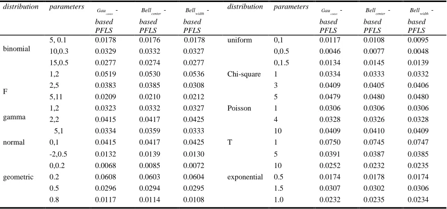
Table 1:: The Results Of Approximation Error (|y−ye|) With Bellcenter-Based PFLS, Bellwidth-Based PFLS And

center

Gau -Based PFLS Corresponding To The Input With Different Random Disturb.

distribution parameters

center

Gau -based PFLS

center

Bell -based PFLS

width

distribution parameters

center

Gau -based PFLS

center

width

binomial

5, 0.1 0.0178 0.0176 0.0178 uniform 0,1 0.0117 0.0108 0.0095

10,0.3 0.0329 0.0332 0.0327 0,0.5 0.0046 0.0077 0.0048

15,0.5 0.0277 0.0274 0.0277 0,1.5 0.0134 0.0145 0.0139

F

1,2 0.0519 0.0530 0.0536 Chi-square 1 0.0334 0.0333 0.0332

2,5 0.0383 0.0385 0.0308 3 0.0409 0.0405 0.0406

5,11 0.0209 0.0210 0.0212 5 0.0479 0.0480 0.0480

gamma

1,2 0.0323 0.0332 0.0327 Poisson 1 0.0306 0.0306 0.0306

2,2 0.0415 0.0417 0.0425 4 0.0328 0.0326 0.0328

5,1 0.0334 0.0359 0.0333 10 0.0409 0.0410 0.0409

normal 0,1 0.0415 0.0417 0.0425 T 1 0.0750 0.0745 0.0747

-2,0.5 0.0132 0.0139 0.0130 5 0.0391 0.0387 0.0385

0,0.2 0.0068 0.0085 0.0072 10 0.0252 0.0232 0.0235

geometric 0.2 0.0608 0.0603 0.0604 exponential 0.5 0.0174 0.0178 0.0174

0.5 0.0296 0.0294 0.0295 1.5 0.0307 0.0302 0.0306

0.8 0.0117 0.0114 0.0108 1.0 0.0232 0.0235 0.0234

A comprehensive and detailed study to modeling capability of PFS is presented above. From the performance comparison, it is clearly that the modeling performance of Bell_center-based

PFLS and Bell_width-based PFLS is better than that

of Gau_center -based PFLS when input is disturbed by random perturbation with Binomial distribution, geometric distribution, or T distribution. On the other hand, the modeling performance of the three PFLSs turns out the same when input is disturbed by random perturbation with chi-square distribution or Poisson distribution. The reason is that the Bell_center-based

PFLS and Bell_width -based PFLS whose primary

MF will be changing with different parameter have the better potential ability to handle uncertainties than Gau_center-based PFLS under certain stochastic circumstance.

5. CONCLUSION

[image:7.612.87.528.343.549.2]

(8)

882 In the future, more designation may be conducted for PFS, such as PFS with asymmetrical primary MF or secondary PDF. It is believed that the PFS will be very promising for many engineering application.

REFERENCES:

[1]. A.H. Meghdadi and M.-R. Akbarzadeh-T, “Probabilistic fuzzy logic and probabilistic fuzzy systems”, Proceedings of International

Conference on Fuzzy Application in Engineering, IEEE Conference Publishing

Services, January 25-28, 2001, pp. 1127– 1130.

[2]. J. C. Pidre, C. J. Carrillo, and A. E. F. Lorenzo, “Probabilistic model for mechanical power fluctuations in asynchronous wind parks,” IEEE Trans. Power Syst., Vol. 18, No. 2, 2003, pp. 761–768.

[3]. L. A. Zadeh, “Fuzzy sets”, Inform.and

control, Vol. 8, NO.5, 1965, pp. 338–353.

[4]. L. A. Zadeh, “The concept of a linguistic variable and its application to approximate reasoning—I”, Inform. Sci., Vol. 8, No.4, 1975, pp. 199–249.

[5]. Nilesh N. Karnik, Jerry M. Mendel and Qilian Liang, “Type-2 fuzzy logic systems”,

IEEE Transations on Fuzzy Systems, Vol. 8,

No. 6, 2006, pp. 808-821.

[6]. Mendel, J.M, “An introduction to type-2 fuzzy logic systems,” Univ. Southern

California, Rep., 1998,

http://sipi.usc.edu/˜mendel/report.

[7]. L. A. Zadeh, “Discussion: Probability theory and fuzzy logic are complimentary rather than competitive,” Technomet., Vol. 37, No. 3, 1995, pp. 271–276.

[8]. M. Laviolette and J. W. Seaman Jr, “Unity and diversity of fuzziness from a probability viewpoint,” IEEE Trans. Fuzzy Syst., Vol. 2, No. 1, 1994, pp. 38–42.

[9]. L.A.Zadeh, “Probability measures of Fuzzy events”, Mathematical Analysis and Applications, Vol. 23, No.2, 1968, pp.

141-150.

[10].Ke-ang Fu, Li-xin Zhang, “Strong limit theorems for random sets and fuzzy random sets with slowly varying weights”,

Information Sciences 178, 2008, pp.

2648-2660.

[11].Puri, M.L., Ralescu, D.A, “Fuzzy random variables”, Journal of Mathematical Analysis

and Applications, Vol. 2, No. 114, 1986, pp.

409-422.

[12].González-Rodríguez, G., Colubi, A., Trutschnig, W, “Simulation of fuzzy random variables”, Information Sciences, Vol. 5, No. 179, 2009, pp. 642-653.

[13].Jonathan M. Garibaldi, Marcin Jaroszewski, and Salang Musikasuwan, “Nonstationary fuzzy sets”, IEEE Transactions on Fuzzy

Systems, Vol.16, No.4, 2008, pp. 122-130.

[14].Jan van den Berg, Uzay Laymak, Willem-Max van den Bergh, “Financial Markets Analysis by Using a Probabilistic Fuzzy Modeling Approach” International Journal

of Approximate Reasoning, Vol.35, No. 3,

2004, pp 291-305.

[15].Z. Liu, H.X. Li, ‘A probabilistic fuzzy logic system for modeling and control’, IEEE

Trans Fuzzy Systems, Vol. 13, No. 6, 2005,

pp. 848-859.

[16].Han-Xiong Li and Zhi Liu, “A Probabilistic Neural-Fuzzy Learning System for Stochastic Modeling”, IEEE Trans. Fuzzy Syst., Vol. 16, No. 4, 2008, pp. 384–390.

[17].Minhaz Fahim Zibran, “CHI-Squared Test of