Geometric Structure Extraction and Reconstruction

(1)

Geometric Structure Extraction and Reconstruction

Inauguraldissertation

der Philosophisch-naturwissenschaftlichen Fakultät der Universität Bern

vorgelegt von

Shihao Wu

von China

Leiter der Arbeit: Prof. Dr. M. Zwicker

Universität Bern Prof. Dr. M. Wand Universität Mainz

(2)

(3)

Geometric Structure Extraction and Reconstruction

Inauguraldissertation

der Philosophisch-naturwissenschaftlichen Fakultät der Universität Bern

vorgelegt von Shihao Wu

von China

Leiter der Arbeit: Prof. Dr. M. Zwicker

Universität Bern Prof. Dr. M. Wand Universität Mainz

Von der Philosophisch-naturwissenschaftlichen Fakultät angenommen.

Bern, 6.7.2018 Der Dekan:

(4)

(5)

i

Abstract

Geometric structure extraction and reconstruction is a long-standing problem in research communities including computer graphics, com-puter vision, and machine learning. Within different communities, it can be interpreted as different subproblems such as skeleton ex-traction from the point cloud, surface reconstruction from multi-view images, or manifold learning from high dimensional data. All these subproblems are building blocks of many modern applications, such as scene reconstruction for AR/VR, object recognition for robotic vision and structural analysis for big data. Despite its importance, the extrac-tion and reconstrucextrac-tion of a geometric structure from real-world data are ill-posed, where the main challenges lie in the incompleteness, noise, and inconsistency of the raw input data. To address these chal-lenges, three studies are conducted in this thesis: i) a new point set representation for shape completion, ii) a structure-aware data con-solidation method, and iii) a data-driven deep learning technique for multi-view consistency. In addition to theoretical contributions, the algorithms we proposed significantly improve the performance of sev-eral state-of-the-art geometric structure extraction and reconstruction approaches, validated by extensive experimental results.

Keywords. Points representation, meso-skeleton, consolidation,

da-ta consolidation, filtering, clustering, dimensionality reduction, mani-fold denoising, generative adversarial network, multi-view reconstruc-tion, multi-view coherence, specular-to-diffuse, image translation

(6)

(7)

iii

Acknowledgements

First and foremost I want to thank my advisor Prof. Matthias Zwick-er. It has been a great honor and pleasure working with him. I’m thankful for all his contribution of time, care, effort, ideas, joy, moti-vation, teaching, and funding that give me the best Ph.D. experience one could ask for. None of my research work could have been pos-sible without his intellectual guidance and mental support. He is such an excellent role model of life-work balance, creative, curiosity, optimistic, generous, and kindness that teaches me how to become a happier, healthier, and more conscious person, which makes this journal truly invaluable.

I’m also grateful for working in Bern with those incredible CGG members. Dragana Esser gave me the warmest welcoming and help me settle down in Bern thoughtfully. She keeps our lab well organized and makes everything easy going. She is always there and walks me through many life troubles. Marco Manzi is friendly, productive, and full of interesting ideas. It’s always pleasant being with and learning something from him, e.g. the time we spent together in Siggraph Asia still fresh to me. Daniel Donatsch is cheerful, dependable, and sport-ing, kind-hearted. He always offers his help before I ask. He is also my coach for indoor cycling and certainly convince me the benefits of doing sport. Peter Bertholet is so talented, humble, and being patient as my teacher of mathematics and geometry. He contributes to the elegant formulation for our theoretical analysis in the SAF work. We had a wonderful time attending conferences, hiking, and board gam-ing. Tiziano Portenier is quiet, efficient and cooperative. He teaches me a lot, especially the deep learning techniques. He wrote a pro-fessional technical description of S2Dnet shortly before the deadline. Daljit Singh is a close friend and his passion for life and research is contagious. Siavash A. Bigdeli has many good qualities I’m learning from, e.g., confidence, curiosity, and heartiness.

I would also like to offer my sincere thanks to my mentors over the years. Prof. Hui Huang is a co-supervisor of both my master and Ph.D. degree. She is amiable, determined, aspiring, being the backbone of

(8)

iv

our projects, and keep encouraging and cultivating me to be a good researcher. Prof. Guiqing Li is my master supervisor who opened the door for me doing research. He is tireless, unselfish and popular to the students. We keep collaborating and published two works during my Ph.D. study. Prof. Daniel Cohen-Or is the top of the top researcher in the field, who inspires most of the ideas of my research work and keep lightening and driving the project to success with his dedication. He invited me to visit his lab in the table-via university and his hearty families, which is an unforgettable experience. Prof. Minglun Gong is brilliant, caring and skillful. The soul of my research works would have been incomplete without his great contributions.

I would like to take this opportunity to thank all the collaborators in my research works, including: Matan Sela, Xuequan Lu, Honghua Chen, Yinglong Zheng, Jie Mei, Liqiang Zhang, Wei Sun, Pinxin Long, Jiacheng Ren, Jinfeng Ou, Xiaohui Zhou, Simone Raimondi, Prof. Ron Kimmel, Prof. Oliver Deussen, Prof. Baoquan Chen, Prof. Uri Ascher, Prof. Hao Zhang, and etc..

We are also lucky of meeting great friends in these four years who gave us lots of help and joy: Niclas Scheuing, John Sivell, Vittorio Caggiano, Sukhbeer Kaur Sabharwal, Laura Höylä, Anita Sobe, Céline Dizerens, Rava Pourboghrat, Peppo Brambilla, Gian Calgeer, Stefan Moser, Fabrice Rousselle, Givi Meishvili, Simon Jenni, Adrian Wälchli, Qiyang Hu, Meiguang Jin, Zan Li, and etc.

The lists of people who helped me in the journey have no ends. In particular, I can’t thanks enough to Prof. Michael Wand for being the co-referee of my thesis and Prof. Paolo Favaro being the head of defense community. Their generous support during my thesis writing period makes this work finish in time.

Last but not least, I thank my parents Qinghua Wu and Huaying Luo for their unconditional love. They offer me absolute freedom and support to pursue my goals. My heartiest gratitude goes to my beloved wife Xiaowei (Magenta) Zeng. Her smile and bravery make us overcome every day’s challenges effortlessly. Her kindness and friendliness bring us the happiness and friends. Her artistic taste deeply flows into my works. Her love makes every impossible possible.

(9)

v I thank everyone for everything and devote this thesis.

(10)

(11)

List of Figures

1.1 Examples of geometric structure in the natural . . . 10

1.2 A piece of ancient red ochre . . . 11

1.3 Some modern data acquisition techniques . . . 11

1.4 Applications of geometric structure extraction and re-construction . . . 12

1.5 Main challenges of geometric structure extraction and reconstruction . . . 15

2.1 Insensitivity of theL1-median (red dot) to noise and outliers in the data. . . 21

2.2 LocalizedL1-Median using different size of local neigh-borhood size . . . 22

2.3 With and without repulsion term. . . 22

2.4 LOP using different size of local neighborhood size . . 23

2.5 Illustration of a neuron activation with three input sig-nals. . . 24

2.6 An example of a neural network structure. . . 26

2.7 A visualization of backpropagation. . . 27

2.8 A convolutional layer. . . 29

2.9 An example of convolutional neural network. . . 30

2.10 An example of deconvolutional layer. . . 32

2.11 The structure of an autoencoder. . . 33

2.12 An overview of GAN. . . 34

(14)

4 LIST OF FIGURES 3.1 Illustration of deep points representation. . . 38

3.2 Comparison of the reconstruction of the input, output of WLOP, and output of our consolidation. . . 40

3.3 Overview of Deep points consolidation . . . 42

3.4 Generating anchor points by sinking consolidated points 46

3.5 Generation of meso-skeleton . . . 47

3.6 The anisotropic neighborhoods defined along local PCA axes . . . 51

3.7 Consolidation of surface points based on the formed meso-skeleton . . . 52

3.8 Surface completion of large missing areas . . . 53

3.9 The impact of the parameterω . . . 62

3.10 Another example of the impact of the parameterω . . 63

3.11 The impact of the neighborhood size parameterσp . . 64 3.12 Reconstructions for a synthetic model under different

neighborhood size parametersσp . . . 65 3.13 A comparison among the Poisson surface reconstructions 66

3.14 Results on standard benchmark 3D scans . . . 66

3.15 Handling objects with complicate thin and non-tubular structures . . . 67

3.16 Consolidation for an incomplete scan . . . 68

3.17 Quantitative evaluation on reconstruction accuracy . . 69

3.18 Quantitative evaluation on reconstruction accuracy us-ing a synthetic toy model . . . 70

3.19 Quantitative evaluation on reconstruction accuracy for noise corrupted scans of the toy model . . . 71

3.20 Quantitative evaluation on reconstruction accuracy us-ing a synthetic gundam model . . . 72

3.21 Quantitative evaluation on reconstruction accuracy for noise corrupted scans of the gundam model . . . 73

3.22 Post-processing for reconstructing fine geometry details and sharp features . . . 74

3.23 Dpoints consolidation for thin structures and close-by surface sheets . . . 75

(15)

LIST OF FIGURES 5 3.25 Dpoints representations under different shape priors . 75

3.26 Stress test performed by corrupting the scan data of a real complex object . . . 76

4.1 A challenging example with two intertwined clusters, corrupted with noise . . . 78

4.2 Consolidation process using anisotropic SAF . . . 87

4.3 Clustering without (SAF) and with anisotropic repul-sion (A-SAF) . . . 88

4.4 We illustrate the iterative consolidation process in a 2D example . . . 90

4.5 Empirical estimate and theoretical prediction . . . 90

4.6 Convergence in different dimensions and with median repulsion . . . 91

4.7 We compare mean and median repulsion . . . 92

4.8 Our theory can predict the convergence for high dimen-sional data . . . 93

4.9 Dimensionality reduction and clustering . . . 94

4.10 Performance of dimensionality reduction . . . 97

4.11 Improved performance of different clustering techniques 98

4.12 Dimensionality reduction and clustering . . . 100

4.13 Additional clustering examples of low dimensional struc-tures corrupted with high dimensional noise . . . 101

4.14 We illustrate how spectral clustering benefit from our data consolidation technique . . . 102

4.15 SAF performance with increasing dimensionality of the data . . . 104

4.16 Scores of SAF with increasing dimensionality . . . 105

4.17 The performance of our consolidation with data density increasing . . . 105

4.18 Comparison of different noise levels using 2D moons . 108

4.19 Comparison of different noise levels using 2D concen-tric circles . . . 110

(16)

6 LIST OF FIGURES 4.21 Performance under different noise levels and for

differ-ent datasets . . . 113

4.22 Clustering the real MINST data with different 3D em-bedding spaces . . . 115

4.23 The scores of clustering the MINST data with different 3D embedding spaces . . . 116

4.24 The scores of clustering the Yale face data . . . 116

4.25 The performance of our consolidation with increasing number of target clusters in the Yale face data . . . 118

4.26 A parameter selection strategy guided by our conver-gence criterion . . . 120

4.27 Further discussion of parameter selection . . . 121

5.1 Specular-to-diffuse translation of multi-view images . . 124

5.2 Overview of S2Dnet . . . 128

5.3 Gallery of our synthetically rendered specular-to-diffuse training data . . . 128

5.4 Two examples of the SIFT correspondences pre-computed for our training . . . 131

5.5 Illustration of the generator and discriminator network 134

5.6 Qualitative translation results on a synthetic input se-quence consisting of 8 views . . . 137

5.7 Qualitative surface reconstruction results on 10 differ-ent scenes . . . 139

5.8 Gallery of our glossy-to-diffuse real-world training data 140

5.9 Qualitative translation results on a real-world input se-quence consisting of 11 views . . . 141

5.10 Qualitative surface reconstruction results on 7 different real-world scenes . . . 142

5.11 A sample of our real-world dataset . . . 144

5.12 Gallery of our glossy-to-diffuse results of 40 synthetic and 10 real-world scenes . . . 145

5.13 Qualitative comparison of image translation and sur-face reconstruction on a synthetic sequence consisting of 10 views . . . 146

(17)

LIST OF FIGURES 7 5.14 Another set of image translation and surface

reconstruc-tion comparison on a synthetic input sequence consist-ing of 10 views . . . 147

(18)

(19)

Chapter 1

Introduction

Geometry existed before the creation.

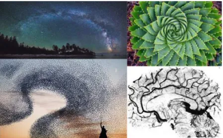
Plato Geometric structure is beautiful and everywhere, see Figure1.1

for a few examples in our nature. As one of the earliest forms of human art, our ancestors engraved geometric pattern on stones, see Figure1.2, around 100,000 years ago. Our modern data acquisition techniques such as CT scanner, light field camera, and 3D laser scan-ner, as shown in Figure1.3, allow us capturing massive real-world geometric data in a few seconds. However, given these raw input data, the extraction and reconstruction of the geometric structure remains a long-standing problem shared by research communities including computer graphics, computer vision, and machine learn-ing. Researchers in different fields may hold a different view for this problem depending on what types of input data they are work-ing with. For example, it can be viewed as a problem of skeleton extraction from the point cloud [130], surface reconstruction from multi-view images [118], and manifold learning from high dimen-sional data [19]. All these subproblems have gained much attention in recent years, driven by a wide range of modern applications, such

(20)

10 CHAPTER 1. INTRODUCTION as scene reconstruction for AR/VR, object understanding for robotic vision, and structural analysis for big data, as shown in Figure1.4. It is also tightly related to those big questions in artificial intelligence: how would a machine be truly aware of the geometric structure with their own sensing? Can it extract, reconstruct and understand the underlying structure of the information consciously, creatively, and deeply? What governs the structure of all? Our exploration of such a fundamental problem is an exciting and everlasting journey.

Figure 1.1: Examples of geometric structure in the natural. From top left to bottom right: a nice curve of our milki-way, a plant with spiral structure, an omega shape formed by birds, and the tree structure of our brain. Credit: WALLPAPERIA, Alanna, Alain, Pinterest.

(21)

1.1. PROBLEM STATEMENT 11

Figure 1.2: A piece of red ochre with a deliberate zigzag engraving from Blombos cave, South Africa. Credit: Anna Zieminski/AFP/Getty and Chris Henshilwood.

Figure 1.3: Some modern data acquisition techniques. From left to right are: medical scanner, light field camera, 3D scanner. Credit: RAYMOND R. HOULE CONSTRUCTION, LYTRO, and [155].

1.1

Problem Statement

Let us first define the scope of the problem addressed in this thesis. We assume the raw input data to our problem are commonly used media like 2D images, 3D point cloud, or high dimensional scientific data. The output geometric structure we seek for is a continuous, intrinsic, and meaningful representation of the input data. The struc-ture representation can be in the form of a skeleton, surface, manifold, etc. Ideally, the underlying geometric structure of the data can be best extracted and reconstructed when the input data is intact, clean and consistent. However, the reality is quite the opposite. All kinds of

(22)

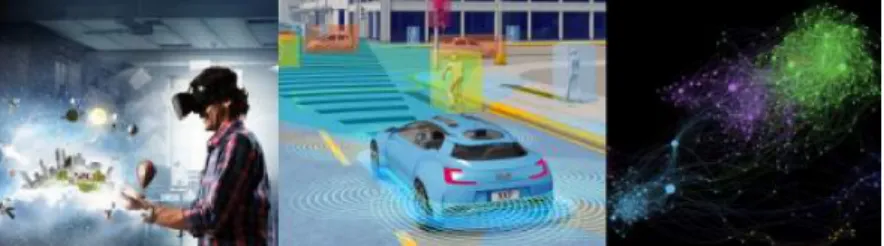
prac-12 CHAPTER 1. INTRODUCTION

Figure 1.4: Applications of geometric structure extraction and recon-struction: AR/VR, autonomous car, data visualization and analysis. Credit: Sergey Nivens, OVERSQUARE AUTOMOTIVE, Kimo Quain-tance.

tical and physical limitations make the input data incomplete, noisy, and inconsistent. Hence our research problem of geometric structure extraction and reconstruction from the imperfect raw input data is ill-posed. Knowing that a perfect solution to such ill-conditioned prob-lem does not exist, we can discuss in the following how we approach these three challenges, i.e., the incomplete, noisy, and inconsistent nature of the data.

Incompleteness. Almost everything in our universe, including a

molecule, a stone, a tree, a forest and even a distribution of some high dimensional data, has its unique structure and contains a large amount of geometric information. Capturing and storing all these information is an ambitious yet unpractical goal, despite the fast de-velopment of advanced data acquisition techniques [155]. Besides, one common limitation of all data collection approaches is that the cost of the data acquisition goes up quickly as the increase of data completeness. For example, while it cost almost nothing to take a 2D selfie image, fully scanning a 3D surface or volume of the human body can be expensive and time-consuming. A sacrifice of completeness of-ten has to be made for a low price of data. Therefore, it is desirable to complete the missing geometric information for those incomplete data, based on reasonable prior knowledge [11] such as symmetry,

(23)

1.1. PROBLEM STATEMENT 13 skeleton, smoothness, correspondence, topology, functionality, etc. D-ifferent priors favor dD-ifferent types of input data.

We focus our study of the data completion problem on 3D point clouds, which are acquired from devices like laser scanners and depth cameras that are widespread. A raw point cloud data is a set of data points in space that represents the external surfaces of the object. As shown in Figure1.5(a), the point cloud is often incomplete, as a result of self or inter-object occlusion, inapplicable material, misalignment, unreachable viewpoints, or the acquisition of time-varying data from a single view [142]. Such data imperfection has greatly limited the application of this innovative data representation for many years and remains an open problem in research. As one direction approaching this problem, we proposed a new point set representation method in

Chapter3that allows a joint optimization of the skeleton extraction

and surface completion of an object.

Noise and outliers. Like the data incompleteness, noise and

out-liers are well-known data imperfections that are caused by inevitable limitations of data observation and collection approaches, as shown in Figure1.5(b). Given such noisy and outlier-ridden input data, sci-entists in statics, signal processing, and machine learning have spent tremendous time and effort in designing robust denoising algorithms that reveal and preserve the intrinsic structure of the data. The key to a successful algorithm is an insightful observation of the input data. Therefore, different denoising algorithms have been developed for different types of media such as audio, images, and point clouds. We focus our study on one kind of denoising method that works particu-larly well for point-based data representation. This method, named Locally Optimal Projection (LOP), is proposed by Lipman et al. [85] in 2007 for point cloud denoising. The core insight of LOP is a regulariza-tion term for uniform points distriburegulariza-tion that maintains the structure of data while denoising. We introduce the basic of LOP inChapter2.

InChapter4, we made an important theoretical analysis of LOP about

the convergence criterion, revealing its relation to classical algorithms like mean shift and manifold denoising, and demonstrating its power

(24)

14 CHAPTER 1. INTRODUCTION in applications like clustering and dimensionality reduction.

Inconsistency. Caused also by the limitations of existing data

ac-quisition techniques, our input data is usually captured by multiple observations of the same target but from different views. Given such multi-view data, the extraction of data correspondence and the re-construction of the target model are difficult, if not impossible. The challenge is twofold. First, the information of the observer, e.g. the camera positions, are unknown or unreliable. Second, irrelevant en-vironmental factors that affect the outcome of the observation form different views, e.g. illumination and material, are also unknown and complex.

While these two issues are common for many types of data, the data inconsistency challenge in our study is specifically referred to the appearance incoherency in 3D reconstruction from multi-view images, as shown in Figure1.5(c). One rather strong assumption shared by many multi-view 3D reconstructions is that the target objects are pre-dominantly diffuse. This assumption suggests that the appearance of the model are mostly consistent across different views, which is impor-tant for the computation of image correspondences through feature matching and the improvement of the reconstruction quality through shape-from-shading [79]. However, when the object is not diffuse, the appearance of the object changes in different views and the shad-ing cue is not usable without additional prior knowledge like global illumination or shape silhouette [42]. Therefore, the multi-view re-construction of glossy surfaces is a challenging problem. We believe a promising way to approach this problem is data-driven machine learning, because of the fact that our human mind can be trained to recognize the geometric structures in the images regardless of the complexity of the scene. Encouraged by the success of deep learning algorithms in image processing, we addressed this problem in Chap-ter5through a generative adversarial network (GAN) for multi-view specular-to-diffuse image translation, where some basic of GAN is covered inChapter2.

(25)

1.2. CONTRIBUTIONS 15

Figure 1.5: Main challenges of geometric structure extraction and reconstruction: incompleteness, noise and outliers, and inconsistency. Credit: [58], [151], and [36].

Goals. Aiming to advance research in dealing with the

aforemen-tioned main challenges, in this thesis, the goal we pursue in this thesis is to explore optimization and learning techniques to extract and re-construct the underlying geometric structure from raw input such as point cloud, multi-view images, and high-dimensional data. Towards this goal, we first propose a new 3D point sets consolidation method that optimizes both the inner and surface structure simultaneously. Next, we extend our consolidation technique to high dimensional data with a theoretical analysis for parameter selection. Finally, we tackle the appearance inconsistency problem of multi-view images by leveraging the recent success of learning based image-to-image trans-lation approaches. Experimental results show that all of our proposed methods outperform the corresponding state-of-the-art methods, es-pecially in terms of dealing with noise, incompleteness, inconsistency, and outliers of the data.

1.2

Contributions

This thesis contributes in the following three problems:

Deep Points Consolidation [154]. We present a consolidation method

(26)

16 CHAPTER 1. INTRODUCTION is to augment each surface point into adeep pointby associating it with an inner point that resides on the meso-skeleton, which consists of a mixture of skeletal curves and sheets. The deep points repre-sentation is a result of a joint optimization applied to both ends of the deep points. The optimization objective is to fairly distribute the end points across the surface and the meso-skeleton, such that the deep point orientations agree with the surface normals. The optimiza-tion converges where the inner points form a coherent meso-skeleton, and the surface points are consolidated with the missing regions com-pleted. The strength of this new representation stems from the fact that it is comprised of both local and non-local geometric informa-tion. We demonstrate the advantages of the deep points consolidation technique by employing it to consolidate and complete noisy point-sampled geometry with large missing parts.

Structure-aware Data Consolidation [153]. We present a

structure-aware technique to consolidate noisy data, which we use as a pre-process for standard clustering and dimensionality reduction. Our technique is related to mean shift, but instead of seeking density modes, it reveals and consolidates continuous high density structures such as curves and surface sheets in the underlying data while ig-noring noise and outliers. We provide a theoretical analysis under a Gaussian noise model, and show that our approach significantly im-proves the performance of many non-linear dimensionality reduction and clustering algorithms in challenging scenarios.

Specular-to-Diffuse Translation for Multi-View Reconstruction.

Most multi-view 3D reconstruction algorithms, especially when shape-from-shading cues are used, assume that object appearance is pre-dominantly diffuse. To alleviate this restriction, we introduce S2Dnet, a generative adversarial network for transferring multiple views of objects with specular reflection into diffuse ones, so that multi-view reconstruction methods can be applied more effectively. Our network extends unsupervised image-to-image translation to multi-view “spec-ular to diffuse" translation. To preserve object appearance across

(27)

1.3. THESIS ORGANIZATION 17 multiple views, we introduce a Multi-View Coherence loss (MVC) that evaluates the similarity and faithfulness of local patches after the view-transformation. Our MVC loss ensures that the similarity of lo-cal correspondences among multi-view images is preserved under the image-to-image translation. As a result, our network yields signifi-cantly better results than several single-view baseline techniques. In addition, we carefully design and generate a large synthetic training data set using physically-based rendering. During testing, our network takes only the raw glossy images as input, without extra information such as segmentation masks or lighting estimation. Results demon-strate that multi-view reconstruction can be significantly improved using the images filtered by our network. We also show promising performance on real world training and testing data.

1.3

Thesis Organization

InChapter2, two technical backgrounds are introduced, one is LOP

for local structure filtering, the other is GAN for global structure learn-ing.

In Chapter 3we introduce the deep point representation of 3D

point sets. We augment each surface point into adeep pointby associ-ating it with an inner point that resides on the meso-skeleton, which consists of a mixture of skeletal curves and sheets.

Chapter 4 present a structure-aware technique to consolidate

noisy data, which we use as a pre-process for standard clustering and dimensionality reduction.

InChapter5we introduce S2Dnet, a generative adversarial

net-work for transferring multiple views of objects with specular reflection into diffuse ones, so that multi-view reconstruction methods can be applied more effectively.

Chapter6concludes our research and results and briefly describes

(28)

(29)

Chapter 2

Technical Background

2.1

Introduction

For a better understanding of the techniques in the later chapter-s, in this chapter, we briefly introduce two important background techniques: i) Locally Optimal Projection (LOP) for consolidation of low-level structure and ii) Generative Adversarial Network (GAN) for learning high-level structure.

LOP is the base ofChapter3andChapter4, which was originally introduced by Lipman et al. [85] and improved by Huang et al. [57]. Please refer to these two works for a more detailed technical descrip-tion of LOP. GAN is a trending learning method that Chapter 5 is based on. It was introduced by Ian Goodfellow et al. [45] in 2014 and has attracted enormous attention in the past few years. For a more in-depth introduction of GAN, the reader is advised for other literature [44,27,54].

(30)

20 CHAPTER 2. TECHNICAL BACKGROUND

2.2

Locally Optimal Projection

The Locally Optimal Projection operator (LOP) was originally de-signed for surface approximation from point-set data. Given a set of original input pointsQ={qj}j∈J ⊂R3that is typically unorganized,

unoriented, unevenly distributed, noisy and outliers-ridden, the out-put of LOP should be a set of clean sampled pointsX={xi}i∈I ⊂R3,

which in general is much smaller, i.e.,|I|<<|J|, and more organized thanQ, representing the underlying surface ofQ. Formulated as an optimization problem, the energy function of LOP is a combination of data term and repulsion term. The data term is a localized version of theL1-median that robustly projects sample points onto the surface defined by the original points. Since the contraction force of data term tends to attract sampled points to the local density extrema, a repul-sion term is introduced as a regularization of the points distribution by penalizing sampled points being too close to each other.

L1-median. TheL1-median is a simple and powerful statistical tool

that can be regarded as the extension of the univariate median to the multivariate setting [150]. Unlike the usual mean average, L1 -medians is known to be robust to noise and outliers, as shown in Figure 2.1. By definition, the total Euclidean distance between the

L1-median locationxand a set of input points is minimized, i.e.,

x=argminX

j∈J

kx−qjk.

LocalizedL1-median as data term. TheL1-median is a global

cen-ter of a set of points. It can be adapted locally to a point by adding a weight functionθ, i.e.,

x=argminX

j∈J

(31)

2.2. LOCALLY OPTIMAL PROJECTION 21

(a) (b)

Figure 2.1: Insensitivity of the L1-median (red dot) to noise and outliers in the data. The bluish shade of the points reflects the relative weight with respect to theL1-median center.

The weight functionθ(r) =e−r2/(h/2)2 is a fast decaying smooth function with support radius hdefining the size of the supporting local neighborhood. The result of localized L1-median depends on

the initial position of x and the neighorhood size h. As shown in Figure2.2, a single localizedL1-median can not represent a complex

shape no matter whathwe use. Therefore, we are seeking for a set of localizedL1-medians that best approximates the target shape as our

data term, i.e.,

arg min X X i∈I X j∈J kxi−qjkθ(kxi−qjk).

Repulsion term. Applying the L1-median alone tends to yield a

sparse distribution, where local centers are likely accumulated into a set of point clusters; see Figure2.3(a). To avoid such clustering and maintain a proper geometry representation, we need to counteract the attraction force by adding a repulsion force on the structure itself. This brings the final objective function of LOP with two terms:

(32)

22 CHAPTER 2. TECHNICAL BACKGROUND

Figure 2.2: LocalizedL1-Median using different size of local neigh-borhood. arg min X X i∈I X j∈J kxi−qjkθ(kxi−qjk)− X i∈I µi X i0_∈_I_\{_i_} θ(kxi−xi0k),

where the{µi}i∈I are balancing constants among X that can be set by the user. See Figure2.3(b) for the effect of using the replusion term.

Figure 2.3: With and without repulsion term.

Pros and cons of LOP. Besides its robustness to noise and outliers,

the main advantage of the LOP operator is that it work directly on raw point clouds without additional information like mesh connectivity and point normal. The repulsion term allows LOP extract multi-scale structures with nice distribution by using different kernel sizes, as

(33)

2.3. GENERATIVE ADVERSARIAL NETWORK 23 demonstrated in Figure2.4. Some disadvantages of LOP include over-smoothing, failing to deal with large missing data and sensitivity to the selection of parameters. We have proposed some methods that improve LOP to better preserve sharp features [59,88,166,167]. In

Chapter3, we address the shape completion problem based on LOP.

In terms of parameter selection, Lipman et al. [85] have proven that if the data setQis sampled from aC2-smooth surfaceS, LOP operator has an O(h2) approximation order to S, provided that the balanc-ing parameters{µi}i∈I are carefully chosen. We further analysis the relation between{µi}i∈I and neighborhood sizehinChapter4.

Figure 2.4: LOP using different local neighborhood sizes.

2.3

Generative Adversarial Network

In this section, we will first walk through some basic concepts of neural networks. Then, we focus on the theoretical and practical background of Generative Adversarial Networks. Last, we introduce some extension of GAN that serve as the baselines ofChapter4.

Neural network. In 1943, Warren McCulloch and Walter Pitts [92]

created a computational model for neural networks based on mathe-matics and algorithms called threshold logic. Nowadays, the neural network has become the most powerful machine learning tool in many complex tasks in areas like natural language processing and computer

(34)

24 CHAPTER 2. TECHNICAL BACKGROUND

Figure 2.5: Illustration of a neuron activation with three input signals. Credit: Karpathy, CS231n, Standford, 2016.

vision, thanks to a) the great development of GPU computation pow-er; b) the availability of huge amounts of training data, and c) some smart design of network architecture.

A neural network can be seen as a black box that transfers input data X into a desirable output Y, i.e., F(X) = Y. Such black box is similar to a biological brain of an animal or human being. From the viewpoint of neuroscience, we can look at this black box from both outside and inside. Looking from outside, we can see the brain process the input information X and give a response output Y. The response is based on the experience learned in the past and some projection for the future. Looking from inside, we can see the millions of neurons transport information through some chemical and physical activations. However, no matter from outside or inside, we do not know yet the mechanism how a thought is actually generated in our brain. It remains an on-going research in both neuroscience and computer science to form a theory for the explanation of the behavior of the neural network. Nevertheless, given enough training data, a neural network is a great tool in approximating a highly non-linear function that maps X to Y, e.g. determining the label of an image. Interestingly, such complex functions are built upon thousands of millions of base computational unit, called neuron.

(35)

2.3. GENERATIVE ADVERSARIAL NETWORK 25

Activation function. Givenninput signalsx0, x1, ..., xn, a neuron

is defined by a set of weightsw0, w1, ..., wn, where the activationaof a neuron can be computed as

a= n

X

i=1 xi·wi.

To introduce non-linearity, we apply a non-linear function called activation functionf and a biasb, and get our output signal

y=f n X i=1 xi·wi+b .

Here the weights are the parameters to be learned during training, as illustrated in Figure 2.5. There are various choices for f. For example, a conventionally used sigmoid function,

f(z) = 1/(1 +e−z),

or a TanH function,

f(z) = (ez−e−z)/(ez+e−z),

or rectified linear unit (ReLU) that is more frequently used because of its fast convergence and unlike TanH, ReLU dose not have the gradient vanishing issue, i.e.,

f(z) =max(0, z),

and its variant, leaky ReLU, that tries to avoid the dead activation issue, i.e.,

f(x) =

(

x if x > 0

(36)

26 CHAPTER 2. TECHNICAL BACKGROUND

Figure 2.6: An example of a neural network structure. It consists of an input layer with three features, two hidden layer with 4 neurons of each, and one output layers. These are fully-connected in the sense that, for every layer, each neuron is connected to all neurons of the next layer. Credit: Karpathy, CS231n, Standford, 2016.

Building a network. A neural network is created by connecting

neurons in a certain way. Figure2.6show an example of building a fully-connected network upon some neurons. This is done by organiz-ing neurons into several layers and establishorganiz-ing connections between consecutive layers, forming a multilayer perceptron. By connection, it means that the output value of a neuron is taken as the input signal of a neuron in the next layer.

As discussed, a neural network, defined by a collection of weights

θ=w0, w1, ..., wmof all neurons in the network, can be viewed as a complex functionF(xi;θ) =yi, wherexi is a sample on the feature domain, andyiis the corresponding output of the network. The goal of training a network is to seek a set of optimal weightsθ∗, such that the behavior ofF(xi;θ∗) =yimeets our expectation.

To describe the expectation of our problem, we need at least|K|

sample datax1, e1...xk, ekfor computing our parameters, where|K|> 1andeiis the expected output ofxi. For example,xican be an RGB image andei can be an annotated label (e.g. whether it contains a cat) of that imagexi. A naive way to search the optimal parameter is by exhaustively testing out all possible combination ofθ, which is

(37)

2.3. GENERATIVE ADVERSARIAL NETWORK 27

Figure 2.7: A visualization of the forward and backward passes of backpropagation. Credit: CS231n, Standford, 2018.

unfeasible and usually there exist more than one solution.

To make this problem more trackable, like most machine learning algorithms do, training a network is often done by optimization. First, we need to formulate the expectation of our task as an objective (or loss) function that can be minimized/maximized. For example, the loss can be formulated as the sum of the Euclidian distances between

yiandei, i.e., L= n X i=1 kyi−eik.

When L is minimized, an "optimal" set of parameters θ∗ is ob-tained, and hopefully for a new inputxnew_{, the output}_ynew₌_F₍_xnew_;_θ∗₎ meets our expectation.

Although minimizing the lossLcannot guarantee a perfect behav-ior of the trained network on new data, this approach is computation-ally trackable, and often produces a satisfying result. Note that giving the same loss function, our transformation functionF(xi;θ)can also be defined by other forms like logistic regression [56] or support vec-tor machines (SVM) [51]. In this thesis, we focus on the formulation using neural networks, which in general have a much bigger capac-ity in representing a complex transformation function, but requires a large amount of training data and a careful optimization to avoid overfitting.

(38)

28 CHAPTER 2. TECHNICAL BACKGROUND

Training a network. Now that the structure and objective function

Lof the network is defined, we can minimize our objective function by optimizing the parametersθusing a well-studied optimization method called gradient descent. Gradient descent is known as a powerful first-order iterative optimization algorithm for finding the minimum of a differentiable objective function. In general, the gradient describes the slope of a function with respect to a variable. The slope always points to the nearest valley of the objective function. Given a function defined by a set of parameters, gradient descent starts with an initial set of parameter values and iteratively moves toward a set of param-eter values that minimize the function, taking steps in the negative direction of the function gradient. For example, the gradient

∂L ∂θ = _∂_L ∂w0, ∂L ∂w1, ..., ∂L ∂wm ,

describes the slope of the loss function with respect to the network parametersθ0_{. Given a set of network parameters}_θ_{, the weights are}

iteratively updated by

θ=θ−λ∂L ∂θ

where theλis the learning rate that controls the step size ofθ mov-ing along the negative gradient direction. This process is performed continuously until we reach a local minimal ofL.

Now we need to compute the partial derivative. Surprisingly, this can be readily done for an arbitrarily complex network using a sim-ple technique called backpropagation, which is a way of computing gradients of expressions through recursive application of the chain rule. It consists of two stages: a forward and a backward pass, as visualized in Figure2.7. In the feed-forward stage, the input features are processed from the first to the last layer of the network according to the pre-defined connections of neurons as described above. In this stage, the local gradient at each node can be computed and stored for later usage. The output of this stage is used to compute the error value of lossL. Subsequently, the network is run backward,

(39)

backprop-2.3. GENERATIVE ADVERSARIAL NETWORK 29

Figure 2.8: A visualization of a convolutional layer. Two kernels are applied on the entire input images and extracted two feature maps independently. The weights of each kernel are shared by the corresponding activation map.

agating the error of each neuron from the last to the first layer. Using the stored derivatives, each neuron only needs to take care of the local gradient coming from the direct upstream, applying the chain rule, and passing the modified gradient to its downstream. In the end, we get the ∂L

∂θ in the first layer and use it to update the network parameters.

Many advanced optimization techniques have been developed to improve the training process. For example, stochastic gradient de-scent is used to consider a mini-batch instead of all training examples at once. Adam optimizer [74] can adaptively estimate the learning rate based on first and second order momentum. Batch normaliza-tion [64] or its variants are widely used for stabilizing the learning. Regularization techniques such as L2 & L1 regularization, Dropout, early stopping, and data augmentation are frequently used in practice to cope with overfitting.

(40)

30 CHAPTER 2. TECHNICAL BACKGROUND

Figure 2.9: A visualization of the feature maps in different layers of a convolutional neural network. Credit: CS231n, Standford, 2018.

Convolutional Neural Networks Applying the aforementioned

net-work architecture for complex input features like RGB images can be problematic. It will consume lots of memory and give too many de-grees of freedom. Therefore, LeCunn et al. [80] proposed a new kind of architecture that takes the semantic relations over a neighborhood into account and constrains the leaning problem by weights sharing. Such network architecture is generally refer to convolutional neural networks and its most distinguishing feature is the convolutional layer, as shown in Figure2.8.

The input to a convolutional layer is an image or the feature maps from the previous layer. Unlike a fully-connected network that each activation must be connected to all features in the previous layer, in a convolutional layer, one activation map shares the weights of a filter. This is done by the convolution operation in image processing.

It works like this: a filter defined by a set of weights with a rela-tively small window size will slides through an image, marching with a certain step size called stride. In each step, the filter overlaps with a block of the input volume and a weighted average is computed for a pixel in the output activation map. As a result of this filtering op-eration, we connect each neuron to only a local region of the input volume and dramatically reduce the number of network parameter-s. The filter bank is invariant to location, since its weights are the same for the whole feature map. The spatial extent of this connec-tivity is a hyperparameter called the receptive field of the neuron, or equivalently the size of the filter.

(41)

deter-2.3. GENERATIVE ADVERSARIAL NETWORK 31 mined by the window size, stride and number of the filters. In some early practice, a pooling layer is used after the convolutional layer, in order to reduce the spatial resolution quickly. But this can also be done by using a stride size > 1 in the convolutional layer. In gener-al, the spatial size of the feature maps decrease as the layer number increases. This encourages the network to considers multi-scale infor-mation of the image, and further reduces the number of parameters. As shown in Figure2.9, the beginning layers of the networks respond to the local edge information, while the later layers seem to capture some global information like illumination. For classification tasks, a fully-connected and softmax layer is usually used to generate a match-ing score for evaluatmatch-ing the loss.

Note that sometimes it is also desirable to increase the spatial resolution of the feature maps, e.g., in image super-resolution, seg-mentation, and autoencoders. A common technique to achieve that is a deconvolution layer (or transposed convolutional layer), proposed by Zeiler et al. [162]. The deconvolution can be then considered as an operation that allows recovering the input of a feature map that is originally obtained by applying a convolution on the input, as shown in Figure2.10.

So far, the most influential design of convolutional neural networks include: LeNet [80], AlexNet [77], GoogleNet [128], VGGNet [127], and ResNet [50]. As the performance of the network appeared to be improved by increasing the number of convolutional layers, some people refer to this technique as deep learning.

Generative Adversarial Networks The network architectures

dis-cussed above are mostly designed for supervised learning. The unsu-pervised learning problem is more challenging in machine learning. The input data to unsupervised learning have no labels, and we need to learn the underlying hidden structure of the data, e.g., clustering, dimensionality reduction, feature learning, and density estimation.

One architecture for learning generative models of data is the autoencoder, where the goal is to learn a representation (or encoding) for a set of data, typically for the purpose of dimensionality reduction.

(42)

32 CHAPTER 2. TECHNICAL BACKGROUND

Figure 2.10: An example of deconvolutional layer. The transpose of convolving a3×3kernel over a5×5input using2×2strides (i.e., i = 5, k = 3, s = 2 and p = 0). It is equivalent to convolving a3×3kernel over a2×2input (with 1 zero inserted between inputs) padded with a2×2border of zeros using unit strides. Credit: [32].

An autoencoder network consists of two parts: an encoder to learn a compact latent spacez for the abstract representation of the data, and a decoder to reconstruct the information from the compressed data, as illustrated in Figure 2.11. Once the training is converged, hopefully, new data can be generated by sampling on the latent space

z. Variational autoencoder (VAE) [75] is theoretically sound and remains an active research field, but so far it tends to generate blurrier images compared to the GANs that we discuss next.

Generative adversarial networks (GANs) are deep neural net ar-chitectures comprised of two nets: i) a generator networkGthat tries to fool the discriminator by generating real-looking data, and ii), a discriminator network D that tries to distinguish between real and fake data, as shown in Figure2.12. Ideally, the probability distribu-tionPG(x)defined by generatorGshould be as close to the true data distributionPdata(x)as possible and the discriminatorD can serve as a measurement of the JS divergence (or similarity) betweenPG(x) andPdata(x).

The training process of GAN can be viewed as a min-max game between generatorGand discriminatorD:

(43)

2.3. GENERATIVE ADVERSARIAL NETWORK 33

Figure 2.11: The structure of an autoencoder. The encoder network tries to find a compact latent space of data compression, while the decoder network aims at a full reconstruction of the original data. Credit: CS231n, Standford, 2018. min θg max θd

Ex∼pdatalogDθd(x) +Ez∼pzlog(1−Dθd(Gθg(z)))

,

wherexis real data (randomly sampled from the training set) and

zis random noise. The discriminatorDdefined byθdwants to max-imize objective such thatDθd(x)is close to 1 (real) andDθd(Gθg(z))

is close to 0 (fake). The generatorGdefined byθgwants to minimize the objective such thatDθd(Gθg(z))is close to 1, i.e., the discriminator

is fooled into thinking the generatedGθg(z)is real.

The training of GAN is performed by alternate between i) a gradi-ent ascgradi-ent on the discriminator

max θd

Ex∼pdatalogDθd(x) +Ez∼pzlog(1−Dθd(Gθg(z)))

,

(44)

34 CHAPTER 2. TECHNICAL BACKGROUND

Figure 2.12: An overview of GAN. The generator tries to forge fake images from a random noise input, and the discriminator needs to judge whether an image is true or fake. Credit: CS231n, Standford, 2018.

max θg

Ez∼pzlog(Dθd(Gθg(z))).

When trainingD, the parameters ofG, i.e.,θg, are fixed, and vice versa. In practice, some people find updating the discriminatork it-erations before an update of the generator will lead to better results. But others findk= 1works the best. Jointly training two networks simultaneously can be difficult and unstable. Recent work like DC-GAN [109], Wasserstein GAN [4], progressive GAN [69], and Spectral GAN [95] focus on improving the stability of the GAN training and the quality of the output images.

Overall, the output of GAN are generally crisper than those pro-duced by other generative models like VAE, and the latent space learned by GAN is meaningful. One possible explanation is that GAN balances the pros and cons of generator and discriminator. Gener-ator approaches the problem bottom-up, and it can easily generate complex data with a deep model, but it can not imitate the global appearance, and hard to learn the semantic correlation between com-ponents. On the other hand, the discriminator is top-down, being good at the big picture, but lacks the ability of generation.

(45)

2.3. GENERATIVE ADVERSARIAL NETWORK 35

Supervised and unsupervised conditional GAN. Besides image

generation, GAN works surprisingly well in a visual task named image-to-image translation that transforms an image from domainX toY. This is challenging because GANs needs to produce images that agree with the target domainY, while the underlying structure in the o-riginal image should be preserved. Isola et al. [65] proposed using a conditional GAN to approach this problem and achieve stunning results. For the generator, the input is a combination of the source image and random noise. For the discriminator, the input image and the output of the generator are concatenated for examination. A con-ditional L1 regularization term is added to penalize big differences between the input and output image. Denoting the output image in domain B asy, the objective of a conditional GAN can be expressed as

min θg

max θd

(

Ex∼pdata(x),y∼pdata(y)[logDθd(x, y)] +

Ez∼pz log(1−Dθd(x, Gθg(x, z))) + λ_Ex∼pdata(x),y∼pdata(y),z∼pz ky−Gθg(x, z)k1 ) , (2.1)

whereλis a hyperparameter setting the weight of the regulariza-tion term.

Conditional GAN achieves great success in image translation but requires many paired images for training. Interestingly, people quickly find GAN can do the job almost as good without paired images, i.e., with unsupervised learning [169, 158, 73]. The core technique is a cycle-consistency loss that encourages the network to learn an image transformation from domain X toY and then back toX. To do so, the GAN must somehow leans to keep the intrinsic information of the image during the transformation, e.g., fromX toY. Otherwise, the subsequent transformation from Y to X will violate the cycle-consistency.

The goal is to learn two mappings: GX2Y : X →Y andGY2X :

(46)

36 CHAPTER 2. TECHNICAL BACKGROUND

GX2Y :X →Y, the GAN loss can be expressed as:

LGAN(GX2Y, DY, X, Y) =Ey∼pdata(y)[logDY(y)] +

Ex∼pdata(x)[log(1−DY(x, GX2Y(x)))].

(2.2) Similar to the L1 conditional loss in equation (2.1), the cycle con-sistency loss can be written as:

Lcyc(GX2Y, GY2X) =Ex∼pdata(x)[kGY2X(GX2Y(x))−xk1] +

Ey∼pdata(y)[kGX2Y(GY2X(y))−yk1].

(2.3) The final objective of cycleGAN is:

L(GX2Y, GY2X, DX, DY) =LGAN(GX2Y, DY, X, Y)+

LGAN(GY2X, DX, Y, X)+

λLcyc(GX2Y, GY2X),

(2.4)

whereλcontrols the relative importance of the two objectives.

In Chapter 5, we extend the GAN-based image-to-image

trans-lation methods from handing single view to multi-view images by introducing a multi-view coherence loss. Specifically, we perform specular-to-diffuse image translation and the 3D reconstruction based on the transformed diffuse image is significantly improved.

(47)

Chapter 3

Deep Points

Consolidation

3.1

Introduction

Objects in computer graphics are commonly represented only by their surface. However, objects are typically volumetric and their analysis and processing should consider also their volume. To account for the volume, skeletal shape representations have been widely used for shape modeling, analysis and editing. Skeletal representations usually keep their linkage to the surface. One of the best known examples is the medial axis transform (MAT), which is the set of centers of tri-tangent spheres. Each point on the surface is then represented by a point and a radius on the MAT’s skeleton.

In this paper, we introduce a new representation for point sets that, similarly to the MAT, makes a link between the surface and its local volume. Each surface point is associated with an inner point that resides on a meso-skeleton [129], which consists of skeletal curves in cylindrical regions and skeletal sheets (i.e., medial axes) elsewhere. The augmented representation is a set of line sections, each with one end on the surface and the other on the meso-skeleton. We term these

(48)

38 CHAPTER 3. DEEP POINTS CONSOLIDATION

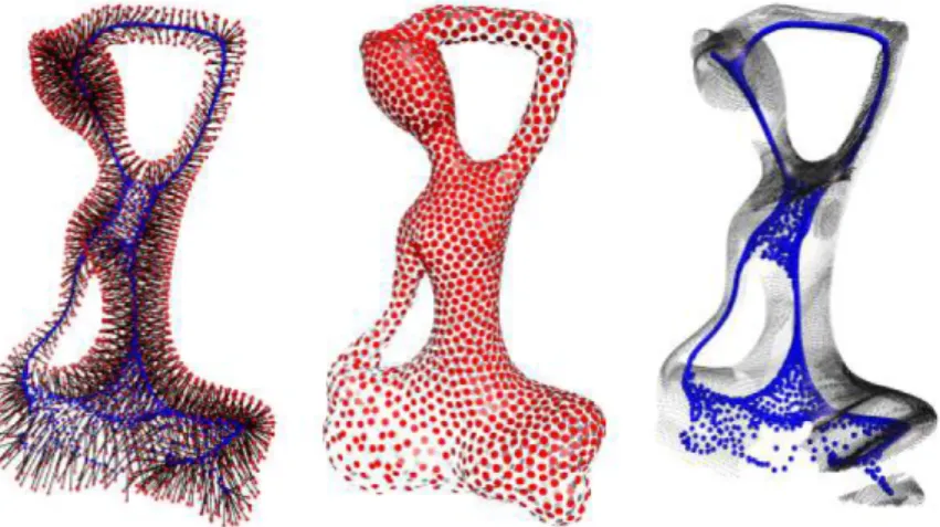
Figure 3.1: The deep points representation (left) is a set of line sec-tions, each with one end (red) on the surface (middle) and the other (blue) on the meso-skeleton (right).

augmented points,deep points, ordpointsfor short. See Figure3.1for an illustration of the deep points representation. The deep points for-m a sfor-mooth for-mapping between the surface and for-meso-skeleton, where their orientations agree with their corresponding surface normal direc-tions. It is worth noting that unlike the MAT, dpoints can be computed robustly from noisy and highly incomplete input.

The deep points representation is a result of an optimization ap-plied to the raw input point set. The key idea is to jointly optimize the surface and skeletal points so they form a valid deep points set. As we will show, the optimization converges where the inner points form a meso-skeleton, and the surface points are consolidated. The strength of the dpoints representation stems from the fact that it is comprised of both local and non-local geometric information. We demonstrate the advantages of dpoints by employing them to consolidate and com-plete noisy point clouds with large missing parts.

(49)

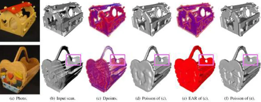
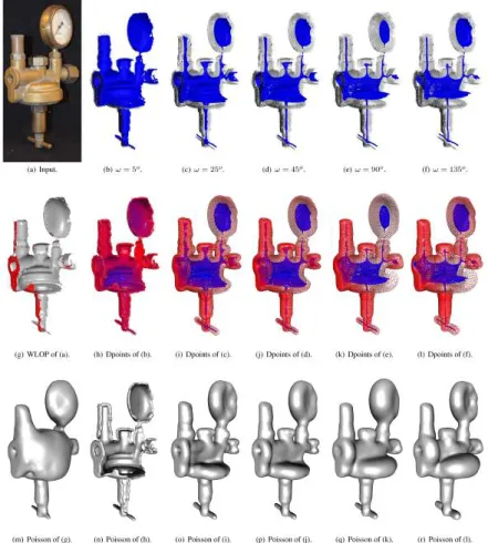
reconstruc-3.1. INTRODUCTION 39 tion. Advanced consolidation techniques [46,102,165,59,15] that can deal well with artifacts such as noise, outliers, irregular sampling, and sharp features rely on the availability of accurate normals. How-ever, vector normals as a second order differential feature remain noisy, especially near open boundaries. Thus, unreliable normals make it challenging to complete missing surface data in the proximity of boundary points. Our consolidation technique can complete the surface without assuming the availability of accurate surface normals. Figure3.2illustrates the main benefits of surface reconstruction using our dpoints representation. The raw scan in Figure 3.2(a) is non-uniform, many regions are sparse, and large parts are completely missing. Consequently, boundaries are not clearly defined and normal data is unreliable. Our dpoints representation computes a topological-ly correct meso-skeleton for the input shape, which provides non-local geometric information and guides the completion of missing regions on the surface. The result of our consolidated point set surface is shown in Figure3.2(e), to which we apply Poisson reconstruction in Figure3.2(f); see also the accompanying video.

In contrast, directly applying state-of-the-art reconstruction meth-ods to the noisy and incomplete input, such as Poisson reconstruc-tion [71] in Figure 3.2(b), does not provide plausible results. The WLOP technique [85, 57] excels in that it can consolidate raw and imperfect data without relying on normals. However, WLOP does not complete missing regions as is obvious in Figures3.2(c-d).

It should be noted that surface completion is, by its nature, an ill-posed problem. We therefore guide it by a coherent meso-skeleton, resulting in natural-looking reconstructions even for highly incom-plete scans; see an evaluation in Figure3.17. Furthermore, our com-pletion is contextual as it extrapolates the existing surface, rather than completing it with context-oblivious data, like circular [132] or elliptical [58] cross sections; see comparisons in Figure3.13.

The rest of this chapter is organized as follows: we discuss the background and previous work in Section3.2.

(50)

40 CHAPTER 3. DEEP POINTS CONSOLIDATION

(a) (b) (c) (d) (e) (f)

Figure 3.2: The input point cloud (a) contains noise and large missing regions. Applying Poisson surface reconstruction [71] on either the input (a) or the WLOP consolidation [57] result (c) does not yield satisfactory models; see (b) and (d), respectively. The surface points shown in (e) are consolidated and completed by our dpoints tech-nique. This leads to a much better Poisson surface reconstruction (f). In (c) and (e), the errors of the surface point normals estimated by local PCA are evaluated based on the ground truth and color coded (blue means higher error).

3.2

Related work

Surface reconstruction. In a broader context, our work is related

to the vast literature on surface reconstruction [55,139, 3]. Noise is a major challenge in handling real scanned data. Assuming local smoothness, methods based on signed distance functions (SDF) [18,

70,71] can reconstruct watertight surfaces. These techniques assume the whole model is scanned and when missing data is significant the reconstructed surfaces are often overly smooth and may contain topological errors. Please refer to Berger et al. [10,12] for a more comprehensive survey of state-of-the-art methods.

Surface Consolidation. Consolidation is an important

(51)

regu-3.2. RELATED WORK 41 larization, which works directly on a point set itself. Early work by [2] defines a point set surface through moving least squares (MLS) pro-jection. Later works focus on remitting the over-smoothing problem. Representative approaches include anisotropic smoothing [78], point-sampled cell complexes [1], algebraic point set surfaces [46], robust implicit MLS [102] and point set resampling [59]. To preserve sharp features, Avron et al. [7] use a`1-sparse method to compute piece-wise smooth surfaces, whereas Huang et al. [59] generate piecewise smooth point set surfaces through point projection. Recent work by Calderon and Boubekeur [15] preserves sharp features under a point morphology framework. All of these techniques depend on oriented normals for the projection control.

The most related work to our approach is Weighted Locally Opti-mal Projection (WLOP) [85,57], which generates a uniform distribut-ed point set with orientdistribut-ed normals. Preiner et al. [107] develop an accelerated version of WLOP by using a more compact representa-tion of the original input points. WLOP-based consolidarepresenta-tion methods are robust since they do not rely on the normals of the input points. However, none of them was designed to complete point clouds. In that sense, our method fuses consolidation and completion into one coherent technique.

Completion. Missing data, caused by self-occlusion, light

absorp-tion, or challenging surface materials [155], is one of the most chal-lenging problems in surface reconstruction. Diffusion-based method-s [28] are able to fill small holes with complex boundaries. To fill large holes, context-based [122,48], and repetition-based [165] methods are proposed, with the assumption that the missing parts can be re-placed with other parts of the input itself. Other methods infer missing data through exploiting high-level knowledge and priors, such as sym-metry relationships [103], volumetric smoothness [131], canonical regularities [82], and global parity measurement [121]. Nevertheless, these techniques cannot avoid erroneous topological reconstruction-s. Hence, interactive methods were developed to allow guiding the reconstruction with topology control [124,159].

(52)

42 CHAPTER 3. DEEP POINTS CONSOLIDATION (a) Input C (b) Initial consolidation S Sink Copy Joint optimization

(c) Forming the meso-skeleton Q

(d) Consolidating surface points P

(e) Dpoints

< <

P,Q

Figure 3.3: Deep points consolidation. Given the input point cloud (a) and its initial consolidation results (b), our approach creates deep points by sinking the inner points to form a meso-skeleton (c) and moving the outer points along the surface to complete missing areas (d). The final representation consists of a set of coherent vectors that connects the surface with the meso-skeleton.

Skeletonization. Skeletonization has been intensely studied in

com-puter graphics, e.g., [6,17,14,98]. In particular, curve skeleton tech-niques were developed in the context of surface reconstruction [123,

132, 81, 87,58]. Tagliasacchi et al. [132] introduce a curve skele-ton extraction mechanism by the use of the rotation symmetry axis. Huang et al. [58] computeL1-medial skeletons with conditional reg-ularization.

The work of Tagliasacchi et al. [129] computes meso-skeletons, which combine medial sheets and curve skeletons. We adapt their notion of meso-skeletons. However, our method differs in that we do not assume having a complete surface with reliable normals. We generate the meso-skeleton as a by-product of the point cloud consol-idation from noisy and incomplete input that lacks reliable normals. Miklos et al. [94] introduce a generalization of the MAT that provides a medial representation at different levels of abstraction. While this approach is more robust to noise, it still does not address the issue of incomplete data.

(53)

3.3. DEEP POINTS 43 these methods [132, 58] typically run cross-sectional curve interpo-lation and assume that the geometry of the cross-sectional curve is circular or elliptical. Our approach for computing meso-skeletons is inspired by the skeletonization scheme of [58]. However, we intro-duce new adaptive and anisotropic neighborhoods (Figure3.5), which allow us to generate skeletons of different topologies (2D sheets & 1D curves) under the same framework.

3.3

Deep Points

A deep point consists of a pair of pointshpi, qii, an outer pointpi∈R3

that resides on the surface and a corresponding inner pointqi ∈R3

that resides on a meso-skeleton. We refer to the outer points P =

{pi}i∈I as surface points and the inner onesQ={qi}i∈I as skeletal points, where the index set I is the same. We represent points in space and their orientations as column vectors, and denote orientation vectors with bold fonts.

The deep points representationhP, Qi={hpi, qii}i∈I ⊂R6shall

satisfy the following criteria:

• the surface pointsP reside on the latent surface and are regu-larly distributed;

• the collection of the skeletal pointsQforms a meso-skeleton of the surface, which may consists of both 2D surface sheets and 1D curves;

• the dpoint orientationmi= (pi−qi)/kpi−qikagrees with the surface normalniat the corresponding surface pointpi. These objectives yield a joint optimization of the surface and the skeletal points under both positionand orientation constraints. As the optimization converges, the deep points are generated.

We provide an overview of our algorithm in Figure 3.3. Let us denote the input point cloud withC={cj}j∈J ⊂R3(Figure3.3(a)).

(54)

44 CHAPTER 3. DEEP POINTS CONSOLIDATION may have large missing parts. We start by applying WLOP consolida-tion [57] onCto yield a denoised, oriented, and downsampled point setS ={si,ni}i∈I (Figure3.3(b)). Through replicating the consoli-dated inputSand sinking these replicated points down into the shape interior (Section3.4.1), an initial meso-skeleton (Figure3.3(c), left) is formed. We refer to points on this initial meso-skeleton as anchor points and denote them byH ={hi}i∈I.

With set S serving as the initial surface points (Figure 3.3(d), left) and set H serving as the initial skeletal points, we optimize the set hS, Hi(Figure 3.3(d) and (c), left to right) to form a valid deep points representation that satisfies the three criteria introduced above. In Section3.4.2, we describe the optimization of the skeletal points into a connected and topologically correct meso-skeleton of the surface. The corresponding surface point consolidation is presented in Section 3.4.3. We show a sequence of optimized point clouds in Figure3.3(c) and (d), including both skeletal and surface point sets, to demonstrate how this joint optimization converges to a valid state of deep pointshP, Qias presented in Figure3.3(e).

3.4

Joint Optimization on Dpoints

The joint optimization of dpoints consists of three stages: sinking the consolidated points S (Figure 3.3(b)) to obtain a set of anchor points H (Figure3.3(c), left), and then consolidating these anchor points H to form a meso-skeleton (Figure3.3(c), left to right), and finally consolidating a second copy of the surface pointsSto complete the missing areas and refine the connection to the meso-skeleton (Figure3.3(d), left to right). At the end, a good dpoints representation is obtained, which consists of a meso-skeleton with proper topology, a complete and consolidated point set surface, and an one-to-one mapping between the two, where the mapping (dpoint) orientation agrees with the surface normal (Figure3.3(e)).

(55)

3.4. JOINT OPTIMIZATION ON DPOINTS 45

3.4.1

Sinking Consolidated Points

Our algorithm to obtain an initial meso-skeleton is loosely inspired by the grassfire transform for binary images. Intuitively, we set the consolidated points “on fire”, causing the fire to burn from the surface into the volume of the shape. When opposing fire fronts meet, they stop propagating and form the initial meso-skeleton. We consider points that have met an opposing front as “anchored”. A key challenge in this step is that we work with point sets that may have large missing parts, i.e., are not closed, which may lead to regions that never meet an opposing front. We handle this problem by exploiting the dpoints representation, that is, the connection between moving inner points and their corresponding surface points.

We initialize outer and inner points of each dpointhpi, qiiby plac-ing both at the correspondplac-ing consolidated point si. This gives us dpoints of zero length, where the length means the distance between the outer and inner point. To move inner points into the volume of the shape and anchor them at proper locations, we apply an iterative pro-cedure. For each dpoint, we compute a static neighborhoodPion the surface points, and a dynamic neighborhoodQion the inner points, which we update at each iteration. We use the static neighborhood to determine the amount of movement into the volume for each inner point, and to maintain smoothness among neighboring inner points. On the other hand, we use the dynamic neighborhoods to determine whether opposing fronts meet and inner points settle.

In a preprocessing step, we first compute the average sparsityrof the consolidated point setS. That is,ris the average distance to the closest neighbor, r= 1 |S| X i∈I min i0_∈_I_\{_i_}ksi−si 0k, (3.1)

where operator k · kcomputes the Euclidean norm of a vector and

| · |measures the size of a set. We compute the static neighborhood

Pi = {pi0| kp_i0 −p_ik < σ_pr} for each surface point p_i where the

parameterσpdefaults to5, and denote its set index (the set of indices belonging toPi) byI_iP.

(56)

46 CHAPTER 3. DEEP POINTS CONSOLIDATION Within each iteration, we compute the dynamic neighborhood

Qi = {qi0| kq_i0 −q_ik < σ_qr} with the parameterσ_q = 2 by default,

and denote a set indexI_iQfor each inner pointqi. We use this neigh-borhood to detect whether an inner point qi should settle. We say opposing fronts meet within the dynamic neighborhood if

max i0_∈_IQ

i

ni0·n_i≤cos(ω), (3.2)

whereniare the normals of surface points, which we obtained in the initial consolidation step [57]. Intuitively, the above condition means that an inner point stops sinking once it meets other inner points with sufficiently different normals. The criteria for being sufficie