ISSN 1440-771X
Australia
Department of Econometrics and Business Statistics
http://www.buseco.monash.edu.au/depts/ebs/pubs/wpapers/
August 2007
Working Paper 11/07
A Bayesian Approach to Bandwidth Selection for
Multivariate Kernel Regression with an Application to
State-Price Density Estimation
A Bayesian Approach to Bandwidth Selection for Multivariate Kernel
Regression with an Application to State-Price Density Estimation
Xibin Zhang, Robert D. Brooks, and Maxwell L. King1 Department of Econometrics and Business Statistics, Monash University, Australia
August 2007
Abstract: Multivariate kernel regression is an important tool for investigating the relationship between a response and a set of explanatory variables. It is generally accepted that the perfor-mance of a kernel regression estimator largely depends on the choice of bandwidth rather than the kernel function. This nonparametric technique has been employed in a number of empiri-cal studies including the state-price density estimation pioneered by A¨ıt-Sahalia and Lo (1998). However, the widespread usefulness of multivariate kernel regression has been limited by the dif-ficulty in computing a data-driven bandwidth. In this paper, we present a Bayesian approach to bandwidth selection for multivariate kernel regression. A Markov chain Monte Carlo algorithm is presented to sample the bandwidth vector and other parameters in a multivariate kernel regres-sion model. A Monte Carlo study shows that the proposed bandwidth selector is more accurate than the rule-of-thumb bandwidth selector known as the normal reference rule according to Scott (1992) and Bowman and Azzalini (1997). The proposed bandwidth selection algorithm is applied to a multivariate kernel regression model that is often used to estimate the state-price density of Arrow-Debreu securities. When applying the proposed method to the S&P 500 index options and the DAX index options, we find that for short-maturity options, the proposed Bayesian band-width selector produces an obviously different state-price density from the one produced by using a subjective bandwidth selector discussed in A¨ıt-Sahalia and Lo (1998).
Key words: Black-Scholes formula, likelihood, Markov chain Monte Carlo, posterior density.
JEL Classification: C11, C14, G12
1Corresponding author. Email: [email protected]; telephone: +61-3-99052449.
1 Introduction
The multivariate kernel regression technique helps investigate the relationship between a response and a set of explanatory variables without imposing any parametric assumptions of the form of such a relationship. Stanton (1997) indicated that one potentially serious problem with any parametric model, particularly when we have no economic reason to prefer one functional form over another, is misspecification, which was further addressed by Backus, Foresi and Zin (1995) by showing that misspecification of interest rate models can lead to serious pricing and hedging errors2. However, A¨ıt-Sahalia and Lo (1998) indicated that the use of relevant nonparametric techniques often helps avoid misspecification problems caused by most parametric models.
In empirical studies, the multivariate kernel regression technique can be employed to avoid having to specify a functional form for the relationship between a response and a set of explanatory variables, which we denote asyandx= (x1, x2, . . . , xd)0, respectively. Given observations (yi,xi),
for i= 1,2,· · ·, n, the multivariate kernel regression model is expressed as
yi =m(xi) +εi, (1)
where εi, for i= 1,2,· · ·, n, are assumed to be independent and identically distributed (iid) with
mean zero and variance σ2
m. The Nadaraya-Watson estimator ofm(·) is given by
ˆ m(x,h) = n−1 Pn i=1Kh(x−xi)yi n−1Pn j=1Kh(x−xj) , (2)
where h= (h1, h2,· · ·, hd)0 is a vector of bandwidths with all elements positive, and
Kh(x) = 1 h1h2· · ·hd K µx 1 h1 ,x2 h2 ,· · ·,xd hd 
2Stanton (1997) also indicated that existing parametric models of interest rates do not even fit historical data
well. A¨ıt-Sahalia (1996) presented empirical studies to compare the marginal density implied by each parametric model with that estimated directly from the same data, and found that every parametric model of the spot rate previously proposed in the literature was rejected.
with K(·) denoting a multivariate kernel function. The nonparametric regression technique has been widely used in the empirical finance literature (see, for example, A¨ıt-Sahalia and Lo, 1998, 2000; Broadie, Detemple, Ghysels and Torres, 2000; A¨ıt-Sahalia, Bickel and Stoker, 2001; Breitung and Wulff, 2001; Mancuso, Goodwin and Grennes, 2003; Fernandes, 2006).
As the denominator of (2) is the kernel density estimator of f(x), the Nadaraya-Watson estimator of m(x) can be also expressed as (H¨ardle, 1990)
ˆ m(x,h) = 1 n n X i=1 wh,i(x)yi, (3) where wh,i(x) =Kh(x−xi)/fˆh(x), ˆ fh(x) = 1 n n X j=1 Kh(x−xj).
This indicates that the multivariate kernel regression estimator given by (2) is a weighted average of the observed values of y. Herrmann (2000) indicated that the region of such a local average and the amount of smoothness of the regression estimator are dominated by the bandwidth, and that the performance of kernel regression estimators largely depends on the choice of bandwidth rather than the kernel function. Multivariate kernel regression is an important technique for investigating the relationship between a response and covariates and has a number of important applications (Donald, 1997; Stanton, 1997; A¨ıt-Sahalia and Lo, 1998; Boudoukh, Whitelaw, Richardson and Stanton, 1997; among others). However, its widespread usefulness has been limited by the difficulty in deriving data-driven bandwidths. We remedy this deficiency in this paper.
According to H¨ardle and M¨uller (2000), methods employed for choosing a bandwidth in kernel regression are basically the same as those employed in kernel density estimation. A large body of literature exists on bandwidth selection for univariate kernel density estimation (see
Marron, 1987; Scott, 1992; Wand and Jones, 1995; Jones, Marron and Sheather, 1996; for surveys). However, the literature on bandwidth selection for multivariate kernel density estimation is quite limited. Sain, Baggerly and Scott (1994) employed the biased cross-validation method to estimate bandwidths for bivariate kernel density estimation. Wand and Jones (1994) and Duong and Hazelton (2003) presented plug-in algorithms for choosing bandwidths for bivariate data. However, the above-mentioned biased cross-validation method and plug-in algorithms cannot be directly extended to kernel density estimation with more than two variables (see, for example, Zhang, King and Hyndman, 2006). Hence there is little guidance in the literature on how to derive a data-driven bandwidth vector for multivariate kernel regression with more than two regressors, which is definitely an important issue in empirical studies.
Fan and Gijbels (2000) presented a survey on bandwidth selection for univariate local polyno-mial fitting, which includes the Nadaraya-Watson estimator as a special case. They discussed two bandwidth selectors, namely the rule-of-thumb and the plug-in bandwidth selectors, in which the former is basically the same as the rule-of-thumb bandwidth selector, also known as the normal reference rule (NRR) for kernel density estimation documented in Scott (1992) and Bowman and Azzalini (1997). NRR is often used in practice, in the absence of any other practical bandwidth selectors, even though lots of interesting data are non-Gaussian and sometimes kernel functions are not the Gaussian kernel. Herrmann, Wand, Engel and Gasser (1995) provided a detailed discussion of the bivariate plug-in bandwidth selector. However, the plug-in bandwidth selector cannot be directly extended to kernel regression with more than two regressors. The rule-of-thumb bandwidth selector is eligible for multivariate kernel regression in the situation, where the data are observed from a multivariate normal density and the kernel function is the standard normal density. This is a rather crude bandwidth selector, even though it is often used in practice, in the absence of any other practical bandwidth selectors, despite the fact that most interesting data are
non-Gaussian.
H¨ardle and M¨uller (2000) discussed bandwidth selection for multivariate kernel regression and showed that in practice, the cross-validation method is often employed to choose a data-driven bandwidth for kernel regression. This bandwidth selection method requires a numerical optimiza-tion procedure, which becomes increasingly difficult to implement as the number of regressors increases. Zhang, King and Hyndman (2006) presented a Bayesian approach to bandwidth selec-tion for multivariate kernel density estimaselec-tion, where bandwidths are treated as parameters, whose posterior is derived via the Kullback-Leibler information measure. In the context of choosing a data-driven bandwidth vector for multivariate kernel regression, we can also treathas a vector of parameters, whose posterior density can be obtained through the cross-validation method with a known distribution of errors given in (1). A posterior estimate of h can be derived via a Markov chain Monte Carlo (MCMC) algorithm. One important advantage of the MCMC technique for deriving a data-driven bandwidth vector (or matrix) is that it is applicable to data with any number of regressors. Moreover, the sampling algorithm involves no increased difficulty when the number of regressors increases.
The empirical finance literature is characterized by a number of problems that start with the state-price density (SPD) or pricing kernel implicit in the prices of traded financial assets. Major applications of this approach have focused on option pricing (A¨ıt-Sahalia and Lo, 1998; Broadie, Detemple, Ghysels and Torres, 2000; A¨ıt-Sahalia and Duarte, 2003; among others), value-at-risk estimation (see, for example, A¨ıt-Sahalia and Lo, 2000), modelling financial crashes (Fernandes, 2006; among others), modelling exchange rate dynamics (Brandt and Santa-Clara, 2002; Inci and Lu, 2004; among others), portfolio performance measurement (see, for example, Ayadi and Kryzanowski, 2005) and the term structure of interest rates (Hong and Li, 2005). Yatchew and
H¨ardle (2006) indicated that in general that economic theory does not propose specific functional forms for the state price densities. As such, Yatchew and H¨ardle (2006) proposed a nonparametric solution based on constrained least squares and a bootstrap procedure.
One important application of multivariate kernel regression is the one pioneered by A¨ıt-Sahalia and Lo (1998), who employed this nonparametric technique to estimate the SPD of Arrow-Debreu securities known as the fundamental building block for analyzing economic equilibrium under uncertainty. A¨ıt-Sahalia and Lo (1998) showed that in a dynamic equilibrium model, the price of a security is given by Pt= exp{rt,ττ}Et∗[Z(ST)] = exp{rt,ττ} Z ∞ −∞Z(ST)f ∗ t(ST)dST,
where T=t+τ, τ is the time to maturity, E∗
t represents the conditional expectation given
infor-mation available at date t,Z(ST) is the payoff of the security at date T, rt,τ is a constant risk-free
interest rate between t andT, and f∗
t(ST) is the date-t SPD for the payoff of the security at date
T. A¨ıt-Sahalia and Lo (1998) argued that the SPD summarizes all relevant information for the purpose of pricing the underlying security. When the underlying security is an option, A¨ıt-Sahalia and Lo (1998) indicated that the SPD is the second-order derivative of a call option-pricing for-mula with respect to strike price computed atST, and the option-pricing formula can be estimated
using the multivariate kernel regression technique.
A¨ıt-Sahalia and Lo (1998) argued that the price of a call option is a nonlinear function of (St, Xt, τ, rt,τ, δt,τ)0 with unknown form, in which δt,τ represents the dividend rate at datet. Once
the nonlinear relationship is estimated through the multivariate kernel regression technique, the second-order derivative of H with respect to X can be derived. This nonparametric approach to SPD estimation pioneered by A¨ıt-Sahalia and Lo (1998) has been followed in a large number of empirical studies, including Huynh, Kervella and Zheng (2002) who presented two methods for
dimension reduction.
A¨ıt-Sahalia and Lo (1998) presented comprehensive simulation and empirical studies to illus-trate the effectiveness of the multivariate kernel regression technique in estimating SPDs. However, it appears that their bandwidth vectors were chosen subjectively. As the choice of bandwidth plays an important role in multivariate kernel regression, we remedy this problem using a modification of Zhang, King and Hyndman’s (2006) algorithm for choosing data-driven bandwidths.
This paper aims to investigate the problem of choosing a data-driven bandwidth vector for multivariate kernel regression, where the bandwidth vector is treated as a vector of parame-ters. An algorithm will be presented to sample parameters from their posterior according to the Metropolis-Hastings rule, and the estimated bandwidth vector is optimal with respect to the av-eraged squared error (ASE) criterion, which will be further discussed in the next section. To the best of our knowledge, this algorithm represents the first data-driven bandwidth selection method for multivariate kernel regression with more than two regressors.
The rest of the paper is organized as follows. Section 2 provides a Bayesian approach to bandwidth selection for multivariate kernel regression models. In Section 3, we present a brief description of the nonparametric state-price density estimation method presented by A¨ıt-Sahalia and Lo (1998). In addition, we show how the Bayesian bandwidth selection technique can be ap-plied to the nonparametric estimation of volatility. A Monte Carlo study is presented to illustrate the accuracy of the proposed Bayesian bandwidth selector. Section 4 provides an application of the Bayesian bandwidth selection technique to volatility estimation and the state-price density estimation with S&P500 index options data and DAX index options data. Concluding remarks are given in the last section.
2 Bayesian Bandwidth Selector
2.1 Cross-validation
As we discussed in the previous section, the most important issue of multivariate kernel regression is the selection of the optimal bandwidth under a chosen criterion. One of such criteria is ASE given by ASE(h) = 1 n n X i=1 [ ˆm(xi,h)−m(xi)]2, (4)
and an optimal bandwidth, denoted by ˆho, is the one that minimizes ASE(h). The goodness of
fit of the Nadaraya-Watson estimator ˆm(xi,h) can be assessed by the sum of squared residuals
SSE(h) = 1 n n X i=1 [yi−mˆ(xi,h)]2, (5)
which is referred to as the re-substitution estimate of ASE by H¨ardle and M¨uller (2000). SSE(h) can be made arbitrarily small by allowing h −→ 0, because yi is used in ˆm(xi,h) to predict
itself. The cross-validation method involves estimating m(x) using data with the ith observation deleted, and the resultant leave-one-out estimator is
ˆ m−i(xi,h) = 1 (n−1) ˆfh(xi) n X j=1 j6=i Kh(xi−xj)yj, (6)
fori= 1,2,· · ·, n. An optimal bandwidth under the cross-validation rule is the one that minimizes CV(h) =
n
X
i=1
[yi−mˆ−i(xi,h)]2. (7)
Let ˆhcv denote the bandwidth obtained through cross-validation. H¨ardle, Hall and Marron (1988)
showed that ASE(ˆho)/ASE(ˆhcv)−→ 1 and ˆhcv −→hˆo, as n −→ ∞, where the convergence is in
probability. Hence ˆhcv is asymptotically optimal with respect to the ASE criterion.
Generally speaking, solving the problem of minimization of CV(h) with respect tohrequires a procedure of numerical optimization, which becomes increasingly difficult as the dimension of x
increases. However, if we treath as a vector of parameters, choosing bandwidths for multivariate kernel regression is equivalent to estimating parameters based on available data. When the errors in (1) are assumed to follow a known distribution, the likelihood of (y1, y2,· · ·, yn)0 given h can
be derived through the cross-validation method. Moreover, assuming prior densities for h, we can derive the posterior density of hup to a normalizing constant.
2.2 Likelihood
We consider the multivariate kernel regression model given by (1), where we assume that εi, for
i= 1,2,· · ·, n, are iid and follow N(0, σ2
m) with σ2m an unknown parameter.3 It follows that
yi−m(xi)
σm
iid∼N(0,1),
for i= 1,2,· · ·, n. Unfortunately the parametric form of m(xi) is unknown, so we consider using
the Nadaraya-Watson estimator given by (2) to replace m(xi). Thus introducing (h0, σm2)0 as a
vector of unknown parameters leads to an approximate likelihood of (y1, y2,· · ·, yn)0 as
l∗(y 1, y2,· · ·, yn|h, σ2m) = (2πσm2)−n/2exp ( − 1 2σ2 m n X i=1 (yi−mˆ(xi,h))2 ) . (8)
Unfortunately if we use this likelihood to optimize with respect to h, we end up with the trivial result that ˆm(xi,h) is arbitrarily close toyi by allowinghto approach zero. The standard solution
to this problem as noted above is to replace ˆm(xi,h) with the leave-one-out estimator ˆm−i(xi,h)
given by (6). We therefore propose
l(y1, y2,· · ·, yn|h, σm2) = (2πσm2)−n/2exp ( − 1 2σ2 m n X i=1 (yi−mˆ−i(xi,h))2 ) , (9)
3It should be noted that the distribution of errors given in (1) is not restricted to the assumption of iid normal.
The errors can be assumed to follow any known distribution or to be correlated, as long as the likelihood can be derived. However, the focus of this paper is to investigate estimating bandwidth rather than selecting an appropriate assumption for the errors. We will investigate this issue elsewhere.
as a likelihood of (y1, y2,· · ·, yn)0. As indicated by H¨ardle, Hall and Marron (1988), most
band-width selectors are based on the minimization of some functions of h which is related to SSE(h), and the minimizers of such functions are asymptotically optimal. Thus, ˆm(xi,h) and ˆm−i(xi,h)
are asymptotically equivalent in terms of choosing the optimal bandwidth. It is important to note that if σ2
m is kept as a constant, the cross-validation criterion for
choosing bandwidths for a multivariate kernel regression model is equivalent to the maximization of the likelihood function given by (9) with respect to h.
2.3 Posterior Estimate of the Bandwidth Vector
Let π(h) and π(σ2
m) denote the prior densities of h and σm2, respectively. According to Bayes
theorem, the posterior of (h0, σ2
m)0 is
π(h, σ2
m|y1, y2,· · ·, yn)∝π(h)π(σm2 )l(y1, y2,· · ·, yn|h, σ2m). (10)
Assume that the prior density of σ2
m is an inverted Gamma density denoted as IG(p/2, ν/2) with
its density function given by
π(σ2 m)∝ Ã 1 σ2 m !p/2+1 exp ( −ν/2 σ2 m ) , (11)
where p and ν are hyperparameters. The prior density of hj is assumed to be
π(hj)∝
1 1 +λh2
j
, (12)
Then the posterior of (h0, σ2
m)0 becomes π(h, σ2 m|y1, y2,· · ·, yn)∝ d X j=1 π(hj) Ã 1 σ2 m !(n+p)/2+1 exp ( − Pn i=1(yi−mˆ−i(xi,h))2+ν 2σ2 m ) . (13)
After integrating out σ2
m from (13), we obtain the posterior of h expressed as
π(h|y1, y2,· · ·, yn) =
Z
π(h, σ2|y
∝ d X i=1 π(hj) 1 2 n X j=1 (yi−mˆ−i(xi,h))2+ ν 2 −(n+p)/2 . (14)
The random-walk Metropolis-Hastings algorithm can be employed to samplehwith the acceptance probability computed through (14), while σ2
m can be sampled directly from
σ2 m ∼IG Ã n+p 2 , 1 2 n X i=1 (yi−mˆ−i(xi,h))2+ ν 2 ! . (15)
The ergodic average or the posterior mean of h acts as an estimate of the bandwidth vector, and the posterior mean of σ2
m is an estimate ofσm2.
It is important to note that if we ignore the effect of the prior ofh, the cross-validation criterion for choosing h is equivalent to maximizing the posterior of h given by (14) with respect to h. In addition, bandwidths are sampled from their posteriors using the Metropolis-Hastings algorithm, which does not encounter the computational difficulty encountered in the numerical minimization of CV(h) as the dimension of hincreases. The proposed Bayesian bandwidth selection algorithm is applicable to multivariate kernel regression models of any number of regressors without imposing any increased complexity of the sampling algorithm.
Note that the likelihood function given by (9) is flat when the components of h are large. If we use uniform priors for the components of hand employ the random-walk Metropolis-Hastings algorithm to sample h, the update ofhoften has a negligible effect on the acceptance probability when the components of hare already large. The purpose of the priors given by (12) is to assign a small prior probability on the “problematic” region in the parameter space, where the likelihood function is flat. See, for example, Zhang, King and Hyndman (2006) for a detailed discussion.
2.4 A Monte Carlo Study
The purpose of this Monte Carlo investigation is to examine the accuracy of the proposed band-width selector in comparison with the NRR, which is the rule-of-thumb bandband-width selector in many empirical studies in the absence of a data-driven bandwidth selector. Consider the relationship between y and x1 and x2 given by
y= sin(2πx1) + 4(x2−0.5)2+ε, (16) where x1 and x2 follow the uniform distribution on (0,1) denoted as U(0,1), andε ∼N(0, σm2).
A sample was generated by drawing x1,t and x2,t independently from U(0,1) and εt from
N(0,0.5) and calculating yt according to (16), for t= 1,2,· · ·, n, where the sample size n is 1000.
The relationship betweenytand (x1,t, x2,t) can be approximated by a multivariate kernel regression
model given by
yt=m(x1,t, x2,t) +εt, (17)
for t = 1,2,· · ·, n, where the bandwidth was estimated through our Bayesian bandwidth selector and NRR, respectively. When a bandwidth was chosen, we calculated the fitted value of yt
according to (2), for t= 1,2,· · ·, n.
The accuracy of the chosen bandwidth is examined by the fitness measure given by
R2 = 1− Pn t=1(yt−yˆt)2 Pn t=1(yt−y)2 ,
where ˆyt is the fitted value of yt calculated through (17) with the chosen bandwidths, and y is
the mean of yt, for t= 1,2,· · ·, n. Note that the larger the value of R2 is, the more accurate the
The Monte Carlo procedure consists of 2000 iterations. The average value of R2 computed through our Bayesian bandwidth selector is 0.5619, which is higher than its counterpart of 0.5358 computed through NRR. In addition, we found that at each iteration of the Monte Carlo sim-ulation, the value of R2 derived through the our bandwidth selector is larger than that derived through NRR. We also calculated the difference between the values ofR2 computed, respectively, through our bandwidth selector and NRR. We found that the average and the standard deviation of such differences are 0.0262 and 0.007, respectively. Thus, the Monte Carlo study supports our Bayesian bandwidth selector against NRR according to the goodness-of-fit measure.
3 Nonparametric State-Price Density Estimation
3.1 SPD Estimator Derived via Black-Scholes Formula
A¨ıt-Sahalia and Lo (1998) discussed the relationship between the pricing of derivative securities and their SPDs. Let St represent the date-t price of an asset, pt the date-t price of a derivative
security written on the asset, and Z(ST) the date-T payoffs of the security. In a dynamic
equilib-rium model,ptcan be expressed as the expected net present value ofZ(ST), where the expectation
is computed in terms of the state-price density ft(ST). According to A¨ıt-Sahalia and Lo’s (1998)
discussion, SPD is sufficient for the purpose of asset pricing.
When the derivative security is an option, A¨ıt-Sahalia and Lo (1998) indicated that the SPD is proportional to the second-order derivative of a call option-pricing formula with respect to the strike price. Under the hypothesis of Black and Scholes (1973) and Merton (1973), the date-t
price of a call option maturing at date T is given by
where X is the strike price, σ is the volatility of the underlying asset, τ = T −t, Φ(·) is the Gaussian cumulative density function, and d1 and d2 are defined as
d1 =
ln(St/X) + (rt,τ −δt,τ +σ2/2)
σ√τ , and d2 =d1−σ
√ τ .
According to A¨ıt-Sahalia and Lo (1998) and Huynh, Kervella and Zheng (2002), the formula of the SPD and the risk measures of delta (∆) and gamma (Γ) are given by
fBS,t(ST) = 1 ST √ 2πσ2τ exp ( −[ln(ST/St)−(rt,τ −δt,τ−σ2/2)τ]2 2σ2τ ) , (18) ∆BS = ∂HBS(St, X, τ, rt,τ, δt,τ;σ) ∂St = Φ(d1), (19) ΓBS = ∂2H BS(St, X, τ, rt,τ, δt,τ;σ) ∂S2 t = φ(d1) Stσ √ τ, (20)
where φ(·) is the Gaussian density function.
3.2 Nonparametric Estimation of Option-Pricing Formula
A¨ıt-Sahalia and Lo (1998) argued that the SPD estimator given by (18) is associated with the parametric assumptions underlying the Black-Scholes option-pricing model. If any of these as-sumptions does not hold, option prices derived though (18) might be incorrect. A¨ıt-Sahalia and Lo (1998) showed that the date-t price of a call option, denoted by H, can be viewed as an unknown nonlinear function of z = (St, Xt, τ, rt,τ, δt,τ)0, which can be estimated through the multivariate
kernel regression technique. The Nadaraya-Watson estimator of the relation between H and z is given by ˆ H(z|h) = n−1 Pn i=1Kh(z−zi)Hi n−1Pn i=1Kh(z−zi) , (21)
where (Hi,zi), for i= 1,2,· · ·, n, are paired observations of (H,z).
As we discussed in previous sections, choosing a data-driven bandwidth under a chosen crite-rion is an important issue for multivariate kernel regression, which was emphasized by A¨ıt-Sahalia
and Lo (1998) though a graphical demonstration. They suggested choosing bandwidths according to the formula given by
hj =cjs(zj)n−1/(d+2p), (22)
for j = 1,2,· · ·, d, where pis the order of the kernel function, s(zj) is the unconditional standard
deviation of zj, andcj is a constant depending on the sample size kernel choices. This bandwidth
selector is similar to the rule-of-thumb bandwidth selector and seems to be somewhat subjective. However, we can employ our Bayesian approach to bandwidth selection for multivariate kernel regression discussed in Section 2 to derive a data-driven bandwidth.
A¨ıt-Sahalia and Lo (1998) raised a practical concern about the dimension involved in the multivariate kernel regression given by (21), because it is increasingly difficult to derive accurate estimators of the regression function and its derivatives as the number of regressors increases. They presented three methods to reduce the number of regressors, and one of these methods assumes that the call-option pricing formula is given by the Black-Scholes formula except that the date-t implied volatility, denoted by σt, is a nonparametric function of ˜z = (Ft, X, τ), where Ft is
the date-t futures price of the underlying asset. The kernel estimator of the regression function of
σ on ˜z is given by ˆ σ(Ft, X, τ|h˜) = n−1Pn i=1Kh˜( ˜z−z˜i)σi n−1Pn i=1K˜h( ˜z−z˜i) , (23)
whereσiis the volatility implied by the pricesHi, and ˜his a vector of bandwidths. The call-option
pricing function is given by ˆ H(St, X, τ, rt,τ, δt,τ) =HBS ³ St, X, τ, rt,τ, δt,τ; ˆσ(Ft, X, τ|h˜) ´ , (24)
based on which the option’s ∆, γ and SPD estimators can obtained by substituting ˆσ(Ft, X, τ|h˜)
A¨ıt-Sahalia and Lo (1998) demonstrated that the SPD derived through the above dimension-reduction method is not significantly different from that obtained through the full nonparametric regression model (21). In what follows, we will employ the Bayesian bandwidth selector presented in Section 2 to choose a data-driven bandwidth vector for the kernel estimator given by (23).
4 Applications of the Bayesian Bandwidth Selector
In order to investigate the empirical relevance of the Bayesian bandwidth selector for the kernel regression employed by A¨ıt-Sahalia and Lo (1998) for the purpose of estimating SPD, ∆ and Γ through the Black-Scholes formula, we apply the Bayesian bandwidth selector and its counterpart of NRR to the kernel regression with two data sets, the S&P 500 index options data and the DAX index options data.
4.1 S&P 500 Index Options Data
The data consist of n=14,431 observations of the implied volatility, futures price and time to maturity for the sample period from January 4, 1993 to December 31, 1993. A¨ıt-Sahalia and Lo (1998) demonstrated the empirical relevance of the kernel regression technique in estimating the SPD of S&P 500 index options price, where bandwidths were chosen using NRR and adjusted by some constants depending on the particular choices of kernels for the regressors. A¨ıt-Sahalia and Lo (1998) found obvious differences between the nonparametric SPD and the Black-Scholes SPD in a number of aspects, in particular, for all four maturities under investigation, the nonparametric SPDs are more negatively skewed and have thicker tails than the Black-Scholes SPDs, respectively. In addition, the amount of skewness and kurtosis both increase with maturity.
A¨ıt-Sahalia and Lo (1998) concluded that the SPD of the options price derived from the kernel regression of H on z are not significantly different from those computed from the Black-Scholes formula with volatility estimated by the kernel regression of σ on ˜z. The kernel regression model is given by
σt= ˜m( ˜zt) +εt, (25)
for t= 1,2,· · ·, n, where εt, for t= 1,2,· · ·, n, are assumed to be iid and distributed asN(0, σ2m).
The multivariate kernel function used by A¨ıt-Sahalia and Lo (1998) is the product of three uni-variate kernels, where the kernel function for futures price and time to maturity is
k(4)(x) = 1 √ 8π ³ 1−x2/3´exp(−x2/2), while the kernel for strike price is the Gaussian kernel.
When applying our Bayesian bandwidth selector to the multivariate kernel regression model given by (25), we chose the kernel function as the product of univariate Gaussian kernels. In order to obtain the closed form of the posterior density of (˜h0, σ2
m), we set the hyperparameters
as λ = 1, p= 2 and ν = 0.1, where the values of pand ν are quite standard in many algorithms for sampling the variance parameter (see, for example, Shephard and Pitt, 1997). We used the random-walk Metropolis-Hastings algorithm to sample ˜hfrom its posterior, whileσ2
m was directly
sampled from an inverted Gamma density given by (15). We employed the batch-mean standard error and the simulation inefficiency factor (SIF) to check the convergence performance of the sampling algorithm (see, for example, Roberts, 1996; Kim, Shephard and Chib, 1998; Tse, Zhang and Yu, 2004). Both the batch-mean standard error and SIF indicate that all the simulated chains have converged very well. Table 1 presents the estimated σ2
m and bandwidths, as well as their
To examine the sensitivity of prior choices for ˜h, we also employed a different prior given by π(hj)∝ 1−exp(−h2 j/2) exp(h2 j/2) , (26)
forj = 1,2,· · ·, d. In each iteration of the sampling procedure, such priors are able to prevent the updates of bandwidths from getting too large and too small. We found that the MCMC outputs are quite similar to those reported in Table 1. Thus, we found that the sampling algorithm is insensitive to difference choices of hyperparameters.
Using the bandwidths estimated respectively, through our Bayesian bandwidth selector and NRR, we computed the fitted values of σt through the nonparametric regression model given by
(23). After replacing σ with the fitted σt in (18) to (20), we calculated the estimates of SPD,
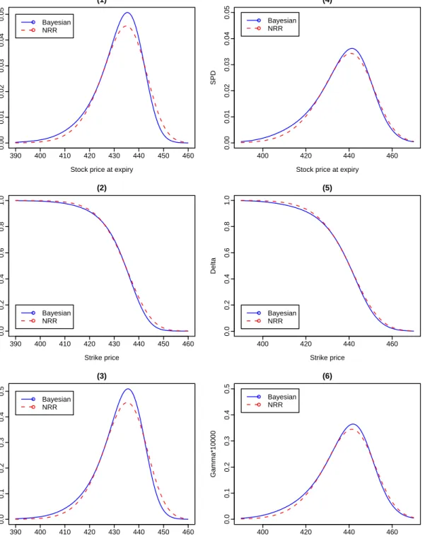
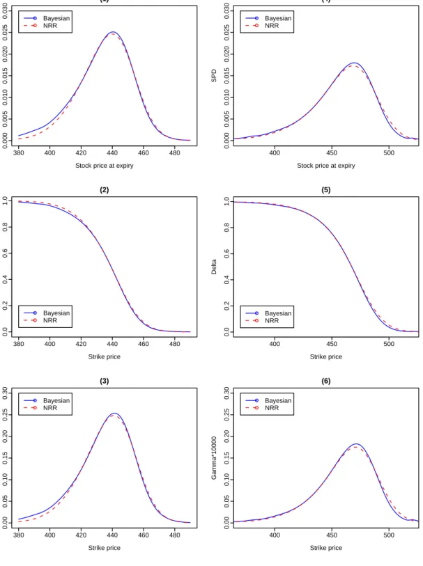
∆ and Γ at the tth observation, for t = 1,2,· · ·, n. The graphs of SPD, ∆ and Γ computed at different times to maturity are presented in Figures 1 and 2, where times to maturity were chosen to be 10, 25, 50 and 100 days, respectively. When time to maturity is short such as τ=10 days, we found that the SPD estimated through our Bayesian bandwidth selector has a thicker left tail and a thinner right tail than the SPD estimated through NRR, and that the former is more negatively skewed and has a higher peak than the latter. With time to maturity increasing, the differences between the SPDs estimated respectively, through the Bayesian bandwidth selector and NRR become less obvious.
Figures 1 and 2 reveal observable differences between the graphs of ∆ estimated respectively, through the Bayesian bandwidth selector and NRR, while such differences are almost unchanged as time to maturity increases. We found that the differences between the graphs of Γ estimated through the Bayesian bandwidth selector and NRR behave similarly to those between the graphs of SPD estimated through the two bandwidth selectors.
At any time to maturity under investigation, the SPDs estimated through the Bayesian band-width selector are more negatively skewed and have thicker tails than those estimated through NRR. Moreover, the peak of SPD estimated through the Bayesian bandwidth selector is higher than that estimated through NRR, even though the differences between the former and the latter become less obvious as time to maturity increases.
4.2 DAX Index Options Data
The data set contains 2972 daily settlement prices for each call-option contract of January 1997 (28 trading days) with the following variables: option price, spot price, strike price, time to maturity, risk-free interest rate, dividend, futures price and implied volatility. This data set was provided by Huynh, Kervella and Zheng (2002), who derived similar results as those reported by A¨ıt-Sahalia and Lo (1998).
When fitting the multivariate regression model of σt on (Ft, X, τ) given by (25) to the DAX
index options data, we chose the multivariate kernel to be the product of univariate Gaussian kernels, where the bandwidths were selected through our Bayesian bandwidth selector. The priors of bandwidths are given by (26) and the prior of σ2
m is given by (11) withp= 2 and ν= 0.1. The
random-walk Metropolis-Hastings algorithm was employed to sample ˜h from its posterior, while
σ2
m was sampled directly from the inverted Gamma density given by (15). The estimatedσm2 and
bandwidths, as well as their associated statistics are given in Table 2, where both the batch-mean standard error and SIF indicate that all the simulated chains have converged very well.
Using the bandwidths estimated through the Bayesian bandwidth selector, we calculated the fitted values ofσt according to the kernel regression model given by (23). With σ replaced by the
t = 1,2,· · ·, n. For comparison purposes, we also employed NRR for choosing the bandwidths, with which we derived the estimates of SPD, ∆ and Γ, respectively.
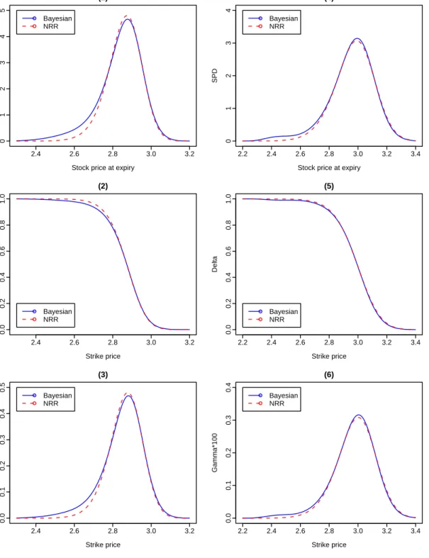
The graphs of SPD, ∆ and Γ computed at different times to maturity are provided in Figures 3 and 4. When time to maturity is short such as τ=10 days, we found that the SPD estimated through our Bayesian bandwidth selector has a thicker left tail than the SPD estimated through the NRR, while their right tails have no obvious differences. However, the graph of SPD estimated through the Baysian bandwidth selector is not obviously different from that estimated through NRR as time to maturity increases. Moreover, we found that the peak of SPD estimated through the Bayesian bandwidth selector is slightly lower than that estimated through NRR when τ=10 days, while the former is slightly higher than the latter when τ=25, 50 and 80 days.
Figures 3 and 4 show that the differences between the graphs of ∆ calculated through the Bayesian bandwidth selector and NRR is obvious when time to maturity is short such as τ=10 days, while such differences become less obvious as time to maturity increases. It was found from Figures 3 and 4 that the differences between the graphs of Γ estimated respectively, through the Bayesian bandwidth selector and NRR, behave similarly to those between the graphs of SPD estimated through the two bandwidth selectors.
To summarize the findings from both applications, we have found that for short-maturity options, the graphs of SPD and Γ estimated through our Bayesian bandwidth selector are respec-tively, different from those estimated through NRR, and that such differences become less obvious as time to maturity increases. Moreover, differences between the graphs of ∆ estimated through the two bandwidth selectors are also observed. As the Monte Carlo simulation study presented in Section 2.4 supports our Bayesian bandwidth selector against NRR, we recommend the use of our Bayesian bandwidth selector for the multivariate kernel regression involved in the nonparametric
estimation of SPD pioneered by A¨ıt-Sahalia and Lo (1998). The Bayesian bandwidth selector provides a data-driven solution to bandwidth selection for multivariate kernel regression models with any number of regressors.
5 Conclusion
This paper presents a Bayesian approach to bandwidth selection for multivariate kernel regression. To our knowledge, the proposed sampling algorithm represents the first data-driven method for choosing bandwidths for kernel regression with more than two regressors. A Monte Carlo study shows that the proposed bandwidth selector is more accurate than the normal reference rule, where the latter is often used in empirical studies in the absence of any other data-driven bandwidth selectors, despite the fact that most interesting data are non-Gaussian, and that sometimes kernel functions are not the Gaussian kernel. Our sampling algorithm provides a solution for choosing a data-driven bandwidth for multivariate kernel regression, which is employed for estimating the state-price density of Arrow-Debreu securities. When applying the proposed Baysian bandwidth selector to the kernel regression of implied volatility on the futures price, strike price and time to maturity, we have found that for short-maturity options, the estimated volatility produces an obviously different SPD from the one produced by using a subject bandwidth selector discussed in A¨ıt-Sahalia and Lo (1998). Our paper provides a data-driven solution for choosing bandwidths for the multivariate kernel regression involved in the nonparametric estimation of the state-price density pioneered by A¨ıt-Sahalia and Lo (1998).
An obvious extension of this study would be to investigate bandwidth selection for nonpara-metric multivariate local polynomial fitting, which A¨ıt-Sahalia and Duarte (2003) employed to estimate the state-price density under shape restrictions.
Acknowledgements
We would like to thank Yiu Kuen Tse for drawing our attention to this topic. We extend our sincere thanks to Yacine A¨ıt-Sahalia for providing constructive suggestions and the S&P500 options data, and Wolfgang H¨ardle and Kim Huynh for providing useful advice. We gratefully acknowledge computational support from the Victorian Partnership for Advanced Computing (VPAC) and financial support from the Australian Research Council under Discovery Project DP0664926.
References
A¨ıt-Sahalia, Y., 1996. Testing continuous-time models of the spot interest rate. Review of Finan-cial Studies 9, 385-426.
A¨ıt-Sahalia, Y., Lo, A.W., 1998. Nonparametric estimation of state-price densities implicit in financial asset prices. The Journal of Finance 53, 499-547.
A¨ıt-Sahalia, Y., Bickel, P., Stoker, T., 2001. Goodness-of-fit tests for kernel regression with an application to option implied volatilities. Journal of Econometrics 105, 363-412.
A¨ıt-Sahalia, Y., Duarte, J., 2003. Nonparametric option pricing under shape restrictions. Journal of Econometrics 116, 85-112.
A¨ıt-Sahalia, Y., Lo, A.W., 2000. Nonparametric risk management and implied risk aversion. Journal of Econometrics 94, 9-51.
Ayadi, M., Kryzanowski, L., 2000. Portfolio performance measurement using APM-free kernel models. Journal of Banking and Finance 29, 623-659.
Backus, D.K., Foresi, S., Zin, S.E., 1998. Arbitrage opportunities in arbitrage-free models of bond pricing. Journal of Business and Economic Statistics 16, 13-24.
Boudoukh, J., Whitelaw, R.F., Richardson, M., Stanton, R., 1997. Pricing mortgage-backed secu-rities in a multifactor interest rate environment: a multivariate density estimation approach. Review of Financial Studies 10, 405-446.
Bowman, A.W., Azzalini, A., 1997. Applied Smoothing Techniques for Data Analysis. Oxford University Press, London.
Brandt, M., Santa-Clara, P., 2002. Simulated likelihood estimation of diffusions with an appli-cation to exchange rate dynamics in incomplete markets. Journal of Financial Economics 63, 161-210.
Breitung, J., Wulff, C., 2001. Non-linear error correction and the efficient market hypothesis: the case of German dual-class shares. German Economic Review 2, 419-434.
Broadie, M., Detemple, J., Ghysels, E., Torres, O., 2000. American options with stochastic dividends and volatility: a nonparametric investigation. Journal of Econometrics 94, 53-92. Donald, S.G., 1997. Inference concerning the number of factors in a multivariate nonparametric
relationship. Econometrica 65, 103-131.
Duong, T., Hazelton, M.L., 2003. Plug-in bandwidth selectors for bivariate kernel density estima-tion. Journal of Nonparametric Statistics 15, 17-30.
Fan, J., Gijbels, I., 2000. Local polynomial fitting. In Schimek, M.G. (Eds.), Smoothing and Regression: Approaches, Computation, and Application. John Wiley & Sons, New York, 229-276.
Fernandes, M., 2006. Financial crashes as endogenous jumps: estimation, testing and forecasting. Journal of Economic Dynamics and Control 30, 111-141.
H¨ardle, W., 1990. Applied Nonparametric Regression. Cambridge University Press, London. H¨ardle, W., Hall, P., Marron, J.S., 2000. How far are automatically chosen regression estimators
from their optimum? Journal of the American Statistical Association 83, 86-97.
H¨ardle, W., M¨uller, M., 2000. Multivariate and semiparametric kernel regression. In Schimek, M.G. (Eds.), Smoothing and Regression: Approaches, Computation, and Application. John Wiley & Sons, New York, 357-392.
Herrmann, E., 2000. Variance estimation and bandwidth selection for kernel regression. In Schimek, M.G. (Eds.), Smoothing and Regression: Approaches, Computation, and Appli-cation. John Wiley & Sons, New York, 71-108.
Herrmann, E., Wand, M.P., Engel, J., Gasser, T., 1995. A bandwidth selector for bivariate kernel regression. Journal of the Royal Statistical Society Series B 57, 171-180.
Hong, Y., Li, H., 2005. Nonparametric specification testing for continuous-time models with applications to term structure of interest rates. Review of Financial Studies 18, 37-84.
Huynh, K., Kervella, P. Zheng, J., 2002. Estimating state-price densities with nonparametric re-gression. In H¨ardle, W., Kleinow, T., Stahl, G. (Eds.), Applied Quantitative Finance. Springer Verlag, Heidelberg, 171-196.
Inci, A., Lu, B., 2004. Exchange rates and interest rates: can term structure models explain currency movements. Journal of Economic Dynamics and Control 28, 1595-1624.
Jones, M.C., Marron, J.S., Sheather, S.J., 1996. A brief survey of bandwidth selection for density estimation. Journal of the American Statistical Association 91, 401-407.
Kim, S., Shephard, N., Chib, S., 1998. Stochastic volatility: likelihood inference and comparison with ARCH models. Review of Economic Studies 65, 361-393.
Mancuso, A., Goodwin, B., Grennes, T., 2003. Nonlinear aspects of capital market integration and real interest rate equalization. International Review of Economics and Finance 12, 283-303. Marron, J.S., 1987. A comparison of cross-validation techniques in density estimation. Annals of
Statistics 15, 152-162.
Roberts, G.O., 1996. Markov chain concepts related to sampling algorithms. In Gilks, W.R., Richardson, S., Spiegelhalter, D.J. (Eds.), Markov Chain Monte Carlo in Practice. Chapman & Hall, London, 45-57.
Sain, S.R., Baggerly, K.A., Scott, D.W., 1994. Cross-validation of multivariate densities. Journal of the American Statistical Association 89, 807-817.
Scott, D.W., 1992. Multivariate Density Estimation: Theory, Practice, and Visualization. John Wiley & Sons, New York.
Shephard, N., Pitt, M.K., 1997. Likelihood analysis of non-Gaussian measurement time series. Biometrika 84, 653-667.
Stanton, R., 1997. A nonparametric model of term structure dynamics and the market price of interest rate risk. The Journal of Finance 52, 1973-2002.
Tse, Y.K., Zhang, X., Yu, J., 2004. Estimation of hyperbolic diffusion using the Markov chain Monte Carlo simulation method. Quantitative Finance 4, 158-169.
Wand, M.P., Jones, M.C., 1994. Multivariate plug-in bandwidth selection. Computational Statis-tics 9, 97-116.
Wand, M.P., Jones, M.C., 1995. Kernel Smoothing. Chapman & Hall, London.
Yatchew, A., H¨ardle, W., 2006. Nonparametric state price density estimation using constrained least squares and the bootstrap. Journal of Econometrics 133, 579-599.
Zhang, X., King, M.L., Hyndman, R.J., 2006. A Bayesian approach to bandwidth selection for multivariate kernel density estimation. Computational Statistics and Data Analysis 50, 3009-3031.
Table 1: Estimated parameter and bandwidths with some statistics: S&P500 index options data
Parameters Mean Standard Batch-mean SIF Acceptance deviation standard error rate
σm 0.01076812 0.00006281 0.00000088 0.98 — ˜ h1 5.62857314 0.08345297 0.00310895 6.94 0.22 ˜ h2 5.47642603 0.10345975 0.00409019 7.81 0.20 ˜ h3 9.75492547 0.14585289 0.00599846 8.46 0.22
Table 2: Estimated parameter and bandwidths with some statistics: DAX index options data
Parameters Mean Standard Batch-mean SIF Acceptance deviation standard error rate
σm 0.01426562 0.00018372 0.00000140 1.16 — ˜ h1 1.53993302 0.99521769 0.02304122 10.72 0.27 ˜ h2 0.07667259 0.00316975 0.00007640 11.62 0.22 ˜ h3 0.02632898 0.00103973 0.00003053 17.24 0.22
Figure 1: The estimated SPD, ∆ and Γ based on S&P 500 index options data. The first column is for a maturity of 10 days, and the second column is for a maturity of 25 days.
390 400 410 420 430 440 450 460 0.00 0.01 0.02 0.03 0.04 0.05 (1)
Stock price at expiry
SPD Bayesian NRR 400 420 440 460 0.00 0.01 0.02 0.03 0.04 0.05 (4)
Stock price at expiry
SPD Bayesian NRR 390 400 410 420 430 440 450 460 0.0 0.2 0.4 0.6 0.8 1.0 (2) Strike price Delta Bayesian NRR 400 420 440 460 0.0 0.2 0.4 0.6 0.8 1.0 (5) Strike price Delta Bayesian NRR 390 400 410 420 430 440 450 460 0.0 0.1 0.2 0.3 0.4 0.5 (3) Strike price Gamma*10000 Bayesian NRR 400 420 440 460 0.0 0.1 0.2 0.3 0.4 0.5 (6) Strike price Gamma*10000 Bayesian NRR
Figure 2: The estimated SPD, ∆ and Γ based on S&P 500 index options data. The first column is for a maturity of 50 days, and the second column is for a maturity of 100 days.
380 400 420 440 460 480 0.000 0.005 0.010 0.015 0.020 0.025 0.030 (1)
Stock price at expiry
SPD Bayesian NRR 400 450 500 0.000 0.005 0.010 0.015 0.020 0.025 0.030 (4)
Stock price at expiry
SPD Bayesian NRR 380 400 420 440 460 480 0.0 0.2 0.4 0.6 0.8 1.0 (2) Strike price Delta Bayesian NRR 400 450 500 0.0 0.2 0.4 0.6 0.8 1.0 (5) Strike price Delta Bayesian NRR 380 400 420 440 460 480 0.00 0.05 0.10 0.15 0.20 0.25 0.30 (3) Strike price Gamma*10000 Bayesian NRR 400 450 500 0.00 0.05 0.10 0.15 0.20 0.25 0.30 (6) Strike price Gamma*10000 Bayesian NRR
Figure 3: The estimated SPD, ∆ and Γ based on DAX index options data. The first column is for a maturity of 10 days, and the second column is for a maturity of 25 days.
2.4 2.6 2.8 3.0 3.2 0 1 2 3 4 5 (1)
Stock price at expiry
SPD Bayesian NRR 2.2 2.4 2.6 2.8 3.0 3.2 3.4 0 1 2 3 4 (4)
Stock price at expiry
SPD Bayesian NRR 2.4 2.6 2.8 3.0 3.2 0.0 0.2 0.4 0.6 0.8 1.0 (2) Strike price Delta Bayesian NRR 2.2 2.4 2.6 2.8 3.0 3.2 3.4 0.0 0.2 0.4 0.6 0.8 1.0 (5) Strike price Delta Bayesian NRR 2.4 2.6 2.8 3.0 3.2 0.0 0.1 0.2 0.3 0.4 0.5 (3) Strike price Gamma*100 Bayesian NRR 2.2 2.4 2.6 2.8 3.0 3.2 3.4 0.0 0.1 0.2 0.3 0.4 (6) Strike price Gamma*100 Bayesian NRR
Figure 4: The estimated SPD, ∆ and Γ based on DAX index options data. The first column is for a maturity of 50 days, and the second column is for a maturity of 80 days.
2.0 2.5 3.0 3.5 0.0 0.5 1.0 1.5 2.0 2.5 (1)
Stock price at expiry
SPD Bayesian NRR 2.0 2.5 3.0 3.5 0.0 0.5 1.0 1.5 2.0 (4)
Stock price at expiry
SPD Bayesian NRR 2.0 2.5 3.0 3.5 0.0 0.2 0.4 0.6 0.8 1.0 (2) Strike price Delta Bayesian NRR 2.0 2.5 3.0 3.5 0.0 0.2 0.4 0.6 0.8 1.0 (5) Strike price Delta Bayesian NRR 2.0 2.5 3.0 3.5 0.00 0.05 0.10 0.15 0.20 0.25 (3) Strike price Gamma*100 Bayesian NRR 2.0 2.5 3.0 3.5 0.00 0.05 0.10 0.15 0.20 (6) Strike price Gamma*100 Bayesian NRR