March 2008, Volume 25, Issue 5. http://www.jstatsoft.org/
Text Mining Infrastructure in
R
Ingo Feinerer Wirtschaftsuniversit¨at Wien Kurt Hornik Wirtschaftsuniversit¨at Wien David Meyer Wirtschaftsuniversit¨at Wien AbstractDuring the last decade text mining has become a widely used discipline utilizing sta-tistical and machine learning methods. We present the tm package which provides a framework for text mining applications withinR. We give a survey on text mining facili-ties inRand explain how typical application tasks can be carried out using our framework. We present techniques for count-based analysis methods, text clustering, text classification and string kernels.
Keywords: text mining, R, count-based evaluation, text clustering, text classification, string kernels.
1. Introduction
Text mining encompasses a vast field of theoretical approaches and methods with one thing in common: text as input information. This allows various definitions, ranging from an extension of classical data mining to texts to more sophisticated formulations like “the use of large on-line text collections to discover new facts and trends about the world itself” (Hearst 1999). In general, text mining is an interdisciplinary field of activity amongst data mining, linguistics, computational statistics, and computer science. Standard techniques are text classification, text clustering, ontology and taxonomy creation, document summarization and latent corpus analysis. In addition a lot of techniques from related fields like information retrieval are commonly used.
Classical applications in text mining (Weisset al. 2004) come from the data mining commu-nity, like document clustering (Zhao and Karypis 2005b,a;Boley 1998;Boleyet al.1999) and document classification (Sebastiani 2002). For both the idea is to transform the text into a structured format based on term frequencies and subsequently apply standard data mining techniques. Typical applications in document clustering include grouping news articles or in-formation service documents (Steinbachet al.2000), whereas text categorization methods are
used in, e.g., e-mail filters and automatic labeling of documents in business libraries (Miller 2005). Especially in the context of clustering, specific distance measures (Zhao and Karypis 2004; Strehl et al. 2000), like the Cosine, play an important role. With the advent of the World Wide Web, support for information retrieval tasks (carried out by, e.g., search engines and web robots) has quickly become an issue. Here, a possibly unstructured user query is first transformed into a structured format, which is then matched against texts coming from a data base. To build the latter, again, the challenge is to normalize unstructured input data to fulfill the repositories’ requirements on information quality and structure, which often involves grammatical parsing.
During the last years, more innovative text mining methods have been used for analyses in various fields, e.g., in linguistic stylometry (Gir´on et al. 2005; Nilo and Binongo 2003; Holmes and Kardos 2003), where the probability that a specific author wrote a specific text is calculated by analyzing the author’s writing style, or in search engines for learning rankings of documents from search engine logs of user behavior (Radlinski and Joachims 2007). Latest developments in document exchange have brought up valuable concepts for automatic handling of texts. The semantic web (Berners-Lee et al. 2001) propagates standardized for-mats for document exchange to enable agents to perform semantic operations on them. This is implemented by providing metadata and by annotating the text with tags. One key format is RDF (Manola and Miller 2004) where efforts to handle this format have already been made inR(RDevelopment Core Team 2007) with the Bioconductor project (Gentlemanet al.2004, 2005). This development offers great flexibility in document exchange. But with the growing popularity of XML based formats (e.g., RDF/XML as a common representation for RDF) tools need to be able to handle XML documents and metadata.
The benefit of text mining comes with the large amount of valuable information latent in texts which is not available in classical structured data formats for various reasons: text has always been the default way of storing information for hundreds of years, and mainly time, personal and cost contraints prohibit us from bringing texts into well structured formats (like data frames or tables).
Statistical contexts for text mining applications in research and business intelligence include latent semantic analysis techniques in bioinformatics (Donget al.2006), the usage of statistical methods for automatically investigating jurisdictions (Feinerer and Hornik 2007), plagiarism detection in universities and publishing houses, computer assisted cross-language information retrieval (Li and Shawe-Taylor 2007) or adaptive spam filters learning via statistical inference. Further common scenarios are help desk inquiries (Sakurai and Suyama 2005), measuring customer preferences by analyzing qualitative interviews (Feinerer and Wild 2007), automatic grading (Wu and Chen 2005), fraud detection by investigating notification of claims, or parsing social network sites for specific patterns such as ideas for new products.
Nowadays almost every major statistical computing product offers text mining capabilities, and many well-known data mining products provide solutions for text mining tasks. According to a recent review on text mining products in statistics (Davi et al. 2005) these capabilites and features include:
Preprocess: data preparation, importing, cleaning and general preprocessing,
Associate: association analysis, that is finding associations for a given term based on count-ing co-occurrence frequencies,
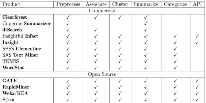
Product Preprocess Associate Cluster Summarize Categorize API Commercial Clearforest X X X X CopernicSummarizer X X dtSearch X X X InsightfulInfact X X X X X X Inxight X X X X X X SPSSClementine X X X X X
SASText Miner X X X X X
TEMIS X X X X X WordStat X X X X X Open Source GATE X X X X X X RapidMiner X X X X X X Weka/KEA X X X X X X R/tm X X X X X X
Table 1: Overview of text mining products and available features. A feature is marked as implemented (denoted asX) if the official feature description of each product explicitly lists it.
Cluster: clustering of similar documents into the same groups,
Summarize: summarization of important concepts in a text. Typically these are high-frequency terms,
Categorize: classification of texts into predefined categories, and
API: availability of application programming interfaces to extend the program with plug-ins. Table1 gives an overview over the most-used commercial text mining products ( Piatetsky-Shapiro 2005), selected open source text mining tool kits, and features. Commercial prod-ucts includeClearforest, a text-driven business intelligence solution, CopernicSummarizer, a summarizing software extracting key concepts and relevant sentences,dtSearch, a document search tool, InsightfulInfact, a search and analysis text mining tool, Inxight, an integrated suite of tools for search, extraction, and analysis of text,SPSS Clementine, a data and text mining workbench,SAS Text Miner, a suite of tools for knowledge discovery and knowledge extraction in texts, TEMIS, a tool set for text extraction, text clustering, and text catego-rization, andWordStat, a product for computer assisted text analysis.
From Table1we see that most commercial tools lack easy-to-use API integration and provide a relatively monolithic structure regarding extensibility since their source code is not freely available.
Among well known open source data mining tools offering text mining functionality is the Weka (Witten and Frank 2005) suite, a collection of machine learning algorithms for data mining tasks also offering classification and clustering techniques with extension projects for text mining, like KEA (Witten et al. 2005) for keyword extraction. It provides good API support and has a wide user base. Then there is GATE (Cunningham et al. 2002),
an established text mining framework with architecture for language processing, information extraction, ontology management and machine learning algorithms. It is fully written in
Java. Another tools are RapidMiner (formerly Yale (Mierswa et al. 2006)), a system for knowledge discovery and data mining, and Pimiento (Adeva and Calvo 2006), a basic Java
framework for text mining. However, many existing open-source products tend to offer rather specialized solutions in the text mining context, such as Shogun (Sonnenburg et al. 2006), a toolbox for string kernels, or the Bow toolkit (McCallum 1996), a C library useful for statistical text analysis, language modeling and information retrieval. In R the extension packagettda (Mueller 2006) provides some methods for textual data analysis.
We present a text mining framework for the open source statistical computing environmentR
centered around the new extension packagetm (Feinerer 2007b). This open source package, with a focus on extensibility based on generic functions and object-oriented inheritance, pro-vides the basic infrastructure necessary to organize, transform, and analyze textual data. R
has proven over the years to be one of the most versatile statistical computing environments available, and offers a battery of both standard and state-of-the-art methodology. However, the scope of these methods was often limited to “classical”, structured input data formats (such as data frames in R). The tm package provides a framework that allows researchers and practitioners to apply a multitude of existing methods to text data structures as well. In addition, advanced text mining methods beyond the scope of most today’s commercial products, like string kernels or latent semantic analysis, can be made available via exten-sion packages, such as kernlab (Karatzoglou et al. 2004, 2006) or lsa (Wild 2005), or via interfaces to established open source toolkits from the data/text mining field like Weka or OpenNLP (Bierner et al. 2007) from the natural languange processing community. So tm provides a framework for flexible integration of premier statistical methods fromR, interfaces to well known open source text mining infrastructure and methods, and has a sophisticated modularized extension mechanism for text mining purposes.
This paper is organized as follows. Section2elaborates, on a conceptual level, important ideas and tasks a text mining framework should be able to deal with. Section3 presents the main structure of our framework, its algorithms, and ways to extend the text mining framework for custom demands. Section4describes preprocessing mechanisms, like data import, stemming, stopword removal and synonym detection. Section 5 shows how to conduct typical text mining tasks within our framework, like count-based evaluation methods, text clustering with term-document matrices, text classification, and text clustering with string kernels. Section6 presents an application oftmby analyzing theR-devel 2006 mailing list. Section7concludes. Finally AppendixA gives a very detailed and technical description oftmdata structures.
2. Conceptual process and framework
A text mining analysis involves several challenging process steps mainly influenced by the fact that texts, from a computer perspective, are rather unstructured collections of words. A text mining analyst typically starts with a set of highly heterogeneous input texts. So the first step is to import these texts into one’s favorite computing environment, in our case
R. Simultaneously it is important to organize and structure the texts to be able to access them in a uniform manner. Once the texts are organized in a repository, the second step is tidying up the texts, including preprocessing the texts to obtain a convenient representa-tion for later analysis. This step might involve text reformatting (e.g., whitespace removal),
stopword removal, or stemming procedures. Third, the analyst must be able to transform the preprocessed texts into structured formats to be actually computed with. For “classical” text mining tasks, this normally implies the creation of a so-called term-document matrix, probably the most common format to represent texts for computation. Now the analyst can work and compute on texts with standard techniques from statistics and data mining, like clustering or classification methods.
This rather typical process model highlights important steps that call for support by a text mining infrastructure: A text mining framework must offer functionality for managing text documents, should abstract the process of document manipulation and ease the usage of heterogeneous text formats. Thus there is a need for a conceptual entity similar to a database holding and managing text documents in a generic way: we call this entity atext document collection orcorpus.
Since text documents are present in different file formats and in different locations, like a com-pressed file on the Internet or a locally stored text file with additional annotations, there has to be an encapsulating mechanism providing standardized interfaces to access the document data. We subsume this functionality in so-calledsources.
Besides the actual textual data many modern file formats provide features to annotate text documents (e.g., XML with special tags), i.e., there is metadata available which further de-scribes and enriches the textual content and might offer valuable insights into the document structure or additional concepts. Also, additional metadata is likely to be created during an analysis. Therefore the framework must be able to alleviate metadata usage in a convenient way, both on a document level (e.g., short summaries or descriptions of selected documents) and on a collection level (e.g., collection-wide classification tags).
Alongside the data infrastructure for text documents the framework must provide tools and algorithms to efficiently work with the documents. That means the framework has to have functionality to perform common tasks, like whitespace removal, stemming or stopword dele-tion. We denote such functions operating on text document collections as transformations. Another important concept isfiltering which basically involves applying predicate functions on collections to extract patterns of interest. A surprisingly challenging operation is the one of joining text document collections. Merging sets of documents is straightforward, but merging metadata intelligently needs a more sophisticated handling, since storing metadata from dif-ferent sources in successive steps necessarily results in a hierarchical, tree-like structure. The challenge is to keep these joins and subsequent look-up operations efficient for large document collections.
Realistic scenarios in text mining use at least several hundred text documents ranging up to several hundred thousands of documents. This means a compact storage of the documents in a document collection is relevant for appropriate RAM usage — a simple approach would hold all documents in memory once read in and bring down even fully RAM equipped systems shortly with document collections of several thousands text documents. However, simple database orientated mechanisms can already circumvent this situation, e.g., by holding only pointers or hashtables in memory instead of full documents.
Text mining typically involves doing computations on texts to gain interesting information. The most common approach is to create a so-calledterm-document matrix holding frequences of distinct terms for each document. Another approach is to compute directly on character sequences as is done by string kernel methods. Thus the framework must allow export
mech-Application Layer Text Mining Framework
RSystem Environment
lsa tm
wordnetRWeka openNLPkernlab Rstem Snowball
XML
R
Figure 1: Conceptual layers and packages.
anisms for term-document matrices and provide interfaces to access the document corpora as plain character sequences.
Basically, the framework and infrastructure supplied by tm aims at implementing the con-ceptual framework presented above. The next section will introduce the data structures and algorithms provided.
3. Data structures and algorithms
In this section we explain both the data structures underlying our text mining framework and the algorithmic background for working with these data structures. We motivate the general structure and show how to extend the framework for custom purposes.
Commercial text mining products (Daviet al.2005) are typically built in monolithic structures regarding extensibility. This is inherent as their source code is normally not available. Also, quite often interfaces are not disclosed and open standards hardly supported. The result is that the set of predefined operations is limited, and it is hard (or expensive) to write plug-ins. Therefore we decided to tackle this problem by implementing a framework for accessing text data structures in R. We concentrated on a middle ware consisting of several text mining classes that provide access to various texts. On top of this basic layer we have a virtual application layer, where methods operate without explicitly knowing the details of internal text data structures. The text mining classes are written as abstract and generic as possible, so it is easy to add new methods on the application layer level. The framework uses the
S4 (Chambers 1998) class system to capture an object oriented design. This design seems best capable of encapsulating several classes with internal data structures and offers typed methods to the application layer.
This modular structure enablestmto integrate existing functionality from other text mining tool kits. E.g., we interface with theWekaand OpenNLPtool kits, viaRWeka(Horniket al. 2007)—and Snowball (Hornik 2007b) for its stemmers—and openNLP (Feinerer 2007a), re-spectively. In detail Weka gives us stemming and tokenization methods, whereas OpenNLP offers amongst others tokenization, sentence detection, and part of speech tagging (Bill 1995). We can plug in this functionality at various points intm’s infrastructure, e.g., for preprocess-ing via transformation methods (see Section 4), for generating term-document matrices (see Paragraph 3.1.4), or for custom functions when extending tm’s methods (see Section3.3). Figure1 shows both the conceptual layers of our text mining infrastructure and typical pack-ages arranged in them. The system environment is made up of theRcore and theXML( Tem-ple Lang 2006) package for handling XML documents internally, the text mining framework consists of our new tmpackage with some help ofRstem(Temple Lang 2004) orSnowballfor
TermDocMatrix Weighting : String Data : Matrix Corpus DMetaData : DataFrame DBControl : List XMLTextDocument URI : Call Cached : Boolean PlainTextDocument URI : Call Cached : Boolean character XMLDocument TextRepository RepoMetaData : List TextDocument Author : String DateTimeStamp : Date Description : String ID : String Origin : String Heading : String LocalMetaData : List Language : String 1..* 1 MetaDataNode NodeID : Integer MetaData : List Children : List NewsgroupDocument URI : Call Cached : Boolean Newsgroup : String 1 1..* StructuredTextDocument URI : Call Cached : Boolean 1 CMetaData 1
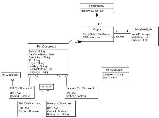
Figure 2: UML class diagram of thetm package.
stemming, whereas some packages provide both infrastructure and applications, like word-net(Feinerer 2007c),kernlabwith its string kernels, or theRWekaandopenNLPinterfaces. A typical application might belsawhich can use our middleware: the key data structure for la-tent semantic analysis (LSALandaueret al.1998;Deerwesteret al.1990) is a term-document matrix which can be easily exported from ourtmframework. As defaultlsaprovides its own (rather simple) routines for generating term-document matrices, so one can either use lsa natively or enhance it with tm for handling complex input formats, preprocessing, and text manipulations, e.g., as used byFeinerer and Wild(2007).
3.1. Data structures
We start by explaining the data structures: The basic framework classes and their interac-tions are depicted in Figure 2 as a UML class diagram (Fowler 2003) with implementation independent UML datatypes. In this section we give an overview how the classes interoperate and work whereas an in-depth description is found in the AppendixA to be used as detailed reference.
Text document collections
also denoted as corpus in linguistics (Corpus). It represents a collection of text documents and can be interpreted as a database for texts. Its elements are TextDocuments holding the actual text corpora and local metadata. The text document collection has two slots for storing global metadata and one slot for database support.
We can distinguish two types of metadata, namelyDocument Metadata and Collection Meta-data. Document metadata (DMetaData) is for information specific to text documents but with an own entity, like classification results (it holds both the classifications for each docu-ments but in addition global information like the number of classification levels). Collection metadata (CMetaData) is for global metadata on the collection level not necessarily related to single text documents, like the creation date of the collection (which is independent from the documents within the collection).
The database slot (DBControl) controls whether the collection uses a database backend for storing its information, i.e., the documents and the metadata. If activated, packagetm tries to hold as few bits in memory as possible. The main advantage is to be able to work with very large text collections, a shortcoming might be slower access performance (since we need to load information from the disk on demand). Also note that activated database support introduces persistent object semantics since changes are written to the disk which other objects (pointers) might be using.
Objects of classCorpus can be manually created by
R> new("Corpus", .Data = ..., DMetaData = ..., CMetaData = ...,
+ DBControl = ...)
where .Data has to be the list of text documents, and the other arguments have to be the document metadata, collection metadata and database control parameters. Typically, however, we use the Corpus constructor to generate the right parameters given following arguments:
object : a Sourceobject which abstracts the input location.
readerControl : a list with the three components reader, language, and load, giving a reader capable of reading in elements delivered from the document source, a string giving the ISO language code (typically in ISO 639 or ISO 3166 format, e.g., en_US for American English), and a Boolean flag indicating whether the user wants to load documents immediately into memory or only when actually accessed (we denote this feature asload on demand).
The tmpackage ships with several readers (use getReaders()to list available readers) described in Table 2.
dbControl : a list with the three componentsuseDb,dbName and dbTypesetting the respec-tive DBControlvalues (whether database support should be activated, the file name to the database, and the database type).
An example of a constructor call might be R> Corpus(object = ...,
Reader Description
readPlain() Read in files as plain text ignoring metadata
readRCV1() Read in files in Reuters Corpus Volume 1 XML format readReut21578XML() Read in files in Reuters-21578 XML format
readGmane() Read in Gmane RSS feeds
readNewsgroup() Read in newsgroup posting (e-mails) in UCI KDD archive format readPDF() Read in PDF documents
readDOC() Read in MS Word documents
readHTML() Read in simply structured HTML documents Table 2: Available readers in the tmpackage.
+ language = "en_US",
+ load = FALSE),
+ dbControl = list(useDb = TRUE,
+ dbName = "texts.db",
+ dbType = "DB1"))
whereobject denotes a valid instance of class Source. We will cover sources in more detail later.
Text documents
The next core class is a text document (TextDocument), the basic unit managed by a text document collection. It is an abstract class, i.e., we must derive specific document classes to obtain document types we actually use in daily text mining. Basic slots areAuthor holding the text creators, DateTimeStamp for the creation date, Description for short explanations or comments,IDfor a unique identification string,Origindenoting the document source (like the news agency or publisher),Heading for the document title, Language for the document language, andLocalMetaData for any additional metadata.
The main rationale is to extend this class as needed for specific purposes. This offers great flexibility as we can handle any input format internally but provide a generic interface to other classes. The following four classes are derived classes implementing documents for common file formats and come with the package: XMLTextDocument for XML documents, PlainTextDocument for simple texts, NewsgroupDocument for newsgroup postings and e-mails, and StructuredTextDocument for more structured documents (e.g., with explicitly marked paragraphs, etc.).
Text documents can be created manually, e.g., via
R> new("PlainTextDocument", .Data = "Some text.", URI = uri, Cached = TRUE, + Author = "Mr. Nobody", DateTimeStamp = Sys.time(),
+ Description = "Example", ID = "ID1", Origin = "Custom", + Heading = "Ex. 1", Language = "en_US")
setting all arguments for initializing the class (uri is a shortcut for a reference to the input, e.g., a call to a file on disk). In most cases text documents are returned by reader functions, so there is no need for manual construction.
Text repositories
The next class from our framework is a so-called text repository which can be used to keep track of text document collections. The classTextRepository is conceptualized for storing representations of the same text document collection. This allows to backtrack transfor-mations on text documents and access the original input data if desired or necessary. The dynamic slotRepoMetaData can help to save the history of a text document collection, e.g., all transformations with a time stamp in form of tag-value pair metadata.
We construct a text repository by calling R> new("TextRepository",
+ .Data = list(Col1, Col2), RepoMetaData = list(created = "now")) whereCol1 andCol2 are text document collections.
Term-document matrices
Finally we have a class for term-document matrices (Berry 2003;Shawe-Taylor and Cristianini 2004), probably the most common way of representing texts for further computation. It can be exported from aCorpus and is used as a bag-of-words mechanism which means that the order of tokens is irrelevant. This approach results in a matrix with document IDs as rows and terms as columns. The matrix elements are term frequencies.
For example, consider the two documents withIDs 1 and 2 and their contentstext mining is funanda text is a sequence of words, respectively. Then the term-document matrix is
a fun is mining of sequence text words
1 0 1 1 1 0 0 1 0
2 2 0 1 0 1 1 1 1
TermDocMatrix provides such a term-document matrix for a given Corpus element. It has the slotData of the formal class Matrix from packageMatrix (Bates and Maechler 2007) to hold the frequencies in compressed sparse matrix format.
Instead of using the term frequency (weightTf) directly, one can use different weightings. The slotWeighting of a TermDocMatrix provides this facility by calling a weighting function on the matrix elements. Available weighting schemes include thebinary frequency (weightBin) method which eliminates multiple entries, or the inverse document frequency (weightTfIdf) weighting giving more importance to discriminative compared to irrelevant terms. Users can apply their own weighting schemes by passing over custom weighting functions toWeighting. Again, we can manually construct a term-document matrix, e.g., via
R> new("TermDocMatrix", Data = tdm, Weighting = weightTf) where tdmdenotes a sparseMatrix.
Typically, we will use the TermDocMatrix constructor instead for creating a term-document matrix from a text document collection. The constructor provides a sophisticated modular structure for generating such a matrix from documents: you can plug in modules for each processing step specified via a control argument. E.g., we could use an n-gram tokenizer (NGramTokenizer) from the Weka toolkit (via RWeka) to tokenize into phrases instead of single words
Source getElem() : Element stepNext() : void eoi() : Boolean LoDSupport : Boolean Position : Integer DefaultReader : function Encoding : String DirSource FileList : String Load : Boolean CSVSource URI : Call Content : String ReutersSource URI : Call Content : XMLDocument GmaneSource URI : Call Content : XMLDocument
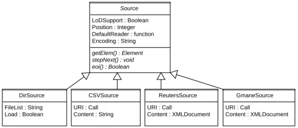
Figure 3: UML class diagram for Sources.
R> TermDocMatrix(col, control = list(tokenize = NGramTokenizer)) or a tokenizer from theOpenNLP toolkit (viaopenNLP’stokenizefunction) R> TermDocMatrix(col, control = list(tokenize = tokenize))
wherecoldenotes a text collection. Instead of using a classical tokenizer we could be inter-ested in phrases or whole sentences, so we take advantage of the sentence detection algorithms offered byopenNLP.
R> TermDocMatrix(col, control = list(tokenize = sentDetect))
Similarly, we can use external modules for all other processing steps (mainly via internal calls totermFreq which generates a term frequency vector from a text document and gives an extensive list of available control options), like stemming (e.g., the Weka stemmers via theSnowball package), stopword removal (e.g., via custom stopword lists), or user supplied dictionaries (a method to restrict the generated terms in the term-document matrix). This modularization allows synergy gains between available established toolkits (likeWekaor OpenNLP) and allowstm to utilize available functionality.
Sources
The tm package uses the concept of a so-calledsource to encapsulate and abstract the doc-ument input process. This allows to work with standardized interfaces within the package without knowing the internal structures of input document formats. It is easy to add support for new file formats by inheriting from theSource base class and implementing the interface methods.
Figure 3 shows a UML diagram with implementation independent UML data types for the Sourcebase class and existing inherited classes.
A source is aVIRTUAL class (i.e., it cannot be instantiated, only classes may be derived from it) and abstracts the input location and serves as the base class for creating inherited classes for specialized file formats. It has four slots, namelyLoDSupportindicating load on demand
support,Position holding status information for internal navigation, DefaultReader for a default reader function, andEncodingfor the encoding to be used by internalRroutines for accessing texts via the source (defaults to UTF-8 for all sources).
The following classes are specific source implementations for common purposes:DirSourcefor directories with text documents,CSVSourcefor documents stored in CSV files,ReutersSource for special Reuters file formats, and GmaneSource for so-called RSS feeds as delivered by Gmane (Ingebrigtsen 2007).
A directory source can manually be created by calling
R> new("DirSource", LoDSupport = TRUE, FileList = dir(), Position = 0, + DefaultReader = readPlain, Encoding = "latin1")
where readPlain() is a predefined reader function in tm. Again, we provide wrapper func-tions for the various sources.
3.2. Algorithms
Next, we present the algorithmic side of our framework. We start with the creation of a text document collection holding some plain texts in Latin language from Ovid’sars amato-ria (Naso 2007). Since the documents reside in a separate directory we use the DirSource and ask for immediate loading into memory. The elements in the collection are of class PlainTextDocument since we use the default reader which reads in the documents as plain text:
R> txt <- system.file("texts", "txt", package = "tm") R> (ovid <- Corpus(DirSource(txt),
+ readerControl = list(reader = readPlain,
+ language = "la",
+ load = TRUE)))
A text document collection with 5 text documents
Alternatively we could activate database support such that only relevant information is kept in memory:
R> Corpus(DirSource(txt),
+ readerControl = list(reader = readPlain,
+ language = "la", load = TRUE),
+ dbControl = list(useDb = TRUE,
+ dbName = "/home/user/oviddb",
+ dbType = "DB1"))
The loading and unloading of text documents and metadata of the text document collection is transparent to the user, i.e., fully automatic. Manipulations affecting R text document collections are written out to the database, i.e., we obtain persistent object semantics in contrast to R’s common semantics.
We have implemented both accessor and set functions for the slots in our classes such that slot information can easily be accessed and modified, e.g.,
R> ID(ovid[[1]]) [1] "1"
gives theIDslot attribute of the first ovid document. With e.g., R> Author(ovid[[1]]) <- "Publius Ovidius Naso"
we modify the Author slot information.
To see all available metadata for a text document, use meta(), e.g., R> meta(ovid[[1]])
Available meta data pairs are:
Author : Publius Ovidius Naso Cached : TRUE DateTimeStamp: 2008-03-16 14:49:58 Description : ID : 1 Heading : Language : la Origin :
URI : file /home/feinerer/lib/R/library/tm/texts/txt/ovid_1.txt UTF-8
Dynamic local meta data pairs are: list()
Further we have implemented following operators and functions for text document collections: [ The subset operator allows to specify a range of text documents and automatically en-sures that a valid text collection is returned. Further the DMetaData data frame is automatically subsetted to the specific range of documents.
R> ovid[1:3]
A text document collection with 3 text documents
[[ accesses a single text document in the collection. A specialshow() method for plain text documents pretty prints the output.
R> ovid[[1]]
[1] " Si quis in hoc artem populo non novit amandi," [2] " hoc legat et lecto carmine doctus amet." [3] " arte citae veloque rates remoque moventur," [4] " arte leves currus: arte regendus amor." [5] ""
[7] " Tiphys in Haemonia puppe magister erat:" [8] " me Venus artificem tenero praefecit Amori;" [9] " Tiphys et Automedon dicar Amoris ego."
[10] " ille quidem ferus est et qui mihi saepe repugnet:" [11] ""
[12] " sed puer est, aetas mollis et apta regi." [13] " Phillyrides puerum cithara perfecit Achillem," [14] " atque animos placida contudit arte feros." [15] " qui totiens socios, totiens exterruit hostes," [16] " creditur annosum pertimuisse senem." c() Concatenates several text collections to a single one.
R> c(ovid[1:2], ovid[3:4])
A text document collection with 4 text documents
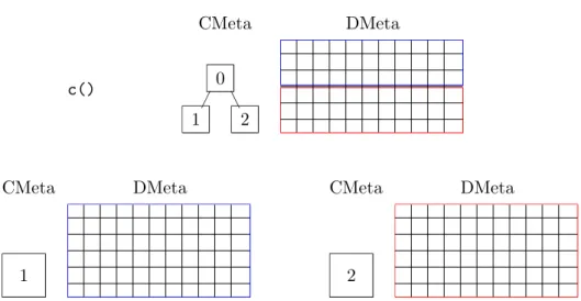
The metadata of both text document collections is merged, i.e., a new root node is created in the CMetaData tree holding the concatenated collections as children, and the DMetaData data frames are merged. Column names existing in one frame but not the other are filled up with NA values. The whole process of joining the metadata is depicted in Figure 4. Note that concatenation of text document collections with activated database backends is not supported since it might involve the generation of a new database (as a collection has to have exactly one database) and massive copying of database values.
length() Returns the number of text documents in the collection. R> length(ovid) [1] 5 c() CMeta DMeta 1 CMeta DMeta 2 CMeta DMeta 0 2 1 A
show() A custom print method. Instead of printing all text documents (consider a text collection could consist of several thousand documents, similar to a database), only a short summarizing message is printed.
summary() A more detailed message, summarizing the text document collection. Available metadata is listed.
R> summary(ovid)
A text document collection with 5 text documents
The metadata consists of 2 tag-value pairs and a data frame Available tags are:
create_date creator
Available variables in the data frame are: MetaID
inspect() This function allows to actually see the structure which is hidden byshow() and summary() methods. Thus all documents and metadata are printed, e.g.,
inspect(ovid).
tmUpdate() takes as argument a text document collection, a source with load on demand support and areaderControlas found in theCorpusconstructor. The source is checked for new files which do not already exist in the document collection. Identified new files are parsed and added to the existing document collection, i.e., the collection is updated, and loaded into memory if demanded.
R> tmUpdate(ovid, DirSource(txt))
A text document collection with 5 text documents
Text documents and metadata can be added to text document collections withappendElem() and appendMeta(), respectively. As already described earlier the text document collection has two types of metadata: one is the metadata on the document collection level (cmeta), the other is the metadata related to the individual documents (e.g., clusterings) (dmeta) with an own entity in form of a data frame.
R> ovid <- appendMeta(ovid,
+ cmeta = list(test = c(1,2,3)),
+ dmeta = list(clust = c(1,1,2,2,2)))
R> summary(ovid)
A text document collection with 5 text documents
The metadata consists of 3 tag-value pairs and a data frame Available tags are:
create_date creator test
Available variables in the data frame are: MetaID clust
R> CMetaData(ovid)
An object of class "MetaDataNode" Slot "NodeID": [1] 0 Slot "MetaData": $create_date [1] "2008-03-16 14:49:58 CET" $creator LOGNAME "feinerer" $test [1] 1 2 3 Slot "children": list() R> DMetaData(ovid) MetaID clust 1 0 1 2 0 1 3 0 2 4 0 2 5 0 2
For the method appendElem(), which adds the data object of class TextDocument to the data segment of the text document collectionovid, it is possible to give a column of values in the data frame for the added data element.
R> (ovid <- appendElem(ovid, data = ovid[[1]], list(clust = 1))) A text document collection with 6 text documents
The methodsappendElem(),appendMeta()and removeMeta()also exist for the class TextRepository, which is typically constructed by passing a initial text document collection, e.g.,
R> (repo <- TextRepository(ovid))
The argument syntax for adding data and metadata is identical to the arguments used for text collections (since the functions are generic) but now we add data (i.e., in this case whole text document collections) and metadata to a text repository. Since text repositories’ meta-data only may contain repository specific metameta-data, the argumentdmetaofappendMeta()is ignored andcmeta must be used to pass over repository metadata.
R> repo <- appendElem(repo, ovid, list(modified = date())) R> repo <- appendMeta(repo, list(moremeta = 5:10))
R> summary(repo)
A text repository with 2 text document collections The repository metadata consists of 3 tag-value pairs Available tags are:
created modified moremeta R> RepoMetaData(repo) $created [1] "2008-03-16 14:49:58 CET" $modified [1] "Sun Mar 16 14:49:58 2008" $moremeta [1] 5 6 7 8 9 10
The methodremoveMeta()is implemented both for text document collections and text repos-itories. In the first case it can be used to delete metadata from theCMetaDataandDMetaData slots, in the second case it removes metadata fromRepoMetaData. The function has the same signature asappendMeta().
In addition there is the methodmeta()as a simplified uniform mechanism to access metadata. It provides accessor and set methods for text collections, text repositories and text documents (as already shown for a document from the ovid corpus at the beginning of this section). Especially for text collections it is a simplification since it provides a uniform way to edit DMetaDataand CMetaData (typecorpus), e.g.,
R> meta(ovid, type = "corpus", "foo") <- "bar" R> meta(ovid, type = "corpus")
An object of class "MetaDataNode" Slot "NodeID":
[1] 0
Slot "MetaData": $create_date
[1] "2008-03-16 14:49:58 CET" $creator LOGNAME "feinerer" $test [1] 1 2 3 $foo [1] "bar" Slot "children": list() R> meta(ovid, "someTag") <- 6:11 R> meta(ovid)
MetaID clust someTag
1 0 1 6 2 0 1 7 3 0 2 8 4 0 2 9 5 0 2 10 6 0 1 11
In addition we provide a generic interface to operate on text document collections, i.e., trans-form and filter operations. This is of great importance in order to provide a high-level concept for often used operations on text document collections. The abstraction avoids the user to take care of internal representations but offers clearly defined, implementation independent, operations.
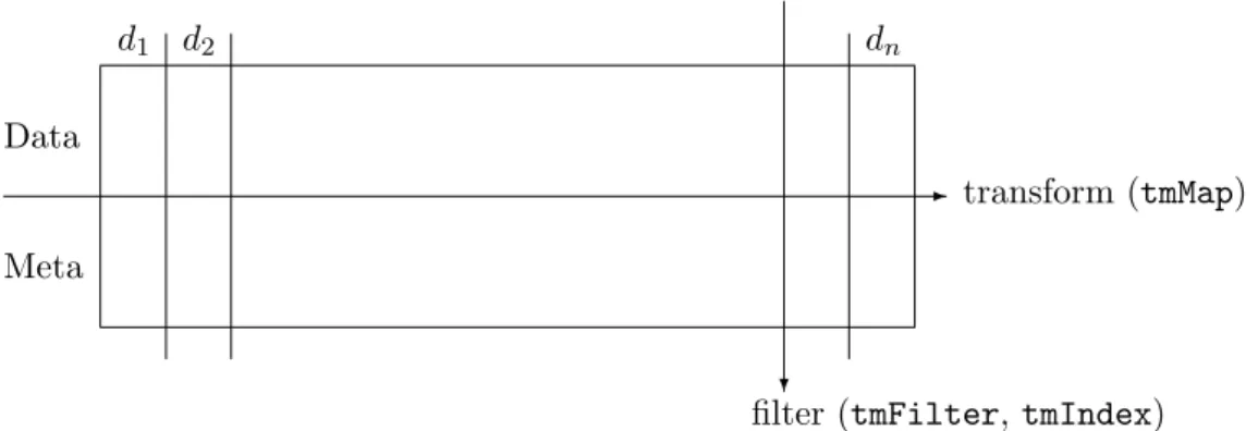
Transformations operate on each text document in a text document collection by applying a function to them. Thus we obtain another representation of the whole text document collec-tion. Filter operations instead allow to identify subsets of the text document collection. Such a subset is defined by a function applied to each text document resulting in a Boolean answer. Hence formally the filter function is just a predicate function. This way we can easily identify documents with common characteristics. Figure 5 visualizes this process of transformations and filters. It shows a text document collection with text documents d1, d2, . . . , dn consisting
of corpus data (Data) and the document specific metadata data frame (Meta).
Transformations are done via the tmMap() function which applies a function FUN to all el-ements of the collection. Basically, all transformations work on single text documents and tmMap()just applies them to all documents in a document collection. E.g.,
R> tmMap(ovid, FUN = tmTolower)
d1 d2 dn
?
filter (tmFilter,tmIndex) Data
Meta
transform (tmMap)
-Figure 5: Generic transform and filter operations on a text document collection. Transformation Description
asPlain() Converts the document to a plain text document loadDoc() Triggers load on demand
removeCitation() Removes citations from e-mails
removeMultipart() Removes non-text from multipart e-mails removeNumbers() Removes numbers
removePunctuation() Removes punctuation marks removeSignature() Removes signatures from e-mails removeWords() Removes stopwords
replaceWords() Replaces a set of words with a given phrase stemDoc() Stems the text document
stripWhitespace() Removes extra whitespace tmTolower() Conversion to lower case letters
Table 3: Transformations shipped withtm.
appliestmTolower() to each text document in the ovid collection and returns the modified collection. Optional parameters... are passed directly to the functionFUNif given totmMap() allowing detailed arguments for more complex transformations. Further the document specific metadata data frame is passed to the function as argument DMetaData to enable transfor-mations based on information gained by metadata investigation. Table 3 gives an overview over available transformations (usegetTransformations()to list available transformations) shipped with tm.
Filters (use getFilters() to list available filters) are performed via the tmIndex() and tmFilter()functions. Both function have the same internal behavior except thattmIndex() returns Boolean values whereastmFilter() returns the corresponding documents in a new Corpus. Both functions take as input a text document collection, a function FUN, a flag doclevelindicating whether FUN is applied to the collection itself (default) or to each doc-ument separately, and optional parameters ... to be passed to FUN. As in the case with transformations the document specific metadata data frame is passed to FUN as argument DMetaData. E.g., there is a full text search filtersearchFullText() available which accepts regular expressions and is applied on the document level:
A text document collection with 2 text documents
Any valid predicate function can be used as custom filter function but for most cases the default filter sFilter() does its job: it integrates a minimal query language to filter meta-data. Statements in this query language are statements as used for subsetting data frames, i.e, a statement s is of format "tag1 == ’expr1’ & tag2 == ’expr2’ & ...". Tags in s represent data frame metadata variables. Variables only available at the document level are shifted up to the data frame if necessary. Note that the metadata tags for the slotsAuthor, DateTimeStamp, Description, ID, Origin, Language and Heading of a text document are author, datetimestamp, description, identifier, origin, language and heading, re-spectively, to avoid name conflicts. For example, the following statement filters out those documents having anIDequal to 2:
R> tmIndex(ovid, "identifier == '2'") [1] FALSE TRUE FALSE FALSE FALSE FALSE
As you see the query is applied to the metadata data frame (the document localIDmetadata is shifted up to the metadata data frame automatically since it appears in the statement) thus an investigation on document level is not necessary.
3.3. Extensions
The presented framework classes already build the foundation for typical text mining tasks but we emphasize available extensibility mechanisms. This allows the user to customize classes for specific demands. In the following, we sketch an example (only showing the main elements and function signatures).
Suppose we want to work with an RSS newsgroup feed as delivered by Gmane (Ingebrigtsen 2007) and analyze it in R. Since we already have a class for handling newsgroup mails as found in the Newsgroup data set from the UCI KDD archive (Hettich and Bay 1999) we will reuse it as it provides everything we need for this example. At first, we derive a new source class for our RSS feeds:
R> setClass("GmaneSource",
+ representation(URI = "ANY", Content = "list"), + contains = c("Source"))
which inherits from the Source class and provides slots as for the existing ReutersSource class, i.e.,URIfor holding a reference to the input (e.g., a call to a file on disk) and Content to hold the XML tree of the RSS feed.
Next we can set up the constructor for the classGmaneSource: R> setMethod("GmaneSource",
+ signature(object = "ANY"),
+ function(object, encoding = "UTF-8") {
+ ## ---code
chunk---+ new("GmaneSource", LoDSupport = FALSE, URI = object,
+ Content = content, Position = 0, Encoding = encoding)
where--code chunk--is a symbolic anonymous shorthand for reading in the RSS file, parsing it, e.g., with methods provided in theXMLpackage, and filling the contentvariable with it. Next we need to implement the three interface methods a source must provide:
R> setMethod("stepNext", + signature(object = "GmaneSource"), + function(object) { + object@Position <- object@Position + 1 + object + })
simply updates the position counter for using the next item in the XML tree, R> setMethod("getElem",
+ signature(object = "GmaneSource"),
+ function(object) {
+ ## ---code
chunk---+ list(content = content, uri = object@URI)
+ })
returns a list with the element’s content at the active position (which is extracted in--code chunk--) and the corresponding unique resource identifier, and
R> setMethod("eoi",
+ signature(object = "GmaneSource"),
+ function(object) {
+ length(object@Content) <= object@Position
+ })
indicates the end of the XML tree.
Finally we write a custom reader function which extracts the relevant information out of RSS feeds:
R> readGmane <- FunctionGenerator(function(...) { + function(elem, load, language, id) {
+ ## ---code
chunk---+ new("NewsgroupDocument", .Data = content, URI = elem$uri,
+ Cached = TRUE, Author = author, DateTimeStamp = datetimestamp, + Description = "", ID = id, Origin = origin, Heading = heading,
+ Language = language, Newsgroup = newsgroup)
+ }
+ })
The function shows how a customFunctionGeneratorcan be implemented which returns the reader as return value. The reader itself extracts relevant information via XPath expressions in the function body’s--code chunk--and returns a NewsgroupDocument as desired. The full implementation comes with the tm package such that we can use the source and reader to access Gmane RSS feeds:
R> rss <- system.file("texts", "gmane.comp.lang.r.gr.rdf", package = "tm") R> Corpus(GmaneSource(rss), readerControl = list(reader = readGmane,
+ language = "en_US", load = TRUE))
A text document collection with 21 text documents
Since we now have a grasp about necessary steps to extend the framework we want to show how easy it is to produce realistic readers by giving an actual implementation for a highly desired feature in theRcommunity: a PDF reader. The reader expects the two command line toolspdftotext and pdfinfoinstalled to work properly (both programs are freely available for common operating systems, e.g., via thepopplerorxpdf tool suites).
R> readPDF <- FunctionGenerator(function(...) { + function(elem, load, language, id) {
+ ## get metadata
+ meta <- system(paste("pdfinfo", as.character(elem$uri[2])),
+ intern = TRUE)
+
+ ## extract and store main information, e.g.: + heading <- gsub("Title:[[:space:]]*", "",
+ grep("Title:", meta, value = TRUE))
+
+ ## [... similar for other metadata ...] +
+ ## extract text from PDF using the external pdftotext utility:
+ corpus <- paste(system(paste("pdftotext", as.character(elem$uri[2]), "-"),
+ intern = TRUE),
+ sep = "\n", collapse = "") +
+ ## create new text document object:
+ new("PlainTextDocument", .Data = corpus, URI = elem$uri, Cached = TRUE, + Author = author, DateTimeStamp = datetimestamp,
+ Description = description, ID = id, Origin = origin, + Heading = heading, Language = language)
+ }
+ })
Basically we usepdfinfoto extract the metadata, search the relevant tags for filling metadata slots, and usepdftotext for acquiring the text corpus.
We have seen extensions for classes, sources and readers. But we can also write custom transformation and filter functions. E.g., a custom generic transform function could look like R> setGeneric("myTransform", function(object, ...) standardGeneric("myTransform")) R> setMethod("myTransform", signature(object = "PlainTextDocument"),
+ function(object, ..., DMetaData) {
+ Content(object) <- doSomeThing(object, DMetaData)
+ return(object)
where we change the text corpus (i.e., the actual text) based on doSomeThing’s result and return the document again. In case of a filter function we would return a Boolean value. Summarizing, this section showed that own fully functional classes, sources, readers, trans-formations and filters can be contributed simply by giving implementations for interface def-initions.
Based on the presented framework and its algorithms the following sections will show how to use tmto ease text mining tasks in R.
4. Preprocessing
Input texts in their native raw format can be an issue when analyzing these with text mining methods since they might contain many unimportant stopwords (like andorthe) or might be formatted inconveniently. Therefore preprocessing, i.e., applying methods for cleaning up and structuring the input text for further analysis, is a core component in practical text mining studies. In this section we will discuss how to perform typical preprocessing steps in the tm package.
4.1. Data import
One very popular data set in text mining research is the Reuters-21578 data set (Lewis 1997). It now contains over 20000 stories (the original version contained 21578 documents) from the Reuters news agency with metadata on topics, authors and locations. It was compiled by David Lewis in 1987, is publicly available and is still one of the most widely used data sets in recent text mining articles (see, e.g., Lodhiet al. 2002).
The original Reuters-21578 XML data set consists of a set of XML files with about 1000 articles per XML file. In order to enable load on demand the method preprocessReut21578XML() can be used to split the articles into separate files such that each article is stored in its own XML file. Reuters examples in the tmpackage and Reuters data sets used in this paper have already been preprocessed with this function.
Documents in the Reuters XML format can easily be read in with existing parsing functions R> reut21578XMLgz <- system.file("texts", "reut21578.xml.gz", package = "tm") R> (Reuters <- Corpus(ReutersSource(gzfile(reut21578XMLgz)),
+ readerControl = list(reader = readReut21578XML,
+ language = "en_US",
+ load = TRUE)))
A text document collection with 10 text documents
Note that connections can be passed over to ReutersSource, e.g., we can compress our files on disk to save space without losing functionality. The package further supports Reuters Corpus Volume 1 (Lewis et al. 2004)—the successor of the Reuters-21578 data set—which can be similarly accessed via predefined readers (readRCV1()).
The default encoding used by sources is always assumed to be UTF-8. Anyway, one can man-ually set the encoding via the encodingparameter (e.g.,DirSource("texts/", encoding =
"latin1")) or by creating a connection with an alternative encoding which is passed over to the source.
Since the documents are in XML format and we prefer to get rid of the XML tree and use the plain text instead we transform our collection with the predefined genericasPlain(): R> tmMap(Reuters, asPlain)
A text document collection with 10 text documents
We then extract two subsets of the full Reuters-21578 data set by filtering out those with topics acq and crude. Since the Topics are stored in the LocalMetaData slot by readReut21578XML()the filtering can be easily accomplished e.g., via
R> tmFilter(crude, "Topics == 'crude'")
resulting in 50 articles of topicacqand 20 articles of topic crude. For further use as simple examples we provide these subsets in the package as separate data sets:
R> data("acq") R> data("crude")
4.2. Stemming
Stemming is the process of erasing word suffixes to retrieve their radicals. It is a common technique used in text mining research, as it reduces complexity without any severe loss of information for typical applications (especially for bag-of-words).
One of the best known stemming algorithm goes back to Porter (1997) describing an al-gorithm that removes common morphological and inflectional endings from English words. TheRRstemand Snowball(encapsulating stemmers provided byWeka) packages implement such stemming capabilities and can be used in combination with ourtm infrastructure. The main stemming function is wordStem(), which internally calls the Porter stemming algo-rithm, and can be used with several languages, like English, German or Russian (see e.g., Rstem’s getStemLanguages() for installed language extensions). A small wrapper in form of a transformation function handles internally the character vector conversions so that it can be directly applied to a text document. For example, given the corpus of the 10thacq document:
R> acq[[10]]
[1] "Gulf Applied Technologies Inc said it sold its subsidiaries engaged in" [2] "pipeline and terminal operations for 12.2 mln dlrs. The company said" [3] "the sale is subject to certain post closing adjustments, which it did" [4] "not explain. Reuter"
the same corpus after applying the stemming transformation reads: R> stemDoc(acq[[10]])
[1] "Gulf Appli Technolog Inc said it sold it subsidiari engag in pipelin" [2] "and termin oper for 12.2 mln dlrs. The compani said the sale is" [3] "subject to certain post close adjustments, which it did not explain." [4] "Reuter"
The result is the document where for each word the Porter stemming algorithm has been applied, that is we receive each word’s stem with its suffixes removed.
This stemming feature transformation in tm is typically activated when creating a term-document matrix, but is also often used directly on the text term-documents before exporting them, e.g.,
R> tmMap(acq, stemDoc)
A text document collection with 50 text documents
4.3. Whitespace elimination and lower case conversion
Another two common preprocessing steps are the removal of white space and the conversion to lower case. For both taskstmprovides transformations (and thus can be used with tmMap()) R> stripWhitespace(acq[[10]])
[1] "Gulf Applied Technologies Inc said it sold its subsidiaries engaged in" [2] "pipeline and terminal operations for 12.2 mln dlrs. The company said" [3] "the sale is subject to certain post closing adjustments, which it did" [4] "not explain. Reuter"
R> tmTolower(acq[[10]])
[1] "gulf applied technologies inc said it sold its subsidiaries engaged in" [2] "pipeline and terminal operations for 12.2 mln dlrs. the company said" [3] "the sale is subject to certain post closing adjustments, which it did" [4] "not explain. reuter"
which are wrappers for simple gsub and tolowerstatements. 4.4. Stopword removal
A further preprocessing technique is the removal of stopwords.
Stopwords are words that are so common in a language that their information value is almost zero, in other words their entropy is very low. Therefore it is usual to remove them before further analysis. At first we set up a tiny list of stopwords:
R> mystopwords <- c("and", "for", "in", "is", "it", "not", "the", "to") Stopword removal has also been wrapped as a transformation for convenience:
R> removeWords(acq[[10]], mystopwords)
[1] "Gulf Applied Technologies Inc said sold its subsidiaries engaged" [2] "pipeline terminal operations 12.2 mln dlrs. The company said sale" [3] "subject certain post closing adjustments, which did explain. Reuter" A whole collection can be transformed by using:
R> tmMap(acq, removeWords, mystopwords)
For real application one would typically use a purpose tailored a language specific stopword list. The package tm ships with a list of Danish, Dutch, English, Finnish, French, German, Hungarian, Italian, Norwegian, Portuguese, Russian, Spanish, and Swedish stopwords, avail-able via
R> stopwords(language = ...)
For stopword selection one can either provide the full language name in lower case (e.g., german) or its ISO 639 code (e.g., de or even de_AT) to the argument language. Further, automatic stopword removal is available for creating term-document matrices, given a list of stopwords.
4.5. Synonyms
In many cases it is of advantage to know synonyms for a given term, as one might identify distinct words with the same meaning. This can be seen as a kind of semantic analysis on a very low level.
The well known WordNet database (Fellbaum 1998), a lexical reference system, is used for many purposes in linguistics. It is a database that holds definitions and semantic relations be-tween words for over 100,000 English terms. It distinguishes bebe-tween nouns, verbs, adjectives and adverbs and relates concepts in so-called synonym sets. Those sets describe relations, like hypernyms, hyponyms, holonyms, meronyms, troponyms and synonyms. A word may occur in several synsets which means that it has several meanings. Polysemy counts relate synsets with the word’s commonness in language use so that specific meanings can be identified. One feature we actually use is that given a word, WordNet returns all synonyms in its database for it. For example we could ask the WordNet database via the wordnet package for all synonyms of the wordcompany. At first we have to load the package and get a handle to the WordNet database, called dictionary:
R> library("wordnet")
If the package has found a working WordNet installation we can proceed with R> synonyms("company")
[1] "caller" "companionship" "company" "fellowship" [5] "party" "ship's company" "society" "troupe"
giving us the synonyms.
Once we have the synonyms for a word a common approach is to replace all synonyms by a single word. This can be done via thereplaceWords() transformation
R> replaceWords(acq[[10]], synonyms(dict, "company"), by = "company") and for the whole collection, usingtmMap():
R> tmMap(acq, replaceWords, synonyms(dict, "company"), by = "company")
4.6. Part of speech tagging
In computational linguistics a common task is tagging words with their part of speech for further analysis. Via an interface with the openNLP package to the OpenNLP tool kit tm integrates part of speech tagging functionality based on maximum entropy machine learned models. openNLP ships transformations wrappingOpenNLP’s internalJava system calls for our convenience, e.g.,
R> library("openNLP") R> tagPOS(acq[[10]])
[1] "Gulf/NNP Applied/NNP Technologies/NNPS Inc/NNP said/VBD it/PRP sold/VBD" [2] "its/PRP$ subsidiaries/NNS engaged/VBN in/IN pipeline/NN and/CC"
[3] "terminal/NN operations/NNS for/IN 12.2/CD mln/NN dlrs./, The/DT"
[4] "company/NN said/VBD the/DT sale/NN is/VBZ subject/JJ to/TO certain/JJ" [5] "post/NN closing/NN adjustments,/NN which/WDT it/PRP did/VBD not/RB" [6] "explain./NN Reuter/NNP"
shows the tagged words using a set of predefined tags identifying nouns, verbs, adjectives, adverbs, et cetera depending on their context in the text. The tags are Penn Treebank tags (Mitchell et al. 1993), so e.g., NNPstands for proper noun, singular, or e.g., VBDstands forverb, past tense.
5. Applications
Here we present some typical applications on texts, that is analysis based on counting fre-quencies, clustering and classification of texts.
5.1. Count-based evaluation
One of the simplest analysis methods in text mining is based on count-based evaluation. This means that those terms with the highest occurrence frequencies in a text are rated important. In spite of its simplicity this approach is widely used in text mining (Davi et al. 2005) as it can be interpreted nicely and is computationally inexpensive.
At first we create a term-document matrix for thecrudedata set, where rows correspond to documentsIDs and columns to terms. A matrix element contains the frequency of a specific
term in a document. English stopwords are removed from the matrix (it suffices to pass over TRUEtostopwordssince the function looks up the language in each text document and loads the right stopwords automagically)
R> crudeTDM <- TermDocMatrix(crude, control = list(stopwords = TRUE))
Then we use a function on term-document matrices that returns terms that occur at least freqtimes. For example we might choose those terms from ourcrudeterm-document matrix which occur at least 10 times
R> (crudeTDMHighFreq <- findFreqTerms(crudeTDM, 10, Inf)) [1] "oil" "opec" "kuwait"
Conceptually, we interpret a term as important according to a simple counting of frequencies. As we see the results can be interpreted directly and seem to be reasonable in the context of texts on crude oil (likeopec or kuwait). We can also apply this function to see an excerpt (here the first 10 rows) of the whole (sparse compressed) term-document matrix, i.e., we also get the frequencies of the high occurrence terms for each document:
R> Data(crudeTDM)[1:10, crudeTDMHighFreq] 10 x 3 sparse Matrix of class "dgCMatrix"
oil opec kuwait
127 5 . . 144 12 15 . 191 2 . . 194 1 . . 211 1 . . 236 7 8 10 237 4 1 . 242 3 2 1 246 5 2 . 248 9 6 3
Another approach available in common text mining tools is finding associations for a given term, which is a further form of count-based evaluation methods. This is especially interesting when analyzing a text for a specific purpose, e.g., a business person could extract associations of the term “oil” from the Reuters articles.
Technically we can realize this in R by computing correlations between terms. We have prepared a function findAssocs() which computes all associations for a given term and corlimit, that is the minimal correlation for being identified as valid associations. The example finds all associations for the term “oil” with at least 0.85 correlation in the term-document matrix:
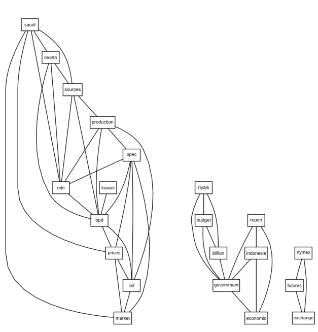
market oil prices bpd mln opec production sources kuwait month economic government indonesia report saudi billion budget riyals exchange futures nymex
Figure 6: Visualization of the correlations within a term-document matrix.
oil opec 1.00 0.87
Internally we compute the correlations between all terms in the term-document matrix and filter those out higher than the correlation threshold.
Figure6shows a plot of the term-document matrixcrudeTDMwhich visualizes the correlations over 0.5 between frequent (co-occurring at least 6 times) terms.
Conceptually, those terms with high correlation to the given term oilcan be interpreted as its valid associations. From the example we can see thatoilis highly associated withopec, which is quite reasonable. As associations are based on the concept of similarities between objects, other similarity measures could be used. We use correlations between terms, but
theoretically we could use any well defined similarity function (confer to the discussion on the dissimilarity()function in the next section) for comparing terms and identifying similar ones. Thus the similarity measures may change but the idea of interpreting similar objects as associations is general.
5.2. Simple text clustering
In this section we will discuss classical clustering algorithms applied to text documents. For this we combine our known acq and crude data sets to a single working set ws in order to use it as input for several simple clustering methods
R> ws <- c(acq, crude) R> summary(ws)
A text document collection with 70 text documents
The metadata consists of 2 tag-value pairs and a data frame Available tags are:
merge_date merger
Available variables in the data frame are: MetaID
Hierarchical clustering
Here we show hierarchical clustering (Johnson 1967; Hartigan 1975; Anderberg 1973; Har-tigan 1972) with text documents. Clearly, the choice of the distance measure significantly influences the outcome of hierarchical clustering algorithms. Common similarity measures in text mining are Metric Distances, Cosine Measure, Pearson Correlation and Extended Jaccard Similarity (Strehl et al. 2000). We use the similarity measures offered by dist from package proxy (Meyer and Buchta 2007) in ourtm package with a generic custom distance function dissimilarity()for term-document matrices. So we could easily use as distance measure the Cosine for ourcrudeterm-document matrix
R> dissimilarity(crudeTDM, method = "cosine")
Our dissimilarity function for text documents takes as input two text documents. Internally this is done by a reduction to two rows in a term-document matrix and applying our custom distance function. For example we could compute the Cosine dissimilarity between the first and the second document from ourcrude collection
R> dissimilarity(crude[[1]], crude[[2]], "cosine") 127
144 0.4425716
In the following example we create a term-document matrix from our working set of 70 news articles (Data() accesses the slot holding the actual sparse matrix)
crude crude crude crude crude crude crude crude
acq
crude acq acq acq acq acq acq acq acq acq acq acq acq acq acq acq acq acq crude acq acq acq acq acq acq acq acq acq acq acq crude crude
acq acq acq acq acq acq acq acq acq acq acq
crude
acq acq acq acq acq acq
acq acq crude crude crude crude
acq
crude crude acq crude
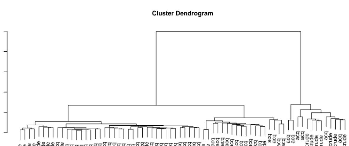
0 50 100 150 200 250 Cluster Dendrogram hclust (*, "ward") dist(wsTDM) Height
Figure 7: Dendrogram for hierarchical clustering. The labels show the original group names.
R> wsTDM <- Data(TermDocMatrix(ws))
and use the Euclidean distance metric as distance measure for hierarchical clustering with Ward’s minimum variance method of our 50acqand 20 crudedocuments:
R> wsHClust <- hclust(dist(wsTDM), method = "ward")
Figure7visualizes the hierarchical clustering in a dendrogram. It shows two bigger conglom-erations ofcrude aggregations (one left, one at right side). In the middle we can find a big acqaggregation.
k-means clustering
We show how to use a classical k-means algorithm (Hartigan and Wong 1979; MacQueen 1967), where we use the term-document matrix representation of our news articles to provide valid input to existing methods inR. We perform a classical linear k-means clustering with
k = 2 (we know that only two clusters is a reasonable value because we concatenated our working set of the two topic setsacqand crude)
R> wsKMeans <- kmeans(wsTDM, 2)
and present the results in form of a confusion matrix. We use as input both the clustering result and the original clustering according to the Reuters topics. As we know the working set consists of 50acqand 20crude documents
R> wsReutersCluster <- c(rep("acq", 50), rep("crude", 20))
Using the functioncl_agreement()from packageclue(Hornik 2005,2007a), we can compute the maximal co-classification rate, i.e., the maximal rate of objects with the same class ids in
both clusterings—the 2-means clustering and the topic clustering with the Reutersacq and crudetopics—after arbitrarily permuting the ids:
R> cl_agreement(wsKMeans, as.cl_partition(wsReutersCluster), "diag") Cross-agreements using maximal co-classification rate:
[,1] [1,] 0.7
which means that thek-means clustering results can recover about 70 percent of the human clustering.
For a real-world example on text clustering for the tm package with several hundreds of documents confer toKaratzoglou and Feinerer(2007) who illustrate that text clustering with a decent amount of documents works reasonably well.
5.3. Simple text classification
In contrast to clustering, where groups are unknown at the beginning, classification tries to put specific documents into groups known in advance. Nevertheless the same basic means can be used as in clustering, like bag-of-words representation as a way to formalize unstructured text. Typical real-world examples are spam classification of e-mails or classifying news articles into topics. In the following, we give two examples: first, a very simple classifier (k-nearest neighbor), and then a more advanced method (Support Vector Machines).
k-nearest neighbor classification
Similar to our examples in the previous section we will reuse the term-document matrix representation, as we can easily access already existing methods for classification. A possible classification procedure isk-nearest neighbor classification implemented in theclass(Venables and Ripley 2002) package. The following example shows a 1-nearest neighbor classification in a spam detection scenario. We use the Spambase database from the UCI Machine Learning Repository (Asuncion and Newman 2007) which consists of 4601 instances representingspam andnonspame-mails. Technically this data set is a term-document matrix with a limited set of terms (in fact 57 terms with their frequency in each e-mail document). Thus we can easily bring text documents into this format by projecting our term-document matrices onto their 57 terms. We start with a training set with about 75 percent of the spam data set resulting in about 1360spamand 2092nonspam documents
R> train <- rbind(spam[1:1360, ], spam[1814:3905, ])
and tag them as factors according to our know topics (the last column in this data set holds thetype, i.e., spam ornonspam):
R> trainCl <- train[, "type"]
In the same way we take the remaining 25 percent of the data set as fictive test sets R> test <- rbind(spam[1361:1813, ], spam[3906:4601, ])