Brain MR Image Segmentation: From Multi-Atlas Method To Deep Learning Models

(1)

University of Windsor University of Windsor

Scholarship at UWindsor

Electronic Theses and Dissertations Theses, Dissertations, and Major Papers

Summer 6-27-2019

Brain MR Image Segmentation: From Multi-Atlas Method To Deep

Learning Models

Jie Huo

University of Windsor

Follow this and additional works at: https://scholar.uwindsor.ca/etd

Recommended Citation Recommended Citation

Huo, Jie, "Brain MR Image Segmentation: From Multi-Atlas Method To Deep Learning Models" (2019). Electronic Theses and Dissertations. 7768.

https://scholar.uwindsor.ca/etd/7768

This online database contains the full-text of PhD dissertations and Masters’ theses of University of Windsor students from 1954 forward. These documents are made available for personal study and research purposes only, in accordance with the Canadian Copyright Act and the Creative Commons license—CC BY-NC-ND (Attribution, Non-Commercial, No Derivative Works). Under this license, works must always be attributed to the copyright holder (original author), cannot be used for any commercial purposes, and may not be altered. Any other use would require the permission of the copyright holder. Students may inquire about withdrawing their dissertation and/or thesis from this database. For additional inquiries, please contact the repository administrator via email

(2)

BRAIN MR IMAGE SEGMENTATION:

FROM MULTI-ATLAS METHOD TO DEEP LEARNING

MODELS

by

Jie Huo

A Dissertation

Submitted to the Faculty of Graduate Studies

through the Department of Electrical and Computer Engineering in Partial Fulfillment of the Requirements for

the Degree of Doctor of Philosophy at the University of Windsor

Windsor, Ontario, Canada c

(3)

BRAIN MR IMAGES SEGMENTATION:

FROM MULTI-ATLAS METHOD TO DEEP LEARNING

MODELS

by Jie Huo APPROVED BY:

P.Atrey, External Examiner

University at Albany, State University of New York

R. Gras

School of Computer Science

H. Wu

Department of Electrical and Computer Engineering

E. Abdel-Raheem

J. Wu, Advisor

(4)

Declaration of Co-Authorship / Previous

Publication

I Co-Authorship Declaration

I hereby declare that this dissertation incorporates material that is result of joint research, as follows: This dissertation also incorporates the outcome of a research under the supervision of professor Jonathan Wu and collaboration with Dr. Guanghui Wang (Chapter 3, Chapter 4), Dr. Akilan Thangarajah (Chapter 3) and Dr. Jiuwen Cao (Chapter 4). The research under Jonathan Wu is covered in Chapter 4, 5, 6, and 7 of the dissertation. In all cases, the key ideas, primary contributions, experimental designs, data analysis, interpretation, and writing were performed by the author, and the contribution of the co-authors was primarily through the provision of proof reading and reviewing the research papers regarding the technical content.

I am aware of the University of Windsor Senate Policy on Authorship and I certify that I have properly acknowledged the contribution of other researchers to my disser-tation, and have obtained written permission from each of the co-authors to include the above materials in my dissertation.

I certify that, with the above qualification, this dissertation, and the research to which it refers, is the product of my own work.

II Previous Publication

This dissertation includes four original papers that have been previously published/un-der review in peer reviewed journals and conferences, as follows:

Thesis

Chapter Publication title/full citation

Publication status

Chapter 3

J. Huo, G. Wang, QM. Wu, and T. Akilan “Label fusion for multi-atlas segmentation based on majority voting.” International Conference Image Analysis and Recogni-tion, pages 100106. Springer, 2015.

Published Chapter 4

J. Huo, QM. Wu, J. Cao, and G, Wang “Supervoxel based method for multi-atlas segmentation of brain MR images.” NeuroImage, 175:201-214, 2018

(5)

Chapter 5

J. Huo and QM. Wu “AttentionNet: brain anatomical structure segmentation using CNN with attention mech-anism.”

Under prepara-tion for submission Chapter 6 J. Huo and QM. Wu, “End-to-end trainable CNN-CRF

with high order potentials.”

Under prepara-tion for submission I certify that I have obtained a written permission from the copyright owner(s) to include the above published material(s) in my thesis. I certify that the above ma-terial describes work completed during my registration as a graduate student at the University of Windsor.

III General

(6)

Abstract

Quantitative analysis of the brain structures on magnetic resonance (MR) images plays a crucial role in examining brain development and abnormality, as well as in aiding the treatment planning. Although manual delineation is commonly considered as the gold standard, it suffers from the shortcomings in terms of low efficiency and inter-rater variability. Therefore, developing automatic anatomical segmentation of human brain is of importance in providing a tool for quantitative analysis (e.g., volume measurement, shape analysis, cortical surface mapping). Despite a large number of existing techniques, the automatic segmentation of brain MR images remains a challenging task due to the complexity of the brain anatomical structures and the great inter- and intra- individual variability among these anatomical structures.

(7)

Dedication

(8)

Acknowledgements

I would like to express my special appreciation and thanks to my advisor, Dr. Q.M. Jonathan Wu for giving me the opportunity to work under his supervision as well as for his guidance and continuous support for my Ph.D. study and research. Additionally, I like to thank the committee members, Dr. Robin Gras, Dr. Esam Abdel-Raheem, and Dr. Huapeng wu for taking time out of their busy schedule to come over and help me with their insightful comments and encouragement. I like to convey my sincere gratitude to Dr. Guanghui Wang, who helped me to learn the fundamental items of the machine learning domain. Furthermore, I sincerely appreciate the department graduate secretary Ms. Andria Ballo for all her support and guidance.

I sincerely thank my beloved husband, Chen, who continuously motivated me and supported me throughout my Ph.D. program. Words cannot express how grateful I am to my mother, father, my mother-in-law, and father-in-law for all of the sacrifices that they have made on my behalf. I thank my fellow labmates for the stimulating discussions and for all the fun we have had in the last few years.

(9)

List of Tables

4.1 A complete list of features used in this work. . . 49 4.2 Dice coefficients of different components analysis. . . 58 4.3 Dice coefficient and running time of four baseline methods and the

pro-posed method on three public datasets. . . 60 4.4 Dice coefficient of using different registration strategies . . . 64 5.1 Architecture of the Attn-Resnet-50. . . 78 5.2 Dice coefficients of LPBA40 for Attn-Resnet-50 at different settings of

Nk. Unique block size Nk = 12 is the baseline. Compared with the

baseline, the staircaseNk, uniqueNk = 22, and uniqueNk = 42achieve

significant improvement, according to two-sided, paired t-test (**p <

0.005,*p < 0.001). . . 82 5.3 Dice coefficients, parameter numbers, and the inference time of 2D slice

of nine architectures with different up-sampling variants and feature combination variants. On validation data, the Attn+ResBlock achieves a significant improvement over the other eight nets in validation Dice coefficients, according to a paired, two-sided t-test (p <0.001). . . . 87 5.4 Comparison of encoder nets on LPBA40 dataset, including the parameters

of the encoder, mean Dice coefficients on validation data, and inference time per coronal slice. The 8x up-sampling scheme in FCN (FCN-8s) is used as the baseline. . . 89 5.5 Validation Dice coefficients and inference time of each 3D image of the

proposed AttentionNet with the state-of-the-art architectures on IBSR. 92 6.1 Mean Dice coefficients of different settings of the average size of the

(14)

6.3 Per-class and mean Dice coefficient comparison on the LPBA dataset, where left and right hemisphere labels are shown jointly. The proposed CNN-HOCRF yields significant improvement comparing with the other four models, according to two-sided, paired t-test on the Dice coefficient

(p <0.001). . . 109

(15)

List of Figures

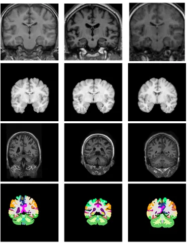
1.1 2D slice examples of the MR images for brain anatomical segmentation. 1st row, 2nd row, and 3rd row are the intensity images from three datasets; the last row shows the corresponding label images of the 3rd

row. . . 5

2.1 Building blocks of multi-atlas segmentation [50] (Dashed blocks are op-tional steps). . . 11

2.2 Directly applying classification net to segmentation task. [39] . . . 20

2.3 FCNN architecture with parallel convolutional pathways. [61] . . . 21

2.4 Architecture of U-net. [87] . . . 21

2.5 Three planes of a brain MR image. . . 23

3.1 Illustration of labeling for the target patch, where red square in target im-age denotes the target patch; the blue, pink and green squares in atlas image indicate patches in a searching window; and the best matched patch in each atlas is shown as red squares. . . 29

3.2 Hippocampus segmentation performance using different patch radius and searched patch radius. . . 33

3.3 Sagittal views of the segmentations produced by different patch radius and searched patch radius. Where the red region shows the overlap between the automatic and the manual segmentation; the green region is the manual segmentation; and the blue region is automatic segmentation using the proposed method. . . 34

(16)

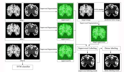
4.1 Framework overview of the proposed method. Supervoxel segmentation is performed on the target and the registered atlas images, respectively. The supervoxel labeling corresponds to a supervoxel-based graphical model. The dense labeling relates to a grid graphical model, aiming at refining the supervoxel labeling results. The SVM classifier is used to generate the predicted label image of the target for supervoxel seg-mentation and the probability map for initialization of data term in dense labeling. . . 41 4.2 An example of slices in the axial plane, sagittal plane, and coronal plane

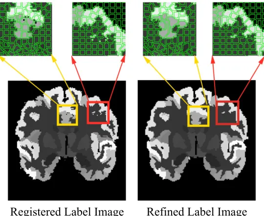
of the label image. Non-smooth tissue boundaries are displayed in the axial and sagittal plane. . . 42 4.3 A comparison of the label image before (left) and after (after) the

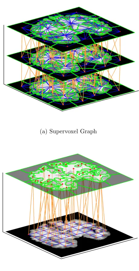
refine-ment scheme. Before performing the refinerefine-ment scheme, the registered label image demonstrates isolated holes which cause label inconsistency within the supervoxel. After applying the refinement scheme, the iso-lated holes in the label image are filled, and the label consistency is enforced within the supervoxel. . . 43 4.4 Three consecutive slices are shown for the supervoxel graph (a), where

the blue edges E1 indicate the pairwise potential in the coronal plane

while the orange edges E2 are the pairwise potential of two adjacent

slices. The dense graph (b) takes one slice as an example, where the bottom layer and top layer illustrate the grid graph and supervoxel layer, respectively. The blue edges indicate the pairwise potential in the grid graph while the orange edges show the high order potential. The nodes are indicated with red dots in both graphs. . . 47 4.5 Influence of parameters γ and cin the SVM on classification accuracy. . 53 4.6 Supervoxel segmentation results of using SLIC based on (a) intensity

im-age, (b) feature image using a concatenation of the texture feature, coordinates and intensity, and (c) predicted label image obtained from the SVM classifier. . . 53 4.7 Supervoxel segmentation performance with respect to k. (a) and (c)

in-dicate the averaged accuracy and processing time for supervoxel seg-mentation (error bar at ±1 std), respectively. (b) demonstrates the averaged segmentation accuracy for the dense labeling (error bar at

(17)

4.8 Supervoxel segmentation on the ground truth image with different super-voxel size k. . . 56 4.9 Overall accuracy in terms of mean Dice coefficient, with respect to the

number of the atlases (error bar at ±1 std). . . 56 4.10 Segmentation results of the different components analysis. . . 58 4.11 Per-label accuracy comparison on the whole brain segmentation using

three public datasets where the left and right hemisphere labels are shown jointly. The proposed method is compared with four baseline methods in the experiment. . . 62 4.12 Segmentation results of the MICCAI 2012, the LPBA40, subcortical

la-bels of IBSR, and cortical lala-bels of IBSR datasets. Common mistakes (indicated by arrows) of the baseline methods include 1) spatial in-consistency in MICCAI 2012; 2) excessive smoothness of boundaries in LPBA40; 3) excessive smoothness in tiny structures in subcortical labels of IBSR; and 4) spatial inconsistency in cortical labels of IBSR. 63 5.1 General encoder-decoder architecture for image segmentation. . . 72 5.2 Building block of the spatial attention model. . . 73 5.3 Building block of the spatial attention function. . . 74 5.4 A toy example of the 2D attention model. For queries (1,4,4, dk) and keys

(1,8,8, dk), they are partitioned into 2×2 query/key blocks, where the

query block size is 2×2 and the key block size is 4×4. By performing the spatial attention function on the query block and the corresponding key block, we obtain a weight map with a size of 8×32. The weight map contains 2×2 sub weight maps, where each sub weight map with the size of 4×16 indicates the similarity scores of the query vectors and key vectors in the corresponding query and key block. . . 76 5.5 Structure of the residual upsampling block. . . 77 5.6 Coronal image augmented by the relative coordinates: (a) x, (b) y, (c) z.

(d) is the original coronal image without position information. . . 79 5.7 Visualization of the weights maps of three attention layers with different

settings of Nk. Column 4 indicates the details of the red square in

(18)

5.8 Training behavior of nine architectures on training data (left column) and validation data (right column). The nine architectures share the same encoder net and vary the decoder net and the feature combination unit. The up-sampling units are residual upsampling block (ResBlock), deconvolution up-sampling unit (Deconv), and U-net up-sampling unit (UnetDec). Also, the feature combination units are spatial attention model (Attn), addition (Add), and concatenation (Concat). . . 86 5.9 Visual quality comparison of (a) different feature combination methods,

(b) different up-sampling units. In (a), area A and C show that the attention outperforms concatenation and addition in predicting the details; area B demonstrates the common mistake made by the three methods; arrows refer to the “isolated regions” predicted by the con-catenation and addition. In (b), area A illustrates that ResBlock yields better segmentation performance; area B is the common mistake of the three up-sampling units. . . 88 5.10 Examples of segmentation results on the IBSR dataset. . . 91 6.1 Building block of one iteration of the mean field approximation algorithm,

¯

Q=Q

j∈c,j6=iQj(xj =l). . . 101

6.2 Architecture of the proposed CNN-HOCRF. . . 102 6.3 Dice coefficients w.r.t. the number of mean field iterations . . . 105 6.4 Comparision of the segmentation results of three coronal slices on LPBA40.

Refer to [97] for color index. . . 110 6.5 Learned parameters of µand wh. The adjacent rows (columns) in the

(19)

List of abbreviation

2D Two-Dimension or Two-Dimensional

3D Three-Dimension or Three-Dimensional

BN Batch Normalization

CNN or ConvNet Convolutional Neural Network

CRF Conditional Random Field

EM ExpectationMaximization

FCN Fully Convolutional Network

JLF Joint Label Fusion

LMFB Leung-Malik Filter Banks

MAP Maximum-A-Posteriori

MRF Markov Random Field

MRI Magnetic Resonance Imaging

MR Magnetic Resonance

MV Majority Voting

PB Patch-Based

RBF Radial Basis Function

ReLU Rectified Linear Unit

RDA Regularized Dual Averaging

ROI Region Of Interest

SLIC Simple Linear Iterative Clustering

SVM Support Vector Machine

SVMAF SVM Segmentation with Augmented Features

SSD Summed Squared Distance

STAPLE Simultaneous Truth and Performance Level Estimation

(20)

Chapter 1 Introduction

In this chapter, we start with introducing the topic of this Ph.D. dissertation — anatomical structure segmentation of the brain MR images in Section 1.1. Next, the motivation of the study and the research challenges related to the brain anatomical segmentation are presented in Section 1.2 and Section 1.3, respectively. Then, we clarify the contributions of the work in Section 1.4. Finally, the structure of this dissertation is explained in Section 1.5.

1.1 Segmentation of Brain MR Images

As an essential task in medical image analysis, segmentation aims at providing each pixel/voxel a label which refers to the tissue or the anatomical structure. The seg-mentation result is either a set of contours describing the region boundaries or an image of labels which identifies each homogeneous region [29]. The brain segmenta-tion problem discussed in this thesis mainly focuses on brain anatomical structure segmentation, which relates to assigning each pixel/voxel in the image with a label associated with an anatomical structure in the brain.

(21)

struc-tural changes in the brain, resulting in volume or shape alternations in magnetic resonance (MR) images. Accurate brain anatomical segmentation is widely used to study the morphometric changes or to measure the volume for characterizing the neurological disorders. Moreover, segmentation not only contributes to examine the brain development and abnormality but also plays an important role in detection and localization of the abnormal tissues and surrounding healthy structures, which is an essential task for surgical planning, postoperative analysis, and chemo/radio-therapy planning [2, 54]. In addition, the segmented brain usually serves as the preliminary step of many brain image analysis, such as cortical surface mapping [38] and brain images registration and warping [96], of which the performance directly influences the outcome of following procedures. Except for the clinical applications, the anatomically segmented brain also provides a framework of functional visualiza-tion and quantitive analysis for studying and analyzing the abnormalities such as neurodegenerative disorder, psychiatric disorders, and healthy aging.

Magnetic resonance imaging (MRI) is an imaging technology that produces three-dimensional detailed anatomical images. Since the MRI offers high-resolution images and shows high contrast between soft tissues, MRI becomes the most popular medical imaging modality used for quantitive and qualitative analysis of the brain structures. Therefore, anatomical segmentation on brain MR images provides an effective tool for the anatomical and functional study of the brain.

1.2 Motivation

Because of the crucial role that segmented brain MR images play in research and clin-ical applications, precise anatomclin-ical segmentation becomes an essential prerequisite for the quantitative assessment of the brain.

(22)

consid-ered as the “gold standard”. However, the manual annotation can take up to a week for high-resolution MR images [35]. Moreover, it suffers from the shortcoming of intra- and inter-rater variability [24]. As a result, the manual segmentation is prone to errors and difficult to reproduce. Therefore, the manual delineation is not suitable for deploying on large-scale datasets or in applications where time is critical [50].

On the other hand, some fully-automated algorithms, e.g., thresholding, region growing, clustering methods, yield high accuracy in specific problems. Generally, the fully-automated algorithms rely on the intensity information of the MR images to classify the pixel/voxel or utilize a probabilistic atlas which stores the spatial infor-mation to aid the intensity-based segmentation. Unfortunately, these fully-automated algorithms only work for some specific segmentation tasks, e.g., tissue classification of gray matter (GM), white matter (WM), and cerebrospinal fluid (CSF) [35], while they are not applicable to the detailed segmentation due to the overlap of intensity profiles for the complicated anatomical structures of the brain. Moreover, the perfor-mance of the fully-automated methods is limited by the artifacts in the MR images, including intensity inhomogeneity, noise, and partial volume [29].

(23)

1.3 Challenges

Brain anatomical segmentation is a challenging task despite significant efforts made by scientists and researchers. Figure 1.1 depicts some 2D slices of the brain images and label images, which reflects the challenges in brain anatomical segmentation. In this section, we present several research challenges for the field of brain anatomical structure segmentation.

Intensity overlap. MR signal holds the properties to differentiate brain and

nonbrain tissues or even to distinguish among GM, WM, and CSF. Some methods thus achieve competitive performance [34, 102] in basic tissue classification (i.e., GM, WM, and CSF) or brain extraction (i.e., brain and non-brain tissue). However, as shown in Figure 1.1, the intensity overlap between distributions of different anatomical structures is severe, especially in the cortical area.

Large variations in shape, size, appearance. The shape, volume, and

ap-pearance of the anatomical structures relate to the gender, age, and pathological conditions with tumors, lesions, and edemas. These factors result in significant intra-class variations among different subjects. For example, as shown in Figure 1.1, there are considerable variations in the appearance, shape, and the size of the brain anatom-ical structures among different subjects. Moreover, the quality of the MR images is also affected by the scanner, machine, and even acquisition time.

Complicated labeling protocol. Compared with the basic tissue classification

(24)

(25)

becomes an obstacle for some learning-based methods.

Spatial and contextual information. The spatial information plays an

essen-tial role in brain anatomy. Given a position in the brain, the number of the possible classes for the voxel is very limited. As a result, involving the position prior is a crucial point for successful segmentation of the brain anatomical structure. Moreover, the relative positions of the brain anatomical structures are fixed, e.g., the amygdala is anterior and superior to the hippocampus; structures of the left hemisphere and right hemisphere are rarely in the adjacent regions. Therefore, learning or interpreting this contextual relation also contributes to improving the segmentation performance.

Precise boundaries. Limited by the confounding appearance and the

compli-cated labeling protocol, it is rather challenging to obtain a precise boundary for each anatomical structure. Moreover, the training data is usually too small to cover the various pattern of structure appearance. Therefore, the detailed prediction is the most challenging task for the brain anatomical segmentation problem.

Labeling inconsistency. As for the anatomical segmentation, the labeling

within the neighborhood should be homogeneous. However, the labeling inconsis-tency problem is common in the segmentation results produced by some learning-based methods, e.g., support vector machine (SVM) and random forest. For the deep learning based methods, e.g., convolutional neural network (CNN), the labeling in-consistency is alleviated, however, the segmentation is usually followed by a graphical model, e.g., Markov random field (MRF) and conditional random fields (CRF), to refine the inconsistent labeling results.

1.4 Objective and Contributions

(26)

segmen-tation, including a two-stage majority voting scheme, a supervoxel based graphical model, a CNN with attention mechanism, and an end-to-end trainable network which combines CNN with high order CRF. This section enlists the major contributions of this dissertation as follows:

1. We develop a novel two-stage majority voting framework for multi-atlas seg-mentation of hippocampus on brain MR images. The first majority voting fuses the atlas labels at the image patch level with sliding a window across the target image, followed by the second majority voting which fuses the results of the first voting for the overlapping positions. We experimentally demon-strated the effectiveness of the two-stage majority voting strategy in avoiding the over-segmentation problem by comparing with the original voting scheme. 2. We propose a supervoxel based graphical model for brain anatomical

segmen-tation. Supervoxel is an aggregation of voxels with similar attributes. Based on the assumption that the voxels within the same supervoxel have the same label, we construct the graphical model on the supervoxels. By minimizing the en-ergy function associated with the supervoxel based graphical model, the dense labeling of MR image is converted to the supervoxel labeling problem. Since supervoxels are considered as the nodes in the graphical model, the number of variables is much less than the graphical model defined on voxels, resulting in short inference time. Moreover, because all the voxels inside the supervoxel are assigned the same label, the labeling consistency is thus encouraged within the supervoxel.

(27)

spatial positions in the finer feature maps. By combining the related finer fea-tures with the high-level feafea-tures, the net is equipped with the ability of precise localizing and detailed boundaries prediction.

4. We develop a 2D CNN architecture, which benefits the model in terms of low memory requirement, deep architecture, and fine-tuning on the pre-trained model. In order to deal with the 3D data format in MR images, we embed the spatial position information along with the intensity images in the inputs. The incorporation of the position information not only compensates for the loss of the spatial context in the third dimension but also enables the net to train on both intensity and spatial prior.

5. We propose a unified framework which combines the strength of CNN with high order CRF. Considering the characteristic of brain anatomical structures, we propose a semi-densely connected pairwise potential which encourages the smoothness of the labeling between two pixels within a neighborhood. In ad-dition, we apply a class-specific kernel weight to the high order potential. We derive the mean field approximation for the high order CRF and model the in-ference as building blocks of CNN so that the CNN and high order CRF can be trained in an end-to-end fashion where the parameters are learned jointly dur-ing the traindur-ing phase. By employdur-ing the superpixel based high order term, the proposed high order CRF encourages the labeling consistency among the pixels within the same superpixel. Extensive experiments demonstrate that involving the high order potential contributes to improving the segmentation accuracy compared with the other graphical models.

1.5 Organization of Thesis

(28)

(29)

Chapter 2 Background

2.1 Overview

For anatomical segmentation of the brain MR images, the existing methodologies can be categorized into three groups: multi-atlas segmentation, graphical model, and learning based method. In this chapter, we review the related works regarding the three methods along with the corresponding background knowledge.

2.2 Multi-atlases Segmentation

2.2.1 Background

Atlas-guided segmentation is a widely used method for the neuroanatomical structure segmentation. By registering the target image to the manually labeled image, one can obtain a mapping between two coordinate systems which can be used to transfer the labels from the atlas to the target image. This technique refers to the classic single-atlas segmentation procedure. However, the single single-atlas is not capable of dealing with the wide anatomical variation. Consequently, instead of the single atlas, multiple atlases are employed for brain anatomical structure segmentation.

(30)

Figure 2.1: Building blocks of multi-atlas segmentation [50] (Dashed blocks are op-tional steps).

(31)

2.2.2 Related Work

Registration. In multi-atlas segmentation, registration is in charge of

establish-ing the spatial correspondence between the target image and each atlas. Based on the geometric transformation, it can be divided into rigid and non-rigid registration. Rigid registration is usually applied to rigid structures, e.g., bones, or employed as a pre-registration strategy. For brain anatomical structures, the multi-atlas segmenta-tion methods usually adopt complex deformable models which assign each locasegmenta-tion a spatial transformation vector, such as nonlinear deformable models [42, 86] or non-parametric diffeomorphisms [15, 110].

For multi-atlas segmentation, since the registration is performed between the tar-get and each atlas pairwisely, the registration step becomes the computational bottle-neck. Some methods can reduce the computational burden of the pairwise registration by reducing the number of atlases [124]. Alternatively, some research co-registered all the atlases to construct a template atlas. By performing the registration between the target and the template atlas, this approach can reduce the computation cost of regis-tration but also might lead to the decrease of the performance due to the suboptimal registrations [4, 98]. Moreover, the patch-based technique searches the neighborhood in the atlas and thus relax the one-to-one correspondence assumption in multi-atlas segmentation. Therefore, patch-based methods can be combined with the multi-atlas segmentation for alleviating the requirements for high accurate pairwise registration. [8, 13, 88, 116].

Label fusion. In multi-atlases segmentation, the segmentation errors stem from

(32)

utilizes the global information and associate each atlas with a unique weight which is estimated by comparing the mutual information [6] or by posing it as a least square problem [18]. However, the global weight cannot explain the spatial variety. Instead, local weighted fusion methods are developed to use local similarities between the atlas and the target (e.g., local absolute difference [55], local cross-correlation [7], Gaussian intensity difference function[58], and Jacobian determinant of the deformation fields [85]). Wang et al. [117] developed the joint label fusion to account for the correlations of label errors produced by different atlases in the voting strategy. The weights are optimized to minimize the total expected segmentation error, which relates to the pairwise dependencies among the atlases.

Sabuncu et al. [91] proposed a generative model for label fusion, which is formu-lated by marginalizing the conditional probability with respect to a mapping field. By configuring the mapping field, the model evolves into different label fusion algo-rithms and generalize the global and local weighted fusion methods. Based on this generative probabilistic model, Iglesias et al. [51] applied a joint histogram instead of the Gaussian noise in [91], extending the generative model to intermodality fusion; Bai et al. [13] integrated the patch-based method with the generative model, leading to a probabilistic patch-based label fusion.

In addition, another category of probabilistic label fusion methods is established on the simultaneous truth and performance level estimation (STAPLE) [120], which integrates a stochastic model of rater behavior into the estimation process. Many works have been developed in modifying the original probabilistic model, including defining data-driven a priori distribution [70], introducing a hierarchical noise model [9], and integrating non-local correspondence into the STAPLE framework [8].

(33)

patch-based technique can be incorporated into the label fusion scheme and account for the registration errors.

2.3 Random Field for Segmentation Problem

2.3.1 Background

The segmentation problem can be posed as a MAP estimation for an appropriately de-fined graphical model which is associated with a CRF [65, 68, 99]. Given an imageI, a random field is defined over a set of random variablesX ={X1, X2, . . . , XN}, where

each random variable is associated with a corresponding image pixeli∈ {1,2, . . . , N}

and takes a value from the label setL={l1, l2. . . , lk}. The CRF (X, I) is

character-ized by a Gibbs distribution:

P(X|I) = 1

Z(I)exp

−X

c∈C

ψc(Xc |I)

(2.1) where the partition functionZ(I) is a normalizing constant, cliquecis a set of random variables that are conditionally dependent on each other,C is the set of all the cliques, andψcis the potential term induced by the cliquec. The Gibbs energy of the labeling

configuration x∈ LN _is:

E(x) =X

c∈C

ψc(xc) (2.2)

where notation of conditioning on Iis omitted for convenience. Therefore, the MAP labeling of the random field in Equation (2.1) corresponds to minimizing the Gibbs energy function in Equation (2.2).

Based on the definition of the cliques and the corresponding potentials, the CRF model can be divided into three models:

Adjacency CRF: In the adjacency CRF model, the clique set C involves the

unary cliques and the pairwise cliques. The energy function is:

E(x) = X

i∈V

ψu(xi) +

X

i∈V,j∈N

(34)

Each unary clique is associated with a random variable Xi, the corresponding unary

potential ψu measures the cost of assigning label xi to pixel i. The pairwise clique

consists of a pair of random variables,Xi and its neighborXj. The pairwise potential

ψp measures the cost of assigning label xi and xj to pixel i and j simultaneously.

Fully connected CRF: The only difference between adjacency CRF and fully

connected CRF is that the fully connected potentials are defined over all the pixel pairs in the image instead of a neighborhood system. The energy function is:

E(x) =X

i∈V

ψu(xi) +

X

i<j

ψp(xi, xj) (2.4)

High order CRF: Besides unary cliques and pairwise cliques, the high

or-der CRF involves the high oror-der clique which refers to a set of variables Xs =

{X1, X2, . . . , XM}. The high order CRF is of the form:

E(x) =X

i∈V

ψu(xi) +

X

i,j

ψp(xi, xj) +

X

c∈S

ψh(xc) (2.5)

where the high order potentialψh measures the cost of the label configuration xs for

the set of variables and S denotes the set of all the high order cliques. The pairwise potentials can be defined over the neighborhood system or the whole image.

2.3.2 Related Work

The graphical model has been successfully applied to brain anatomical structure seg-mentation [93, 108]. By employing a graphical model defined on voxels, one can obtain the optimal label for each voxel by minimizing the corresponding energy function. In these approaches, the prior knowledge is usually obtained by registering the target to a fixed probabilistic atlas1. Those approaches can be categorized as fully-automated

1 _{probabilistic atlas is an anatomical template that retains quantitative information on inter-subject}

(35)

algorithms, which are not in the scope of review in this thesis. In this section, we focus on the methods that combine the graphical model with the multi-atlas segmentation. Regarding combining the graphical model with the multi-atlas segmentation, some methods employ the graphical model as a post-processing step following the label fusion to refine the labeling results [107]. With employing the probabilistic map obtained from the label fusion step as the spatial prior, the corresponding energy can be minimized by using graph-cuts [76, 121], or max-flow [64, 84].

Alternatively, the graphical model can serve as the registration between the tar-get and the atlas, which turns to minimize the energy function with respect to the displacement vector [36, 43]. Moreover, some works integrate the registration and segmentation in one graphical model to solve the registration and segmentation si-multaneously. Alchatzidis et al. [3] designed the MRF energy function comprising registration term and segmentation term and optimized it through dual decomposi-tion algorithm. Gass et al. [37] cast the simultaneous segmentadecomposi-tion and registradecomposi-tion problem as a two-layer graph defined on MRF and developed hierarchical implemen-tation, allowing coarse-to-fine registration and pixelwise label estimation.

(36)

within the supervoxel have the same label so that accurate supervoxel segmentation is a prerequisite. However, this requirement is difficult to achieve due to the intensity overlap in different anatomical structures and the lack of visible boundaries in some ROIs, especially in the cortical area. As a result, the supervoxel graphical model is usually applied to the tumor segmentation [53] or subcortical area segmentation instead of cortical structure segmentation.

High order potential has demonstrated the effectiveness in computer vision [65, 90, 111, 130]. However, it is unfeasible to compute the general higher-order potential defined over many variables [79], especially for the 3D MR data. In the medical image segmentation field, a few of studies have been proposed to involve the high order potential for encouraging the regional labeling consistency [60], encoding the shape prior [114], or embedding the boundary prior [5].

2.4 Convolutional Neural Network

Brain anatomical segmentation can be viewed as a voxel labeling problem, which makes it possible to employ a classifier (e.g., SVM classifier [12], random forest [132]) to classify the voxel. However, these traditional classifier relies on domain-specific hand-crafted features so that it is difficult to generalize the algorithm among images obtained from different modalities. Recently, due to the success of deep learning in computer vision, increasing deep networks have been developed for medical image segmentation. In this section, the basic knowledge of CNN is first introduced and follows it with the related works of using CNN for brain anatomical segmentation.

2.4.1 Background

(37)

seen as a single differentiable, parameterized function that maps the raw image to class scores. By setting the appropriate loss function, one can update the parameters based on the partial derivatives which are computed through back-propagation.

In order to build CNN, we use the following building blocks in the studies of this thesis.

Convolution layers. Convolutional layers are the core building blocks of the

CNN architecture, which serve as the feature extractors that map data to the trans-formed feature space. It extracts the features by convolving a kernel (or filter) with the inputs. The outputs are usually called feature maps or activation maps. For the convolutional layers, there are three parameters: (1) Kernel size, which refers to the height and weight of the kernel and relates to the receptive field, which is the region of the particular output feature sees from its input space. (2) The depth, which cor-responds to the number of filters that are used for the convolution operation. (3) The stride, which refers to the number of pixels that we jump when sliding the convolution kernel over the inputs. Stride greater than one results in reducing the spatial size.

Fully convolutional layer. To obtain a dense prediction using CNN, we apply

the fully convolutional layer at the top of the architecture. The fully convolutional layer is 1×1 convolution with a depth of L, where L is the number of classes. By appending a fully convolutional layer at the top, one can obtain the class scores at each position simultaneously. However, due to the downsampling operations (e.g., strided convolution or pooling operation), directly applying the fully convolutional layer results in a coarse prediction. Therefore, prior to fully convolution layer, up-sampling operations (e.g., deconvolution layer or interpolation) are usually adopted for applying CNN to segmentation problem.

Deconvolution layer. Deconvolution layer is the transpose of the convolution

(38)

ReLU. As an activation function, ReLU helps a model account for interaction effects and produce the non-linear mapping. The ReLU function has a derivative of 0 for negative inputs while a derivative of 1 for positive inputs, which effectively avoids the vanishing gradient problem.

Batch Normalization. Batch normalization [52] normalizes the output of a

previous activation layer by subtracting the batch mean and dividing by the batch standard deviation. The batch normalization reduces the internal covariate shift that is produced by distribution variation of the layer’s inputs during the training stage, resulting in accelerating the training speed. Moreover, by applying batch normalization layers, the net is more tolerant to increased training rates and often does not require Dropout for regularization.

Softmax function. Softmax function takes a vector of K real numbers as the

input and normalizes it into a probability distribution consisting of K probabilities.

y(z) = e

zi

PK

k=1ezi

(2.6) After applying the softmax function, each element in the vector is normalized to the interval (0,1), and the elements are sum to 1. Thus the output of the softmax function can be interpreted as the probabilities. Furthermore, the softmax function can enlarge the difference between the elements.

It is worth noting that the softmax function has the same formulation as the Gibbs distribution in Equation (2.1), where eachzi can be considered as the energies of the

variable while the denominator is the partition function.

2.4.2 Related Work

(39)

Figure 2.2: Directly applying classification net to segmentation task. [39] Figure 2.2, the networks are trained on 2D/3D image patches cropped from the whole image and produce the prediction of the central position in the image patch. However, during the inference stage, “sliding window” is applied to obtain the pixel/voxelwise prediction, resulting in low inference speed. Moreover, the information redundancy in training patches hinders the performance of the model.

Another approach adopts the 2D/3D fully convolutional network (FCN) archi-tecture [20, 32, 61], which replaces the fully connected layer with the fully convo-lutional layer. The FCN architecture takes inputs with any size and outputs the dense probability map of the input image. In order to capture both local and contex-tual information, architectures with parallel convolutional pathways are employed for multi-scale processing, as illustrated in Figure 2.3. Kamnitsas et al. [61] exploited a two-pathway FCN to take inputs of different resolutions. Havaei et al. [39] adopted two-pathway convolution layers with different convolutional kernel size. The multiple pathway architecture is also prevalent in the voxel/pixel classification net, e.g., in [82], the inputs are of different spatial sizes so that the net is capable of capturing multi-scale context. However, the multiple pathway networks are usually designed in a shallow fashion (two to three convolutional layers followed by fully connected/-convolutional layer) in order to take trade-off between the increasing parameters and memory required for training.

(40)

Figure 2.3: FCNN architecture with parallel convolutional pathways. [61]

Figure 2.4: Architecture of U-net. [87]

net”). The contracting network is topologically identical to a classification net while the expanding network replaces the pooling layers with deconvolution layer to recover the resolution to the input size. The contracting net and expanding net are more or less symmetric, resulting in an u-shape in the appearance of the architecture. Fur-thermore, the local features from the contracting net are connected to the expanding path. The feature combination equips the U-net with the ability to capture both local and larger contextual information. Many works extend the U-net to the spe-cific application by using different loss function [80], using different feature combining methods [127], combining with the state-of-the-art classification networks [33].

(41)

class of a voxel, in the application of brain anatomical structure segmentation, a couple of networks encode the position information into the inputs to augment the segmentation. Wachinger et al. [112] uses the combination of spectral brain coordi-nates and Cartesian coordicoordi-nates. de Brebisson et at. [28] adopts relative coordicoordi-nates which compute the distance from voxel to the centroid of each segmentation. The aforementioned research experimentally demonstrated that the incorporation of the position information leads to improvement in the anatomical structure segmentation. Imbalanced data among different class is a challenging task for brain segmentation even in the other medical image segmentation field. To address this problem, data resampling technique is applied to balance the sample numbers of different classes. Kamnitsas et al. [61] built training batches by cropping the segments with 50% prob-abilities being centered on foreground (tumor) or background (non-tumor) voxel. Havaei et al. [14, 39] adopted a two-phase training strategy to alleviate the class imbalance. In the first training phase, equally sampled training samples are used while the uniformed sampled batches are used in the second training phase with only fine-tuning the last layer. In [112], the authors employed another two-phase training strategy, which separates the brain tissues from the background in the first phase and identifies the anatomical structures in the second phase.

Furthermore, some techniques are applied to deal with the complexity in medical images. For example, integration of multiple modality images leads to significant improvement of the performance [31, 129]. Deep supervision, which adds a group of weighted auxiliary classifiers into the network, is applied by the works in [21, 22, 126] to further strengthen the training process.

2.5 MRI Coordinate System

(42)

stands for right, anterior, and superior, respectively. With three directions left to right, posterior to anterior, and inferior to superior, this space consists of three planes to describe the standard anatomical position of a human:

1. The axial plane is parallel to the ground and separates the superior (head) from the inferior (feet).

2. The coronal plane is perpendicular to the ground and separates the anterior (front) from the posterior (back).

3. The sagittal plane separates the left from the right.

Although there is a difference between the anatomical coordinates and the 3D image coordinates, to simplify the notations in this thesis, we refer the three axises in the volumetric images space asx,y, andz, and represent three planesxy,xz, and

yz as axial slice, coronal slice and sagittal slice, respectively. Figure 2.5 shows the three views of a brain MR image.

(a) Axial view (b) Coronal view (c) Sagittal view

Figure 2.5: Three planes of a brain MR image.

2.6 Datasets

(43)

1. LONI-LPBA40 dataset

The LPBA40 dataset [97] includes 40 T1-weighted MRI scans of healthy volunteers, which is acquired on a GE 1.5T system. The dataset consists of 20 males and 20 females, age 29.20±6.30 years. The 124 coronal brain slices are 1.5 mm apart with in-plane voxel resolution of 0.86 mm (38 subjects) or 0.78 mm (2 subjects). The brain is manually delineated into 50 cortical structures, 4 subcortical areas, the brainstem, and the cerebellum.

2. MICCAI 2012 Multi-Atlas Labeling Challenge dataset

The MICCAI 2012 dataset [69] includes 35 T1-weighted MRI scans obtained from the OASIS project, where 15 subjects (5 males, 10 females, age 23.00±4.12 years) are used as the atlases and the remaining (8 males, 12 females, age 40.40±22.43 years) are used for testing. The labeling protocol for OASIS project is a brain labeling protocol using 134 labels, including 36 subcortical labels and 98 cortical labels.

3. IBSR dataset

The IBSR dataset consists of 18 T1-weighted MRI scans (14 males, 4 females), provided by the Center for Morphometric Analysis at Massachusetts General Hos-pital and are available at http://www.cma.mgh.harvard.edu/ibsr/. Coronal slices are 1.5 mm apart with in-plane resolution of 0.9375 mm (8 subjects), 1 mm (6 subjects), or 0.8371 mm (4 subjects). The IBSR dataset consists of two types of manual segmentation: 1) the images are manually segmented into 32 subcortical structures, and 2) the cortex area is sub-divided into 96 cortical structures.

2.7 Image Pre-Processing

(44)

1. Bias field correction

MR images often exhibit image intensity inhomogeneity that is the result of mag-netic field variations rather than anatomical differences. These artifacts are often described as bias, inhomogeneity, illumination non-uniformity, or gain field, can be produced by imaging instrumentation, such as radio-frequency non-uniformity, and static field inhomogeneity [16, 46]. These variations are often seen as a slowly gained signal that varies spatially. Numerous methods have been proposed to cor-rect this artifact. In this thesis context, the N4 bias field corcor-rection [106] is applied to correct the intensity inhomogeneity.

2. Pairwise registration

In this thesis context, the term ”registration” means to determine the spatial align-ment between two images of different subjects, acquired from the same dataset. Registration relates to a transformation that can associate the position of features in one image or coordinate space with the position of the corresponding feature in another image or coordinate space [45].

In the multi-atlas segmentation, both the intensity images and the label images of the atlases are required to be warped to the target domain with the same transformation. Consequently, the first step of the registration is to generate the transformation files based on the similarity between intensity images of the atlas and the target. Then the transformation files are applied to the atlas intensity image and the label image to generate warped atlas intensity and label image, respectively.

3. Intensity normalization

(45)

(46)

Chapter 3 Label Fusion for Multi-Atlas

Segmentation Based on Majority

Voting

Multi-atlas based segmentation is successfully applied to medical image segmentation. Majority voting, as the simplest label fusion method in multi-atlas based segmenta-tion, is a powerful segmentation method. In this paper, a novel majority voting-based label fusion is proposed by introducing patch-based analysis for automatic segmen-tation of brain MR images. The proposed approach, by comparing the similarity between patches, avoids the over-segmentation problem of majority fusion. The ap-proach is successfully applied to the segmentation of hippocampus, and the experi-mental results demonstrate significant performance improvement over three state-of-the-art approaches in the literature.

3.1 Introduction

(47)

registered to the target image, and voxelwise label conflicts between the registered atlases are resolved by label fusion.

In multi-atlas segmentation, the estimated segmentation is obtained by perform-ing label fusion on the warped atlases. Although weighted fusion and statistical fusion yield good results in segmentation of magnetic resonance (MR) image [105, 118, 122, 123], the estimation of the weight and the expectationmaximization (EM) estimation, which play important roles in weighted fusion and statistical fusion, is very computa-tionally intensive. In contrast, majority voting, which is probably the simplest label fusion method, has been demonstrated to yield powerful segmentation results with less computation. Majority voting method, however, may yield over-segmentation since it does not utilize image intensity information. The patch-based method, which compares the similarity of intensity between patches, can be combined with majority voting multi-atlases segmentation to avoid such over-segmentation errors.

Motivated by this idea, we propose a novel label fusion method which combines majority voting with the patch-based method to achieve automatic segmentation in brain MR images. The proposed method is successfully applied to the segmenta-tion of hippocampus. In addisegmenta-tion, the influences of different parameters are studied empirically, and a comparison with three closely related methods is performed to demonstrate the effectiveness of the proposed approach.

3.2 Method

Consider an imageI ={I(x)|x∈Ω}, wherexdenotes the voxel; and Ω⊂_R3 _denotes

the lattice on which the image is defined. The goal of segmentation is to estimate a label map L associated with the image I, in which each voxel is assigned a discrete labell. The labell takes discrete values from 1 toL for all the possible labels for the voxels in the image. In multi-atlas segmentation, IT is a target image andA1,· · · , An

(48)

Figure 3.1: Illustration of labeling for the target patch, where red square in target image denotes the target patch; the blue, pink and green squares in atlas image indicate patches in a searching window; and the best matched patch in each atlas is shown as red squares.

the target image (Ii is also called warped atlas image); and Si is the corresponding

manual segmentation of this atlas image. After combining the warped atlas images, a fused label map is generated which can be considered as the segmentation of the target image.

(49)

3.2.1 Patch Selection

The performance of atlas-based segmentation can be moderately improved by ap-plying a local searching technique [25]. Although deformable registration has been performed before label fusion, the correspondence obtained from the registration may not guarantee the maximal similarity between the patch in the target image and that in the warped atlas image. Therefore, local searching within a small neighborhood around the voxel in the warped image is performed to achieve the maximal similarity. Summed squared distance (SSD) is used to measure the similarity between the target patch and atlas patch. The SSD of the target patch centered at x and the atlas patch centered at x0 is shown below.

SSD(x, y) =kIT(N(x))−Ii(N(x0))k2 (3.1)

wherex0 ∈ N0₍_x_{) with}_N0₍_x_{) a local searched neighborhood. Equation (3.1) indicates}

that given a patchIT(N(x)) in the target image andIi(N(x)) in theith atlas image, it

is possible to find a patchIi(N(x0)) whose center belongs to the neighborhoodN0(x).

The patch centered at xi_{, which is called locally searched optimal correspondence,}

has higher similarity with the target patch than other patches with centers inside the neighborhood N0₍_x_{). Thus, the locally searched optimal correspondence is}

xi =argminx0_∈N0₍_x₎[SSD(I_T(N(x)), I_i(N(x0)))] (3.2)

whereIi(N(x0)) is the patch in theith atlas image centered atx0 with a radiusr, and

IT(N(x)) is the target patch centered atxwith a radiusr. x0 is the voxel in the local

neighborhood N0₍_x_{) with a radius} _r

s. By calculating the SSD between the patches

in the target and the atlas images, we obtain xi_{, which is the location from the} _i_th

atlas with the best image matching for the location x in the target image.

3.2.2 Label Fusion and Validation

Majority voting: After patch selection, n patches are selected as the candidates of

(50)

by counting the number of occurrence for l from xi, i ∈ 1,2, . . . , n. Then, the label

for x in the target image can be determined by choosing the label with the highest posterior probability. The final labelL(x) is obtained by

ˆ

L(x) =argmaxl∈{1,...,L}

n

X

i=1

p(l|Ai, x) (3.3) wherexindexes through image voxels;p(l|Ai_{, x}_{) is the posterior probability that atlas}

Ai _{votes for the label} _l _at _x_{. Typically, deterministic atlases have unique label for}

every location, which means p(l|Ai_{, x}_{) = 1 if} _S

i(x) = l, and 0, otherwise.

Improvement on majority voting: The label of the center voxel of the target

patch can be produced using majority voting. However, since we have chosen the most similar patch to the target patch from each atlas image based on the intensity information, these selected patches can be considered to have similar segmentation to the target patch. For each voxel in the target patch, we can find a candidate voxel from the corresponding position in each selected patch, and thus, the label of each voxel in target patch can be determined by performing Equation (3.3) from its n

candidate voxels. Given a three-dimensional image, for every patch with a radius r

in the target image, (2r+ 1)3 _{voxels within the patch will be labeled by performing}

the above majority voting scheme. However, due to the overlapping among the target patches, each voxel in the target image have (2r+ 1)3 candidates after the majority voting. As a result, we apply another majority voting scheme to fuse the labels from the (2r+1)3_{candidates for the overlapped positions. Therefore, the modified majority}

voting scheme is a two-stage label fusion strategy where the estimated segmentation of each target patch is obtained at the first voting stage while the voxelwise prediction is obtained by fusing the candidate labels for the overlapped positions at the second voting stage.

Validation: The kappa index (Dice coefficient or similarity index) was computed

by comparing the manual segmentations with those obtained with our method. For two binary segmentations A and B, the kappa index was computed as

κ(A, B) = 2|A∩B|

(51)

In quantitative MR analysis, manual segmentation is usually considered as a gold standard. The segmentation quality was estimated with the Dice coefficient by com-paring the expert-based segmentations with the automatic segmentations.

3.3 Experimental Results

The proposed approach is applied to segment the hippocampus using T1-weighted MR images. The dataset used in the experiment includes 35 brain MR imaging scans obtained from the OASIS project. The manual brain segmentations of these images were produced by Neuromorphometrics, Inc., using the brain-COLOR labeling pro-tocol. The dataset was applied in the MICCAI 2012 Multi-Atlas Labeling Challenge, where 15 subjects were used at the atlases and the remaining 20 images were used for testing.

In the experiment, we perform pairwise registered transformations between the atlas and the target images, as well as between each pair of the atlas images. The ANTs registration tool was used in this study to implement pairwise registration [10]. The antsApplyTransforms with linear interpolation was applied to generate the warped images, and the antsApplyTransforms with nearest neighbor interpolation was applied to generate the warped segmentations.

3.3.1 Impact of the Size of 3D Patch and Search Volume

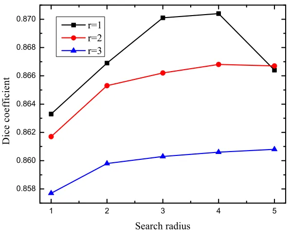
The proposed method has two parameters, r for the local patch radius and rs for

the local searched neighborhood. The influence of these parameters are studied by evaluating a range of values r∈ {1,2,3}; rs ∈ {1,2,3,4,5} in the experiment. First,

(52)

1 2 3 4 5 0.858 0.860 0.862 0.864 0.866 0.868 0.870 D i c e c o e f f i c i e n t Search radius r=1 r=2 r=3

Figure 3.2: Hippocampus segmentation performance using different patch radius and searched patch radius.

Dice coefficient decreases when the searched radius rs > 4. Larger searched radius

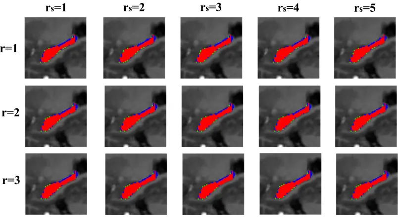
improves the probability to find a similar patch with target patch, however, it also leads to an increase of mismatches. Figure3.2 indicates that the best Dice coefficient is obtained atr = 1 andrs = 4. Figure3.3 shows the segmentation results for different

sizes of local patch and searched patch.

3.3.2 Comparison Results in Hippocampus Segmentation

(53)

Figure 3.3: Sagittal views of the segmentations produced by different patch radius and searched patch radius. Where the red region shows the overlap between the automatic and the manual segmentation; the green region is the manual segmentation; and the blue region is automatic segmentation using the proposed method.

(54)

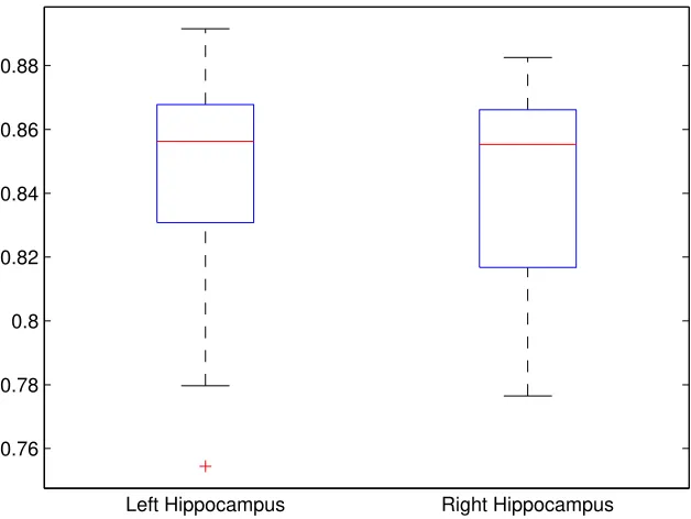
0.76 0.78 0.8 0.82 0.84 0.86 0.88

Left Hippocampus Right Hippocampus

Figure 3.4: The dice overlap coefficient of the left and right hippocampus

3.4 Discussion and Conclusion

(55)

Chapter 4 Supervoxel Based Method for

Multi-Atlas Segmentation of Brain

MR Images

(56)

4.1 Introduction

An alternative method for segmentation is to formulate it as the energy minimization associated with the graphical model, in which the atlases are used to provide the prior knowledge about the spatial constraints [107]. As a result, the graphical model is usually considered as a post-processing technique to refine the results of the multi-atlas label fusion [3, 64, 84].

However, as an important pre-processing step of multi-atlas segmentation, the pairwise registration plays a crucial role in learning the spatial prior information for the MAP inference methods. Both the label fusion method and energy minimization method heavily rely on the complicated pairwise registration. Although the patch-based technique is effective in accounting for the registration errors, the performance is affected by the search radius of the local neighborhood in the registered atlases [26]. Increasing the search radius will greatly increase the computational cost while using a small search radius is not effective enough to remedy the registration errors. To address these limitations, a graphical model-based multi-atlas segmentation algorithm from the supervoxel perspective is proposed. Superpixel-based MRF frame-work has been successfully applied to the semantic natural scene segmentation [104]. Inspired by [104], we extend it to the brain MR image segmentation using a su-pervoxel graphical model. The susu-pervoxel is an aggregation of voxels with similar attributes, and thus, we can assume that the voxels within the supervoxel have the same label. Based on this assumption, each node in the graphical model is associated with a supervoxel, and the label minimizing the energy function is thus assigned to each element voxel within the supervoxel.

(57)

a post-processing step, based on a grid graphical model with a high order potential, is performed to refine the supervoxel labeling results. The major contributions of this work include:

1. The spatial consistency is encouraged in the proposed method. According to the definition of supervoxel, the labels within the supervoxel are spatially consistent. In addition, the label consistency between neighboring supervoxels is encouraged by the smoothness term in the energy function.

2. The proposed method is robust to the pairwise registration errors. It searches similar atlas supervoxels in the neighborhood and encodes the supervoxel similarity into the data term of the energy function. It differs from the patch-based technique in that the search radius is defined by the number of supervoxels instead of voxels, which results in a larger search range given a fixed search radius. Consequently, the spatial prior is acquired by the initialization of the data term, rather than the sophisticated pairwise registration, and the dependency on the complicated pairwise registration is greatly alleviated.

3. The proposed approach is computationally efficient. Since the supervoxels are used as nodes in the graph construction, the number of nodes decreases to around 1/n of that in the voxel-based graphical models, where n is the average size of the supervoxels. Moreover, thanks to the insensitivity to the pairwise registration, affine registration can be used as a substitute for deformable registration so as to reduce the pre-processing time.

(58)

the advantages over the patch-based technique and learning-based methods are given in Section 4.4, and the paper is concluded in Section 4.5.

4.2 Method

Let IT be the target image IT = {IT(x)|x ∈ Ω}, where x denotes the voxel. The

goal of multi-atlas segmentation is to estimate a label map LT which assigns a label

lx ∈ {1, . . . ,L} to each voxel in the target image, given K atlases A1, . . . , AK with

Ak = (Ik, Lk) where Ik and Lk are the intensity image and the corresponding label

image, respectively. This problem can be solved via MAP estimation [91] ˆ

LT = arg max L

p(IT, LT;{Ik, Lk}) (4.1)

wherep(IT, LT;{Ik, Lk}) is the joint probability ofIT andLT given the atlases. MRF

optimization is often posed as the task of finding the label map LT that optimizes

the MAP problem. The problem corresponds to minimizing the following objective function, known as MRF energy, which is defined over an undirected graph including node set Ω and edge set E

E( ˆLT) =

X

x∈Ω

θx(lx) +

X

x,y∈E

θxy(lx, ly) (4.2)

where the node set is referred to as the voxels in the target image while the edge set consists of the undirected edges in the graph connecting pairwise nodes. The unary data term θx(lx) encodes the probability of observing label lx at voxel x while the

smoothness termθxy(lx, ly) measures the cost of assigninglxandly to two neighboring

voxels which are connected by the corresponding edge.

In supervoxel graph, the supervoxels are considered as the nodes, the energy function is thus defined as:

E( ˆLT) =

X

s∈Ωs

θs(ls) +

X

s,t∈Es

Brain MR Image Segmentation: From Multi-Atlas Method To Deep Learning Models

Scholarship at UWindsor

Scholarship at UWindsor

Brain MR Image Segmentation: From Multi-Atlas Method To Deep

Brain MR Image Segmentation: From Multi-Atlas Method To Deep

Learning Models

Learning Models

BRAIN MR IMAGE SEGMENTATION:

FROM MULTI-ATLAS METHOD TO DEEP LEARNING

MODELS

by

Jie Huo

BRAIN MR IMAGES SEGMENTATION:

FROM MULTI-ATLAS METHOD TO DEEP LEARNING

MODELS

Declaration of Co-Authorship / Previous

Publication

I Co-Authorship Declaration

II Previous Publication

III General

Abstract

Dedication

Acknowledgements

Table of Contents

List of Tables

List of Figures

List of abbreviation

Chapter 1

Introduction

1.1

Segmentation of Brain MR Images

1.2

Motivation

1.3

Challenges

1.4

Objective and Contributions

1.5

Organization of Thesis

Chapter 2

Background

2.1

Overview

2.2

Multi-atlases Segmentation

2.2.1

Background

2.2.2

Related Work

2.3

Random Field for Segmentation Problem

2.3.1

Background

2.3.2

Related Work

2.4

Convolutional Neural Network

2.4.1

Background

2.4.2

Related Work

2.5

MRI Coordinate System

2.6

Datasets

2.7

Image Pre-Processing

Chapter 3

Label Fusion for Multi-Atlas

Segmentation Based on Majority

Voting

3.1

Introduction

3.2

Method

3.2.1

Patch Selection

3.2.2

Label Fusion and Validation

3.3