Electronic Structure of Heavy Element Systems and Many-body Constructions of High-accuracy Effective Core Potentials.

(1)

Abstract

BENNETT, MICHAEL CHANDLER. Electronic Structure of Heavy Element Systems and Many-Body Constructions of High-Accuracy Effective Core Potentials. (Under the direction of Lubos Mitas).

The electronic structure of atomic, molecular, and solid state systems provides key

insights into their rich variety of properties. Fundamental to understanding the electronic

structure of these systems are the solutions to the time-independent Schrödinger equation

under the Born-Oppenheimer approximation. However, due to the inter-particle

interac-tions of the electrons, an exact polynomial scaling algorithm for solving the equation does not exist. As a result, a vigorous pursuit of simplifications and approximations, that keep

the predictive power of the equation intact, has been underway since the birth of quantum

theory in the 1920s. This pursuit, in tandem with exponentially increasing computational

power, has lead to the development of a number of high-accuracy methodologies. Of

par-ticular prominence, is the diffusion Monte Carlo method which benefits from low-order

polynomial-scaling, applicability over a wide range of system sizes – up to hundreds of

electrons, and a small number of fully specified errors.

We have applied diffusion Monte Carlo to various heavy transition metal systems. These

systems are attractive from a theoretical point of view due to the presence of localized

d-electrons which consequently results in significant amounts of correlation and therefore are challenging for electronic structure methods in general. We study trends in the errors of

diffusion Monte Carlo under the fixed-node approximation in order to better understand

the accuracy limits of the method for these systems in various environments. Additionally,

we investigate a specific error that is present within diffusion Monte Carlo studies of heavy

elements due to the unavoidable introduction of pseudopotentials. From coupled-cluster

calculations, we find that the errors of tabulated pseudopotentials within molecular settings

can be significant relative to all-electron results for high-accuracy many-body techniques

especially when the molecules are out of equilibrium configurations. We develop a strategy to generate pseudopotentials that incorporates near-exact correlated many-body spectra

and properties and as a result lead to high accuracy over a test bed of molecules – both

within and out of equilibrium. We use this strategy to develop pseudopotentials for 1st_row

(2)

(3)

Electronic Structure of Heavy Element Systems and Many-Body Constructions of High-Accuracy Effective Core Potentials

by

Michael Chandler Bennett

A dissertation submitted to the Graduate Faculty of North Carolina State University

in partial fulfillment of the requirements for the Degree of

Doctor of Philosophy

Physics

Raleigh, North Carolina

2019

APPROVED BY:

Jerzy Bernholc Alexander Kemper

Jerry Whitten Lubos Mitas

(4)

Dedication

Dedicated to my parents who made it possible

And to Cassidy who drove me to see it through

(5)

Biography

My interest for physics developed midway through my undergraduate studies. I was drawn

specifically to physics after reading popular physics literature out of mild curiosity. These

qualitative treatments of classical and modern theories proved to be unimaginably

seduc-tive. Instantly, I recognized the importance in humanity’s pursuit of a deeper understanding

of the universe. As a consequence I felt urged to play a part in this pursuit – I had to

con-tribute. At the time I had nearly fulfilled all requirements for a bachelor’s in computer science. Given that computation was, as it continues to be, an integral component of

nu-merous research topics in physics, I was confident that continuing to refine my skills in

programming while also inundating my academic schedule with courses in core areas of

physics would provide me with a unique set of talents which I could then apply to the

further discovery of new ideas in the field. After completing my undergraduate studies I was

accepted into NCSU’s Master of Computer Science program. During my second semester

there I enrolled in the first part of a two-part sequence of upper-level undergraduate

classi-cal mechanics (at the level of Marion). Upon completion of this course, my interest in the

subject was affirmed and I grew hungry for more. I continued to consume further topics in physics through coursework, while also continuing to complete the master’s

require-ments, and I began to acquire more specific interests in the field. As a consequence of

taking Dr. Lubos Mitas’ course in computational physics I developed an interest in the

study of nanoscience and materials physics. In this course, I recognized how beneficial the

marriage of theory and machine can be – the ability to extract unexpected properties and

new understanding of these systems from simulation were benefits I found exceptionally

satisfying not to mention beautiful. After graduating with my master’s, I was invited into

NCSU’s physics PhD program where I joined Professor Mitas’ research group enabling me

(6)

Acknowledgements

I am particularly grateful to my advisor, Professor Lubos Mitas. Throughout my PhD, he has

been supportive and encouraging while also cultivating an atmosphere that has driven me

to continually improve in all aspects of my work. His enthusiasm for science is contagious

and I have been lucky to have him as a mentor these last few years.

I am also grateful to Luke Shulenburger and Thomas Mattsson, who provided me with

the opportunity to take part in research within a laboratory setting during my PhD studies. This experience was vastly enriching and strengthened my abilities as a researcher. I greatly

appreciate the chance to work along side them.

I would also like to thank the current and past members of the Mitas group. Special

thanks to Adem Kulahlioglu and Kevin Rasch, each being particularly helpful mentors when

I first entered the group. I am also grateful for the many invaluable discussions with Cody

Melton and have enjoyed being colleagues during our time in the group.

Finally, I am tremendously thankful to all the love and support from my family and

(7)

List of Tables

Table 3.1 The structural parameters are given. The bond lengths (R/Å) and dihedral angles (∠/◦_{) were obtained from DFT-TPSSh calculations. . .} ₂₉

Table 3.2 Bond distances (R/Å) and dihedral angles (∠/◦_{) of WBz. . . .} ₃₁

Table 3.3 Bond distances (R/Å) and dihedral angles (∠/◦_{) of WBz}

2. . . 31 Table 3.4 Binding energies[eV]of W-Bz and W-Bz₂and systems from DFT

meth-ods and from fixed-node DMC with two trial wave functions con-structed with PBE and PBE0 orbitals. . . 32

Table 4.1 PbH bond length (re) and dissociation energy (De) . . . 62 Table 4.2 Excitation energies for the Sn atom from the3_P

0 ground state. We include both LC and SC PPs. For completeness, we include COSCI and FCI to compare the FPSODMC and experiment[Nis]. . . 63 Table 4.3 Electron Affinities for the 6p elements. COSCI trial wave functions

used throughout, with LC AREP/REPs for Pb[MS00], Bi[Sto02], Po[Sto02], and At[Sto02]. For Tl, no LC REP was found, so we utilize a SC AREP/REP [Met00]. . . 66 Table 5.1 Atomic and ionic excitations and corresponding discrepancies for

Boron. IP denotes the first ionization potential while EA is the electron affinity. Q is the ionization charge, 2S+1 the usual total spin multi-plicity. AE denotes the calculated all-electron values while the rest of columns shows the discrepancies. UC means all-electron valence-only correlation with self-consistent but uncorrelated core, as explained in the text. All energies in eV. The MAD is the mean absolute difference over all of the discrepancies. Note that all gaps are calculated with reference to the ground state, namely Q=0 and 2S+1=2. The same notation applies to all the atomic/ionic data tables throughout the paper. . . 79 Table 5.2 ECP parameters for Constructed Boron. The parametrization for each

channel is given byVl(r) =

P

kβl krnl k−2e−αl kr 2

. The corresponding correlation consistent basis sets are included in the Supplementary Material. . . 81 Table 5.3 Atomic data for Carbon, similar to Table 5.1. Energies in eV. Note that

all gaps are calculated with reference to the ground state, namely Q=0 and 2S+1=3. . . 83 Table 5.4 ECP parameters for Constructed Carbon. The parametrization for each

P

(12)

Table 5.5 Atomic data for Nitrogen, similar to Table 5.1. Energies in eV. Note that all gaps are calculated with reference to the ground state, namely Q=0 and 2S+1=4. . . 84 Table 5.6 ECP parameters for Constructed Nitrogen. The parametrization for

each channel is given byVl(r) =

P

. The correspond-ing correlation consistent basis sets are included in the Supplementary Material. . . 86 Table 5.7 Atomic data for Oxygen, similar to Table 5.1. Energies in eV. Note that

all gaps are calculated with reference to the ground state, namely Q=0 and 2S+1=3. . . 88 Table 5.8 ECP parameters for Spectral Oxygen. The parametrization for each

P

. The corresponding correlation consistent basis sets are included in the Supplementary Material. . . 88 Table 5.9 Atomic data for Sulfur, similar to Table 5.1. Energies in eV. Note that

all gaps are calculated with reference to the ground state, namely Q=0 and 2S+1=3. . . 89 Table 5.10 ECP parameters for Constructed ECP for Sulfur. The parametrization

for each channel is given byVl(r) =

P

. The corre-sponding correlation consistent basis sets are included in the Supple-mentary Material. . . 92 Table 5.11 Mean absolute deviations of discrepancies of binding parameters

at equilibrium (De,re andωe) and near the dissociation threshold (Dd i s s) at short bond lengths for our ECPs and previous constructions with respect to all-electron CCSD(T) calculations. The system sets correspond to Fig.5.14 except for the BH₃molecule which was omitted from the MADs of the dissociation threshold energy. . . 93

Table 6.1 Parameter values for Ne-core ECPs. For all ECPs, the highestl value corresponds to the local channel. . . 110 Table 6.2 Parameter values for He-core ECPs. For all ECPs, the highestl value

corresponds to the local channel. . . 111 Table 6.3 All-electron (AE) UCCSD(T) electron affinity and ionization potential

of Na along with the errors from uncorrelated core (UC), ECPs and for information purposes also from experiment (Exp.). The uncontracted aug-cc-pCV5Z basis was used for all calculations. MAD is the mean absolute deviation of excitation energies, while MARE is the mean absolute relative error. All values in eV. . . 114 Table 6.4 All-electron UCCSD(T) ionization potentials for Mg along with the

(13)

Table 6.5 All-electron (AE) UCCSD(T) ionization potentials and electron affinity of Al along with the errors from the uncorrelated core (UC) and ECPs. Exp. gives experimental values for information purposes. The uncon-tracted aug-cc-pCV5Z basis was used for all calculations. AMAD is the mean absolute deviation for all excitation energies, LMAD is the mean absolute deviation for the first and second ionization potentials and electron affinity, while MARE is the mean absolute relative error for all states. All values in eV. . . 117 Table 6.6 All-electron (AE) UCCSD(T) ionization potentials and electron affinity

of Si along with the errors from uncorrelated core (UC) and ECPs. The uncontracted aug-cc-pCV5Z basis was used for all calculations. All values in eV. See Tab. V for further description. . . 119 Table 6.7 All-electron (AE) UCCSD(T) ionization potentials and electron affinity

of P along with the errors from uncorrelated core (UC) and ECPs. The uncontracted aug-cc-pCV5Z basis was used for all calculations. All values in eV. See Tab. V for further description. . . 121 Table 6.8 All-electron (AE) UCCSD(T) valence ionization potentials and

elec-tron affinity of S along with the errors from uncorrelated core (UC) and ECPs. The uncontracted aug-cc-pCV5Z basis was used for all cal-culations. All values in eV. See Tab. V for further description. . . 123 Table 6.9 All-electron (AE) UCCSD(T) ionization potentials and electron affinity

of Cl along with the errors from uncorrelated core (UC) and ECPS. The uncontracted aug-cc-pCV5Z basis was used for all calculations. All values in eV. See Tab. V for further description. . . 125 Table 6.10 All-electron (AE) UCCSD(T) ionization potentials for Ar along with

the errors from uncorrelated core (UC) and ECPs. The uncontracted aug-cc-pCV5Z basis was used for all calculations. All values in eV. See Tab. V for further description. . . 127 Table 6.11 Mean absolute deviations of discrepancies of binding parameters

of all molecules considered in this work at equilibrium (De,re and

(14)

Table 6.12 Total energies of our ccECPs with Ne (LC) and He (SC) cores in their neutral ground states along with their core radii for each angular mo-mentum channel – the valuesrl are taken as the distance which the channel’s full potential agrees with the bare Coloumb potential to within 10−5_{Ha while}_r

l,nlis the distance at which the channel’s non-local potential drops below 10−5_{Ha. Both RHF}_/_{ROHF and UCCSD(T)} correlation energies are extrapolated to the CBS limit using the un-contracted aug-cc-pwCV{T,Q,5}Z bases. Energies given in Ha. Radii given in Å. . . 130

Table 7.1 A summary of the atomic state discrepancy data. For each atom, we provide mean absolute deviations (MADs). LMAD corresponds to the low-lying atomic spectrum, which includes the electron affinity, ion-ization potential, and the neutral and first ionizeds↔d transitions. The MAD includes the LMAD as well as ionizations down to the Ar core. A_∗indicates that the our final ccECP is equivalent to our spectral only ccECP.S, as described in the atomic sections. N/A indicates that the particular ECP does not exist. . . 147 Table 7.2 Parameter values for hydrogen. The highestl value corresponds to the

local channel. Each term takes the formV_`k(r) =β`krn`k−2exp

−α`kr2

163 Table 7.3 Mean absolute deviations of binding parameters for various core

ap-proximations with respect to AE data for transition metal hydride and oxide molecules. All parameters were obtained using Morse potential fit. The parameters shown are dissociation energyDe, equilibrium bond lengthre, vibrational frequencyωe and binding energy discrep-ancy at dissociation bond lengthDd i s s. . . 165 Table 7.4 Parameter values for early transition metal ECPs. For all ECPs, the

highestl value corresponds to the local channel. Each term takes the formV_`k(r) =β`krn`k−2exp

−α`kr2

. . . 166 Table 7.5 Parameter values for late transtion metal ECPs. For all ECPs, the

high-estl value corresponds to the local channel. Each term takes the form

V_`k(r) =β`krn`k−2exp

−α`kr2

. . . 166

Table 8.1 Total energies for WO for the3_Σ_and5_Π_{states at}_r

e =1.67 Å. These results only utilize a scalar relativistic Hamiltonian and neglects spin-orbit. . . 179 Table 8.2 FNDMC (AREP) and FPSODMC (REP) dissociation energies of W₂

(15)

Table A.1 The uncontracted aug-cc-pCV5Z basis set errors (a.u.) corresponding to nitrogen’s CCSD(T) excitation energies calculated in the main text. 203 Table A.2 The uncontracted aug-cc-pCV5Z basis set errors (a.u.) corresponding

to sulfur’s CCSD(T) excitation energies calculated in the main text. . . 204

Table A.3 Correlation Consistent basis sets for the Boron ECP . . . 205

Table A.4 Correlation Consistent basis sets for the Carbon ECP . . . 206

Table A.5 Correlation Consistent basis sets for the Nitrogen ECP . . . 207

Table A.6 Correlation consistent basis set for the Oxygen ECP. . . 208

Table A.7 Correlation Consistent basis sets for the Sulfur ECP . . . 209

Table B.1 Total energy components of various states of the Na atom using our ccECP[Ne] . . . 211

Table B.2 Total energy components of various states of the Na atom using our ccECP[He] . . . 211

Table B.3 Total energy components of various states of the Mg atom using our ccECP[Ne] . . . 211

Table B.4 Total energy components of various states of the Mg atom using our ccECP[He] . . . 212

Table B.5 Total energy components of various states of the Al atom using our ccECP[Ne] . . . 212

Table B.6 Total energy components of various states of the Al atom using our ccECP[He] . . . 213

Table B.7 Total energy components of various states of the Si atom using our ccECP[Ne] . . . 213

Table B.8 Total energy components of various states of the Si atom using our ccECP[He] . . . 214

Table B.9 Total energy components of various states of the P atom using our ccECP[Ne] . . . 214

Table B.10 Total energy components of various states of the P atom using our ccECP[He] . . . 215

Table B.11 Total energy components of various states of the S atom using our ccECP[Ne] . . . 215

Table B.12 Total energy components of various states of the S atom using our ccECP[He] . . . 216

Table B.13 Total energy components of various states of the Cl atom using our ccECP[Ne] . . . 217

Table B.14 Total energy components of various states of the Cl atom using our ccECP[He] . . . 218

Table B.15 Total energy components of various states of the Ar atom using our ccECP[Ne] . . . 219

(16)

Table B.17 All-electron (AE) UCCSD(T) Na2 ground state (1_Σ

g) binding parame-ters and potential energy surface along with the errors from uncorre-lated core (UC) and ECPs. All energies in eV. . . 221 Table B.18 All-electron (AE) UCCSD(T) NaO ground state (2Σ) binding

parame-ters and potential energy surface along with the errors from uncorre-lated core (UC) and ECPs. All energies in eV. . . 222 Table B.19 All-electron (AE) UCCSD(T) MgO ground state (1Σ+) binding

parame-ters and potential energy surface along with the errors from uncorre-lated core (UC) and ECPs. All energies in eV. . . 222 Table B.20 All-electron (AE) UCCSD(T) Al2 ground state (3Σg) binding parameters

and potential energy surface along with the errors from uncorrelated core (UC) and ECPs. All energies in eV. . . 224 Table B.21 All-electron (AE) UCCSD(T) AlO ground state (2Σ) binding parameters

and potential energy surface along with the errors from uncorrelated core (UC) and ECPs. All energies in eV. . . 224 Table B.22 All-electron (AE) UCCSD(T) Si2 ground state (3Σg) binding parameters

and potential energy surface along with the errors from uncorrelated core (UC) and ECPs. All energies in eV. . . 225 Table B.23 All-electron (AE) UCCSD(T) SiO ground state (1Σ) binding parameters

and potential energy surface along with the errors from uncorrelated core (UC) and ECPs. All energies in eV. . . 225 Table B.24 All-electron (AE) UCCSD(T) P2 ground state (1Σg) binding parameters

and potential energy surface along with the errors from uncorrelated core (UC) and ECPs. All energies in eV. . . 226 Table B.25 All-electron (AE) UCCSD(T) PO ground state (2Π) binding parameters

and potential energy surface along with the errors from uncorrelated core (UC) and ECPs. All energies in eV. . . 226 Table B.26 All-electron (AE) UCCSD(T) S2 ground state (3Σg) binding parameters

and potential energy surface along with the errors from uncorrelated core (UC) and ECPs. All energies in eV. . . 227 Table B.27 All-electron (AE) UCCSD(T) SO ground state (3Σ) binding parameters

and potential energy surface along with the errors from uncorrelated core (UC) and ECPs. All energies in eV. . . 227 Table B.28 All-electron (AE) UCCSD(T) Cl2 ground state (1Σg) binding

parame-ters and potential energy surface along with the errors from uncorre-lated core (UC) and ECPS. All energies in eV. . . 228 Table B.29 All-electron (AE) UCCSD(T) ClO ground state (2Π) binding parameters

(17)

Table B.30 All-electron (AE) UCCSD(T) ArH+ground state (1_Σ_{) binding} parame-ters and potential energy surface along with the errors from uncorre-lated core (UC) and ECPs. All energies in eV. . . 229 Table B.31 Parameter values for Cl and Ar ccECP[Ne].S potentials. The highestl

value corresponds to the local channel. . . 229 Table B.32 All-electron (AE) UCCSD(T) ionization potentials and electron affinity

of Cl along with the errors from ccECP[Ne].S. The uncontracted aug-cc-pCV5Z basis was used for all calculations. All values in eV. See Tab. V in main text for further description. . . 230 Table B.33 All-electron (AE) UCCSD(T) Cl2 ground state (1Σg) binding

parame-ters and potential energy surface along with the errors from ccECP[Ne].S. All energies in eV. . . 230 Table B.34 All-electron (AE) UCCSD(T) ClO ground state (2Π) binding parameters

and potential energy surface along with the errors from ccECP[Ne].S. All energies in eV. . . 231 Table B.35 All-electron (AE) UCCSD(T) ionization potentials and electron affinity

of Ar along with the errors from ccECP[Ne].S. The uncontracted aug-cc-pCV5Z basis was used for all calculations. All values in eV. See Tab. V in main text for further description. . . 231 Table B.36 All-electron (AE) UCCSD(T) ArH+ground state (1_Σ_{) binding}

parame-ters and potential energy surface along with the errors from ccECP[Ne].S. All energies in eV. . . 232

Table C.1 Total energy components of the[Ar]3d1₄_s2 2_D _{ground state of the Sc} atom using our ccECP. . . 235 Table C.2 Sc AE gaps and relative errors for various core approximations. All

gaps are relative to the[Ar]3d1₄_s2 2_D _{state. All values in eV. . . 235} Table C.3 ScH AE molecular binding parameters and discrepancies for

vari-ous core approximations. All parameters were obtained using Morse potential fit. The parameters shown are dissociation energyDe, equi-librium bond lengthre, vibrational frequencyωe and dissociation energy discrepancy at dissociation bond lengthDd i s s. . . 236 Table C.4 ScO AE molecular binding parameters and discrepancies for various

core approximations. Labeling as in Table C.3 . . . 236 Table C.5 Total energy components of the[Ar]3d2₄_s2 3_F _{ground state of the Ti}

atom using our ccECP. . . 237 Table C.6 Ti AE gaps and relative errors for various core approximations. All in eV.237 Table C.7 TiH AE molecular binding parameters and discrepancies for various

core approximations. Labeling as in Table C.3 . . . 238 Table C.8 TiO AE molecular binding parameters and discrepancies for various

(18)

Table C.9 Total energy components of the[Ar]3d3₄_s2 4_F _{ground state of the V} atom using our ccECP. . . 238 Table C.10 V AE gaps and relative errors for various core approximations. All data

in eV. . . 239 Table C.11 VH AE molecular binding parameters and discrepancies for various

core approximations. Labeling as in Table C.3 . . . 239 Table C.12 VO AE molecular binding parameters and discrepancies for various

core approximations. Labeling as in Table C.3 . . . 240 Table C.13 Total energy components of the[Ar]3d5₄_s1 7_S_{ground state of the Cr}

atom for our ccECP. . . 240 Table C.14 Cr AE gaps and relative errors for various ECPs. All values in eV . . . 241 Table C.15 CrH AE molecular binding parameters and discrepancies for various

core approximations. Labeling as in Table C.3 . . . 241 Table C.16 CrO AE molecular binding parameters and discrepancies for various

core approximations. Labeling as in Table C.3 . . . 242 Table C.17 Total energy components of the[Ar]3d5₄_s2 6_S _{ground state of the Mn}

atom for our ccECP. . . 242 Table C.18 Mn AE gaps and relative error for various core approximations. All in eV.243 Table C.19 MnH AE molecular binding parameters and discrepancies for various

core approximations. Labeling as in Table C.3 . . . 243 Table C.20 MnO AE molecular binding parameters and discrepancies for various

core approximations. Labeling as in Table C.3 . . . 244 Table C.21 Total energy components of the[Ar]3d6₄_s2 5_D _{ground state of the Fe}

atom. . . 244 Table C.22 Fe AE gaps and relative errors for various ECPs. All data in eV . . . 245 Table C.23 FeH AE molecular binding parameters and discrepancies for various

core approximations. Labeling as in Table C.3 . . . 245 Table C.24 FeO AE molecular binding parameters and discrepancies for various

core approximations. Labeling as in Table C.3 . . . 246 Table C.25 Total energy components of the[Ar]3d7₄_s2 4_F _{ground state of the Co}

atom using our ccECP. . . 246 Table C.26 Co AE gaps and relative errors in eV . . . 246 Table C.27 CoH AE molecular binding parameters and discrepancies for various

core approximations. Labeling as in Table C.3 . . . 247 Table C.28 CoO AE molecular binding parameters and discrepancies for various

core approximations. Labeling as in Table C.3 . . . 247 Table C.29 Total energy components for the[Ar]3d8₄_s2 3_F _{state of the Ni atom}

for our ccECP. . . 248 Table C.30 Ni AE gaps and relative errors for various ECPs. All values in eV . . . 248 Table C.31 NiH AE molecular binding parameters and discrepancies for various

(19)

Table C.32 NiO AE molecular binding parameters and discrepancies for various core approximations. Labeling as in Table C.3 . . . 249 Table C.33 Total energy components of the[Ar]3d10₄_s1 2_S_{ground state of the Cu}

atom using our ccECP. . . 250 Table C.34 Cu AE and relative errors for various core approximations. All values

in eV . . . 250 Table C.35 CuH AE molecular binding parameters and discrepancies for various

core approximations. Labeling as in Table C.3 . . . 251 Table C.36 CuO AE molecular binding parameters and discrepancies for various

core approximations. Labeling as in Table C.3 . . . 251 Table C.37 Total energy components for the[Ar]3d10₄_s2 1_S _{ground state of the}

Zn atom using our ccECP. . . 252 Table C.38 Zn AE gaps and relative errors for various ECPs. All values in eV . . . . 252 Table C.39 ZnH AE molecular binding parameters and discrepancies for various

core approximations. Labeling as in Table C.3 . . . 253 Table C.40 ZnO AE molecular binding parameters and discrepancies for various

(20)

List of Figures

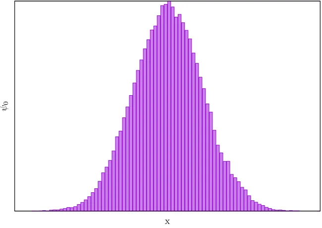
Figure 2.1 A diffusion Monte Carlo simulation of the ground state of a one-dimensional harmonic oscillator. The walkers are initially distributed uniformly then evolved through 8 units of imaginary time and the birth/death re-weighting scheme is used during their evolution. After the simulation completes, the walkers are distributed according to ψ0as expected. . . 20

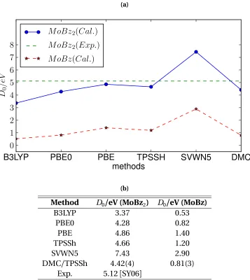
Figure 3.1 Molecular geometries of (a) bis(benzene)molybdenum (MoBz₂) and (b) mono(benzene)molybdenum (MoBz). The geometries of the cor-responding W systems are similar. . . 27 Figure 3.2 The binding energies of the MoBz₂and MoBz molecules calculated

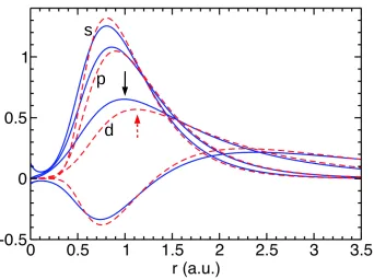
by DFT and FNDMC methods compared with experiment (a) and (b). FNDMC trial function has been constructed using TPSSh functional. 30 Figure 3.3 Radial components ofs(`=0),p(`=1)andd(`=2)valence

pseu-dorbitals plotted asr`%_`(r)for Mo (full, blue) and W (dashed, red) atoms. The maximum ofs-orbital for W is higher than for Mo (rel-ativity), while the opposite is true in thed−channel. Also note the significantly larger radius of the maximum (indicated by arrows) with the consequent smaller amount of charge in the core region in the

d−channel of W. . . 33

Figure 4.1 Total Energy of the Pb ground state. The “No Drift” and “Drift” calcu-lations are indistinguishable at this scale. . . 57 Figure 4.2 Total energies of the Pb ground state with COSCI trial wave functions.

The calculations were performed with drift,vS

D 6=0, and excluding drift,vS

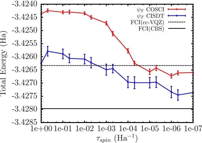
D=0. . . 59 Figure 4.3 Total energy using COSCI and CISDT trial wave functions for the Pb

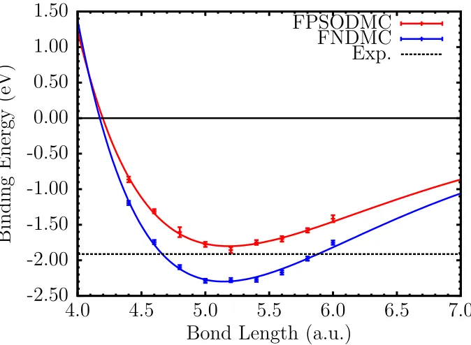
ground state. FCI with cc-VQZ and a CBS extrapolation are included as a reference. . . 60 Figure 4.4 Binding Curve of the Sn₂molecule using averaged spin-orbit AREP

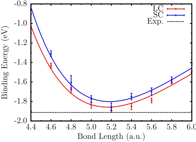
with FNDMC and spin-orbit REP with FPSODMC methods. The curves are offset to dissociation limit 2E0(Sn)within each method to enable comparison for the predicted binding energy of each method with experiment. . . 64 Figure 4.5 Binding curve of the Sn2molecule using large- and small-core REP.

(21)

Figure 5.1 Boron dimer potential energy surface. UC represents an all-electron CCSD(T) calculation with a self-consistent butuncorrelatedcore, i.e., with no excitations from the core states. Spectral represents the opti-mization for the atomic spectrum alone, and Constructed indicates the ECP driven iteratively to minimize the dimer discrepancy while accepting a small increase in the spectrum discrepancy. . . 80 Figure 5.2 Boron dimer binding energy discrepancies compared to the all-electron

CCSD(T) binding curve. The gray envelope represents a 0.05 eV win-dow for the discrepancy. The vertical line indicates the equilibrium bond length as predicted by the all-electron CCSD(T) calculation. . 81 Figure 5.3 Carbon dimer binding energy discrepancies compared to the

all-electron CCSD(T) binding curve. . . 83 Figure 5.4 Nitrogen dimer binding energy discrepancies compared to the

all-electron CCSD(T) binding curve. . . 85 Figure 5.5 Oxygen dimer binding energy discrepancies compared to the

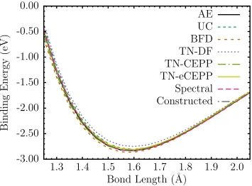
all-electron CCSD(T) binding curve. . . 87 Figure 5.6 Potential energy surfaces of the S₂molecule from CCSD(T). We have

plotted the predictions from various treatments of the sulfur cores. Shown are the all-electron core (AE), all-electron uncorrelated core (UC), Burkatzki-Filippi-Dolg (BFD), Dirac-Fock Trail-Needs (TN) and the CCSD(T) spectrum matched (Spectral) ECPs described in the text. 89 Figure 5.7 Sulfur dimer binding energy discrepancies compared to the all-electron

CCSD(T) binding curve. . . 90 Figure 5.8 Sulfur dimer binding energy discrepancies compared to the all-electron

CCSD(T) binding curve. . . 91 Figure 5.9 NH binding energy discrepancies for various ECPs . . . 94 Figure 5.10 OH binding energy discrepancies for various ECPs. For Oxygen, we

use our spectral ECP. . . 95 Figure 5.11 NO binding energy discrepancies for various ECPs. For Nitrogen, we

use our constructed ECP and for Oxygen, we use our spectral ECP. . . 96 Figure 5.12 SH binding energy discrepancies compared to the all-electron CCSD(T)

binding curve. For Sulfur, we use our constructed ECP and for Oxygen, we use our spectral ECP. . . 97 Figure 5.13 SO binding energy discrepancies compared to the all-electron CCSD(T)

binding curve. For Sulfur, we use our constructed ECP. . . 98 Figure 5.14 Discrepancies of molecular binding parameters of our ECPs, UC and

(22)

Figure 6.1 For the silicon atom, the spread of CCSD(T) valence-valence cor-relation errors (∆cVV) and spread of HF errors (∆HF) for various excitation energies from a variety of previously tabulated ECPs, in particular, BFD[Bur07], CRENBL[PC85], SBKJC[Ste84], STU[Dol87] and TN-DF[TN05]. . . 105 Figure 6.2 For the phosphorus atom, the spread of CCSD(T) valence-valence

correlation errors (∆cVV) and spread of HF errors (∆HF) for various excitation energies from a variety of previously tabulated ECPs, in particular, BFD[Bur07], CRENBL[PC85], SBKJC[Ste84], STU[Dol87] and TN-DF[TN05]. . . 106 Figure 6.3 Binding energy discrepancies for (a) Na₂ and (b) NaO molecules

in their ground states1_Σ

g and2Σ, respectively. The binding curves are relative to the AE UCCSD(T) binding curve. The shaded region indicates a discrepancy of chemical accuracy in either direction. . . . 115 Figure 6.4 Binding energy discrepancies for the MgO molecule in its ground

state1Σ+. The binding curves are relative to the AE UCCSD(T) bind-ing curve. The shaded region indicates a discrepancy of chemical accuracy in either direction. . . 116 Figure 6.5 Binding energy discrepancies for (a) Al2 and (b) AlO molecules in their

ground states3_Σ

g and2Σ, respectively. The binding curves are relative to the AE UCCSD(T) binding curve. The shaded region indicates a discrepancy of chemical accuracy in either direction. . . 118 Figure 6.6 Binding energy discrepancies for (a) Si2 and (b) SiO molecules in their

ground states3_Σ

g and1Σ, respectively. The binding curves are relative to the AE UCCSD(T) binding curve. The shaded region indicates a discrepancy of chemical accuracy in either direction. . . 120 Figure 6.7 Binding energy discrepancies for (a) P2 and (b) PO molecules in their

ground states1Σgand2Π, respectively. The binding curves are relative to the AE UCCSD(T) binding curve. The shaded region indicates a discrepancy of chemical accuracy in either direction. . . 122 Figure 6.8 Binding energy discrepancies for (a) S2and (b) SO molecules in their

ground states3_Σ

g and3Σ, respectively. The binding curves are relative to the AE UCCSD(T) binding curve. The shaded region indicates a discrepancy of chemical accuracy in either direction. . . 124 Figure 6.9 Binding energy discrepancies for (a) Cl2 and (b) ClO molecules in

their ground states1_Σ

(23)

Figure 6.10 Binding energy discrepancies for the ArH+molecule in its ground state1_Σ_{. The binding curves are relative to the AE UCCSD(T)} bind-ing curve. The shaded region indicates a discrepancy of chemical accuracy in either direction. . . 128

Figure 7.1 Spread of the contributions to the excitation energy for a variety of ECPs compared to all-electron for the Fe atom.∆HF shows the variation in the HF errors, whereas∆cVV shows the variation in the correlation energy error compared against the AE valence-valence correlation energy. . . 138 Figure 7.2 Discrepancies for the various core approximations compared to

all-electron CCSD(T) for select states. Each state discrepancy uses the neutrals2_dn_{occupation as the reference, which is the neutral ground} state for each transition metal except for Cr and Cu, which haves1_d5 and s1_d10 _{ground states correspondingly. (a) the neutral} _s2_dn _→ s1_dn+1_{excitation. (b) the neutral}_s2_dn_→_dn+2_{(c) the ionization from}

s2_dn _→_s1_dn _{(d) the ionization from}_s2_dn _→_[_Ar_]_{. The shaded gray} window in each figure indicates a discrepancy of half of chemical accuracy in either direction from the all-electron reference. We note that for Sc and Ti, our final ccECP is equivalent to our spectral ccECP.S.143 Figure 7.3 Mean Absolute Deviation, or MAD, for the TMs considering a large

part of the spectrum from[Ar]up to low-lying neutral excited states and the anion. The shaded region of half of chemical accuracy is not visible on this scale. We note that for Sc and Ti, our final ccECP is equivalent to our spectral ccECP.S . . . 144 Figure 7.4 Binding energy discrepancies for (a) ScH and (b) ScO molecules. The

binding curves are relative to the AE CCSD(T) binding curve. The shaded region indicates a discrepancy of chemical accuracy in either direction. . . 149 Figure 7.5 Binding energy discrepancies for (a) TiH and (b) TiO molecules. The

binding curves are relative to the CCSD(T) binding curve. The shaded region indicates a discrepancy of chemical accuracy in either direction.151 Figure 7.6 Binding energy discrepancies for (a) VH and (b) VO molecules. The

binding curves are relative to the CCSD(T) binding curve. The shaded region indicates a discrepancy of chemical accuracy in either direction.153 Figure 7.7 Binding energy discrepancies for (a) CrH and (b) CrO molecules. The

binding curves are relative to the CCSD(T) binding curve. The shaded region indicates a discrepancy of chemical accuracy in either direction.154 Figure 7.8 Binding energy discrepancies for (a) MnH and (b) MnO molecules.

(24)

Figure 7.9 Binding energy discrepancies for (a) FeH and (b) FeO molecules. The binding curves are relative to the CCSD(T) binding curve. The shaded region indicates a discrepancy of chemical accuracy in either direction.158 Figure 7.10 Binding energy discrepancies for (a) CoH and (b) CoO molecules.

The binding curves are relative to the CCSD(T) binding curve. The shaded region indicates a discrepancy of chemical accuracy in either direction. . . 159 Figure 7.11 Binding energy discrepancies for (a) NiH and (b) NiO molecules. The

binding curves are relative to the CCSD(T) binding curve. The shaded region indicates a discrepancy of chemical accuracy in either direction.161 Figure 7.12 Binding energy discrepancies for (a) CuH and (b) CuO molecules.

The binding curves are relative to the CCSD(T) binding curve. The shaded region indicates a discrepancy of chemical accuracy in either direction. . . 162 Figure 7.13 Binding energy discrepancies for (a) ZnH and (b) ZnO molecules.

The binding curves are relative to the CCSD(T) binding curve. The shaded region indicates a discrepancy of chemical accuracy in either direction. . . 164

Figure 8.1 FPSODMC total energies of WO molecule as a function of spin time stepτ_s/effective spin massµ_s for the lowest states with3_Σ_and5_Π symmetries. Note that the within the error bars the difference be-tween the states remains very similar regardless of the time step. . . . 180 Figure 8.2 The difference in the charge density between DHF and PBE0 trial

wave functions for the outermost spinorsπ4_σ2

z2σ2_sδ4. In red, we show where PBE0 has a greater charge density and in blue where DHF shows a greater charge density. The black spheres indicate the loca-tion of the Tungsten atoms. . . 182

Figure B.1 Binding energy discrepancies for (a) Cl2 and (b) ClO molecules in their ground states1_Σ

g and2Π, respectively. The binding curves are relative to the AE UCCSD(T) binding curve. The shaded region indi-cates a discrepancy of chemical accuracy in either direction. . . 223 Figure B.2 Binding energy discrepancies for the ArH+molecule in its ground

(25)

CHAPTER

1

Introduction

Quantum theory provides a remarkably accurate way to describe the properties of chemical

systems and materials. In fact, it was immediately clear after its birth in the early 20th_century

that quantum theory underpins the entire field of chemistry[DF29]and as a consequence precisely describes any system composed of either atoms, molecules, or both. This was an

astonishing success and the theory’s discovery represented a significant advancement in

humanity’s understanding of the Universe – this is evident if one considers the rich variety

of objects that exist above atomic scales and below scales relevant to the theory of gravity. As a practical matter, the human endeavour to improve technology drives the discovery of

new materials and their properties; with quantum theory in place, a complete description

of everyday material objects (both realized and unrealized) was available, for example,

reaction pathways of chemical substances, phase diagrams of materials, the hardness,

color, conductivity, and transparency of objects, and so on.

In the absence of time-varying external fields, the properties of these systems are

gov-erned primarily by the time-independent Schrödinger equation involving the constituent

electrons and nuclei. Solutions to this equation provide access to zero temperature and

finite-temperature properties and, in addition, time-independent and time-dependent phenomena. In practice, however, there is an impediment to utilizing the Schrödinger

(26)

polynomial-scaling solution to the equation so far does not exist. The difficulty stems from

the fact that for a quantum system of any practical interest, the number of composite

particles will be large – on the order of 1023_{for objects of human-scale volumes – and they}

undergo complicated motions due to pairwise interactions that depend on inter-particle

distances. This quantum many-body problem, as it is commonly referred, does not imply a

complete impasse, however. There has been much effort over many decades to construct

methodologies that provide solutions that are accurate enough for practical importance.

In the following section, an explicit description of the problem will be written down and

described. The subsequent sections will detail numerous methodologies that have been

formulated to yield approximate solutions to the quantum many-body problem involving electrons and nuclei – each with varying levels of sophistication and accuracy.

1.1 Electronic Structure

Throughout, atomic units (a.u.) will be used whereme =e =ħh =4πε0=1. In a.u., the time-independent Schrödinger for a general system ofN electrons andM nuclei, is given by  − 1 2 N X

i=1

∇2ri− 1 2

M

X

I=1 1

MI ∇2RI−

N

X

i=1 M

X

I=1

ZI |r_i₋R_I_|+

N

X

i<j 1

|r_i₋r_j_|+

M

X

I<J

ZIZJ |R_I₋R_J_|



Ψ=EΨ, (1.1)

where_{r_i_}and_{R_I_}are the sets of electron and nuclear positions, respectively, and_{MI}and {ZI}are the sets of nuclear masses and charges, respectively. Even for the lightest element, H, whose nucleus consists of just a single proton, the nuclear mass is nearly 2000 times

larger than the mass of the electron. To good approximation, therefore, the nuclei can be

assumed fixed in space and their respective kinetic energies can be dropped from equation

1.1 – this simplification is commonly known as the Born-Oppenheimer approximation.

Additionally, given that the nuclei are assumed fixed, the last term on the left-hand side of equation 1.1 is just a constant which can be removed then added back later if needed,

e.g., if a nuclear potential energy surface or cohesive energy, etc., is being calculated. Thus,

(27)

Schrödinger equation,



− 1 2

N

X

i=1

∇2ri−

N

X

i=1 M

X

I=1

ZI |r_i₋R_I_|+

N

X

i<j 1

|r_i₋r_j_|



Ψ=EΨ, (1.2)

which consists of the kinetic energy of the electrons, their interactions with the nuclei, and

their interactions with each other.

The field of electronic structure is devoted to using equation 1.2 to determine properties

of systems in atomic, molecular, or condensed phases. As a result, in fits and starts,

numer-ous methodologies have been developed to approximate solutions to the equation in an

attempt to reach levels of accuracy that are high enough such that quantitative predictions of these syatems can be made.

1.2 Hartree-Fock

The simplest way to avoid the difficulty of solving the electronic Schrödinger equation in the

presence of electron-electron interactions is to utilize the variational principle of quantum

mechanics and assume a trial wave function that is a product state of single-body orbitals.

This particular trial state is known as a Hartree product and neglects the interaction of the electrons as if the Hamiltonian were separable. The variational principle, for a trial state

|ΨT〉, asserts that the energy expectation value of|ΨT〉is no less than the exact ground state energy of the system, namely,

E0≤

〈ΨT|H|ΨT〉 〈ΨT|ΨT〉

(1.3)

whereH is the system’s Hamiltonian andE0is the ground-state eigenvalue ofH. SinceE0is the system’s ground state energy, that is, it is the lowest energy the system can possibly have,

it is then clear that equation 1.3 holds since in general_|ΨT〉is a superposition of eigenstates

ofH and its energy expectation value must be larger thanE0due to contributions from higher energy states.

For a system ofN electrons with space-spin coordinates{xi = (ri,ωi)}, the Hartree product wave function,〈X|ΨH〉, is given by

(28)

whereX≡(x1,x2, . . . ,xN)T are the combined coordinates of all the particles and{χi}is a set of one-particle spin-orbitals. Assuming that the orbitals are orthonormal, the energy

expectation value of the Hartree-product is

〈ΨH|H|ΨH〉= N

X

i=1 Z

d4xχ_i∗(x)

−1

2∇ 2₊_V

ions

χi(x)

+1

2 N

X

i=1 N

X

j6=i

Z d4x

Z d4x0

χ_i(x)

2 χ_j(x0)

2

|r₋r0_| . (1.5)

The optimum set of spin-orbitals can be derived by using the method of Lagrange

multipli-ers to minimize〈ΨH|H|ΨH〉with the constraint that the orbitals remain normalized

δ

〈ΨH|H|ΨH〉 − N

X

i=1 εi χi χ_i −1 ! =0 =⇒ N X

i=1 Z

d4xδχ_i∗(x)

(

−1

2∇ 2₊

Vions+ N

X

j6=i

Z d4x0

χ_j(x0)

2

|r₋r0_| −εi

) χi(x)

+complex conjugate=0 .

(1.6)

Since the variations ofδχ∗

i andδχiare independent and arbitrary, the expression in the curly brackets must be zero, which yields the following expression



− 1 2∇

2₊_V ions+

N

X

j6=i

Z d4x0

χ_j(x0)

2

|r−r0_|



χ_i(x) =ε_iχ_i(x). (1.7)

The set of equations defined by 1.7 are known as the Hartree equations. These equations are non-linear given that the potential (or field) felt by an electron in spin-orbitalχ_idepends

on the spin-orbitals of the other electrons and therefore the equations need to be solved in

an iterative fashion. The particular iterative process to solve the equations is known as the

self-consistent field (SCF) method in which a set of spin-orbitals is initially assumed and

used to define the field felt by each electron then the equations are solved for a new set of

spin-orbitals which are subsequently plugged back into the equations and solved again;

this process is iterated until the input and output spin-orbitals are identical to within some

tolerance (typically measured by the density, energy, or both).

(29)

electrostatics of the electrons and neglecting that they are indistinguishable particles which

should obey the Pauli exclusion principle. For identical fermions, the exclusion principle is

satisfied by wave functions that are antisymmetric under exchange of any pair of particle

coordinates,

Ψ(. . . ,xj, . . . ,xi, . . .) =−Ψ(. . . ,xi, . . . ,xj, . . .). (1.8)

An extension of the Hartree product that respects antisymmetry is the Slater determinant

which is defined as

Ψ(X) =_p1

N!

χ1(x1) χ2(x1) · · · χN(x1) χ1(x2) χ2(x2) · · · χN(x2)

..

. ... ...

χ1(xN) χ2(xN) · · · χN(xN)

, (1.9)

where 1/pN! is a normalization factor. The matrix here, with rows formed from particle coordinates and columns formed from spin-orbitals, is commonly referred to as the Slater

matrix. The antisymmetry of the Slater determinant follows from the property that inter-changing any two rows of a matrix changes the sign of its determinant and interinter-changing

two rows within a Slater matrix is equivalent to interchanging the coordinates of a pair of

particles.

If we minimize the energy expectation value of the Slater determinant with respect to

its spin-orbitals, as we did for the Hartree product, we arrive at the following equations for

the spin-orbitals  − 1 2∇ 2₊

Vions+ N

X

j=1 Z

d4x0

χ_j(x0)

2

|r₋r0_| − N

X

j=1 Z

d4x0

χ_j(x0)

2

|r₋r0_|

χj(x)

χj(x0)

χi(x0)

χi(x)



χ_i(x) =ε_iχ_i(x),

(1.10) which are the well-known Hartree-Fock equations. Notice the form here is consistent with

our assumption that the electrons occupy one-body spin-orbitals, that is, each electron

experiences an average potential, or mean-field, generated from the other electrons rather

than a (non-separable) pointwise interaction. This mean-field has two contributions; one

coming from pure electrostatics of the one-body densities as can be seen in the 3rd_{term in}

the square brackets of equation 1.10 and the other contribution is the exchange interaction,

(30)

the coordinates of the two particles as seen in the 4th_{term in the square brackets of equation}

1.10.

Relative to its simplicity, the accuracy of the Hartree-Fock wave function, – i.e., a Slater

determinant of Hartree-Fock orbitals – is quite high. For a general system, the energy

expectation value of this wave function is around 99% of the system’s exact ground state

energy. However, before we tempt ourselves into thinking that this accuracy will be good

enough for all practical purposes, consider how this picture can change when calculating an

energy difference. As an example, Hartree-Fock underbinds the carbon dimer significantly

and gives a binding energy,Eb =2E(C)−E(C2), that is only 8%-10% of the experimental value for this quantity. With a potential for errors as large as these, it is clear that the missing energy of Hartree-Fock, known as the correlation energy, can be critical for achieving useful

predictions for present (and future) experimental measurements.

1.3 Configuration Interaction

To capture the correlation energy missing from Hartree-Fock, a number of

post-Hartree-Fock methods have been formulated. One such method, known as configuration interaction

(CI), diagonalizes the Hamiltonian of the system in a many-body basis of Slater determi-nants. InfullCI, the basis is constructed by taking a set of single-body orbitals (generally

more thanN) then forming a basis of determinants from all possibleN-orbital combi-nations. Full CI gives an exact solution within the Hilbert space spanned by the set of

determinants and the set spans the full Hilbert space if the single-body orbitals span the

entire one-body Hilbert space. To see this, let us write down the expansion of an arbitrary

function of the coordinates of a single particle into a set of spin-orbitals

f (x) =X

i

aiχi(x). (1.11)

To form an arbitrary function,g, of the coordinates of two particles, we could then write

g(x,x0) =X

i

(31)

where we can then expand each function in the set_{aix0}into spin-orbitals, yielding

g(x,x0) =X

i

X

j

bi jχj(x0)χi(x). (1.13)

We can further impose thatg be antisymmetric and normalized,

g(x,x0) =_p1

2 X

i

X

j bi j

χj(x0)χi(x)−χi(x0)χj(x)

. (1.14)

Therefore, within the space spanned by_{χi}, an arbitrary antisymmetric function of the

coordinates of two particles is an expansion of Slater determinants formed from all combi-nations of spin-orbital pairs. For antisymmetric functions of the coordinates ofN particles, the same holds except the Slater determinants are formed from allN spin-orbital combina-tions.

Full CI, is not a feasible approach in practice given that the number of determinants

grows exponentially with the number of spin-orbitals. To combat this exponential blow-up,

various strategies truncate the number of determinants in some fashion. For instance, CI

with single and double excitations (CISD) uses all determinants formed from single- and

double-orbital excitations out of a Hartree-Fock reference determinant. Similarly, CISDT,

extends this to include triple-orbital excitations. One can push this as far as possible, i.e.,

CISDTQ, and so on, where each successive order obtains more and more of the correlation energy and therefore provides a systematically improvable approach.

Additionally, the multi-configurational self consistent field (MCSCF) approach goes a

step further and optimizes the spin-orbitals along with the CI expansion coefficients for a

given level of excitation. This can be achieved by first diagonalizing the Hamiltonian of the

system with a basis of determinants set by the chosen excitation level then constructing

natural orbitalsfrom this wave function – orbitals that diagonalize its single-body reduced

density matrix – then performing an additional diagonalization with the new set of orbitals.

The truncation schemes mentioned so far can often lead to qualitatively incorrect results

unless a high level of excitation can be chosen and therefore are not appropriate for larger systems. In addition, these methods suffer from a size consistency problem, that is when

calculating the energy of a system of constituent parts where the parts do not interact with

one another, the energy obtained is not equal to the sum of the energies obtained from

(32)

meaning they do not scale correctly for a system of interacting subsystems as the number

of subsystems is increased and therefore are infeasible to use for systems in the solid state.

Another truncation scheme, known as selected-CI, begins with a Hartree-Fock reference

and iteratively expands into larger numbers of determinants. At each round, the choice

of whether a determinant is included in the expansion is based on some criteria. This

approach attempts to build an expansion of themost importantdeterminants and is often

quite successful for small to medium sized systems.

1.4 Coupled Cluster

Similar in spirit to configuration interaction, is the coupled cluster method. In this approach,

an exponential ansatz is introduced

|ΨC C〉=eT|Ψ0〉 (1.15)

where

T =

N

X

i

Ti (1.16)

and each operator,Ti, generates a linear combination of all determinants which excitei electrons into the virtual (unoccupied) orbitals. In practice, a truncation scheme has to be

used here as well. One particular approach that is often used is to truncateT at double excitations, namelyT =T1+T2, then treat the triple excitations in a perturbative manner – this is refered to as coupled-cluster with single and double excitations and triples treated

perturbatively, or simply CCSD(T). CCSD(T) has the ability to give very accurate results

and consequently is referred to as the golden standard in quantum chemistry. However, CCSD(T) scales as_O(N7₎_{and therefore is not feasible for medium to large systems.}

1.5 Density Functional Theory

In 1964, Hohenberg and Kohn realized that the dimensionality of many-body problem

(33)

density of the system, defined as

n(r)_≡N

Z

d3r2· · · Z

d3rNΨ∗(r,r2, . . . ,rN)Ψ(r,r2, . . . ,rN). (1.17)

This realization followed from two theorems. The first states:

Theorem 1.1. The external potential, Vext, uniquely determines the electronic density, n , of

an interacting system of electrons.

Proof. Consider two external potentials,VextandVext0 – which differ from each other by more than just an irrelevant constant shift – give rise to the same densityn(r). To state this in another way, we are assuming that the ground states,Ψ andΨ0_{, of the systems}

containingVext andVext0 , respectively, give the same densityn(r)through equation 1.17. Let the Hamiltonians of the systems containingVext andV_ext0 be denoted asH andH0, respectively. Furthermore, let the ground state eigenvalues ofH andH0_{be denoted as}_E

andE0, respectively. From the variational principle, we have

E +E0<Ψ0H Ψ0

+ Ψ

H0 Ψ

= Ψ0

H0+V_ext−V_ext0 Ψ0

+ Ψ

H +V_ext0 −V_ext Ψ

=E0+E +Ψ0V_ext−V_ext0 Ψ0

−ΨV_ext−V_ext0 Ψ

.

(1.18)

Since,ΨandΨ0_{give the same density, the last two terms cancel, leaving}

E +E0<E+E0. (1.19)

Clearly, equation 1.19 is incorrect and thereforeΨ andΨ0_{must yield different densities}

which are uniquely determined from the external potentials.

The second theorem states:

Theorem 1.2. The energy of the system can be expressed as a functional of the density, E[n(r)].

Proof. From theorem 1.1, forN-electron systems, non-trivial changes in the external poten-tial give different electronic densities. In principle, the wave function can be obtained from

the density. Furthermore, from the wave function, the energy of the system that corresponds

(34)

Let us express the energy functional in the following way,

E[n(r)] =F[n(r)] +

Z

d3r Vext(r)n(r) (1.20)

where

F[n(r)] =T[n(r)] +W[n(r)] (1.21)

contains contributions from the kinetic energy of the electrons,T, and their interactions with each other,W, and thus is a universal functional of the density. MinimizingE[n(r)]

with respect to the density will lead to the ground state energy of the given system. Let us

writeW as a sum of a pure electrostatic interaction of the density with itself and a correction

Exc, known as the exchange-correlation functional, that adds in the missing correlation and exchange contributions,

W[n(r)] =1

2 Z

d3r

Z

d3r0n(r)n(r 0₎

|r₋r0_| +Exc[n(r)]. (1.22)

A clear approximation of the kinetic energy operator became evident after Kohn and Sham [KS65]envisioned writing the density as a sum over single-particle densities of a fictitious non-interacting system of particles,

n(r) =

N

X

i

φ_i(r)

2

, (1.23)

where the particles occupy the set of orbtials_{φ_i_}. This allows us to write the energy as

E[n(r)] =₋1

2 X

i

Z

d3rφ_i∗(r)_∇2φi(r) +

Z

d3r Vext(r)n(r) + 1 2

Z d3r

Z

d3r0n(r)n(r 0₎

|r₋r0_| +Exc[n(r)]

(1.24)

and the exchange-correlation functional contains the corrections toT andW,

Exc=

T +1

2 X

i

Z

d3rφ_i∗(r)_∇2φi(r)

+

W −1

2 Z

d3r

Z

d3r0n(r)n(r 0₎ |r₋r0_|

. (1.25)

Unfortunately, the exact exchange-correlation functional is unknown and therefore a

precise mapping of the Schrödinger equation to a 3-dimensional problem is not available.

(35)

of complexity. The simplest form is based on the uniform electron gas (UEG) and is known

as the local density approximation (LDA). Here,Exc, is built from an exact expression for the exchange energy of the UEG and an approximation to its correlation energy,

E_xcLDA=

Z

d3r εUEG_x (n(r)) +ε_cUEG(n(r))n(r), (1.26)

whereεUEG

x (n(r)and ε UEG

c (n(r)) are the exchange and correlation energies per electron, respectively. Parameterized forms of the correlation energy have been fit to high-accuracy

quantum Monte Carlo calculations of the UEG[CA80]and are in wide use today. Another type of exchange-correlation functional, known as the generalized gradient approximation

(GGA), writes the exchange-correlation energy per electron as a function of both the density

and its gradient,

E_xcGGA=

Z

d3rεGGA_xc (n(r),_∇n(r))n(r). (1.27)

This approximation attempts to correct the fact that the density is not uniform everywhere as in the electron gas. Functionals known as meta-GGA attempt to push this further and

include a dependence on the second derivative of the density. To correct the exchange

energy, a type of functional known as a hybrid mixes in the exact exchange from

Hartree-Fock.

Though there is a plethora of approximate functionals, there is no clear hierarchy of

them based on their accuracy. Therefore, one is not able to determine, blindly, whether one

functional will perform better for a given system and property than another. Furthermore,

since there doesn’t exist a well-defined litmus test for functionals, one ultimately has to