Optimal Decision Tree Based Multi-class Support Vector Machine
Manju Bala and R. K. AgrawalSchool of Computer & Systems Sciences,
Jawaharlal Nehru University, New Delhi-110 067, India
Keywords: support vector machine, decision tree, class separability, information gain, Gini Index and Chi-squared, interclass scatter, intraclass scatter.
Received: August 5, 2010
In this paper, decision tree SVMs architecture is constructed to solve multi-class problems. To maintain high generalization ability, the optimal structure of decision tree is determined using statistical measures for obtaining class separability. The proposed optimal decision tree SVM (ODT-SVM) takes advantage of both the efficient computation of the decision tree architecture and the high classification accuracy of SVM. A robust non-parametric test is carried out for statistical comparison of proposed ODT-SVM with other classifiers over multiple data sets. Performance is evaluated in terms of classification accuracy and computation time. The statistical analysis on UCI repository datasets indicate that ten cross validation accuracy of our proposed framework is significantly better than widely used multi-class classifiers. Experimental results and statistical tests have shown that the proposed ODT-SVM is significantly better in comparison to conventional OvO and OAA in terms of both training and testing time.
Povzetek: Metoda odločitvenega drevesa s SVM dosega signifikantno boljše rezultate kot izvirni SVM.
1
Introduction
Support Vector Machine (SVM) has been proved to be a successful learning machine in literature, especially for classification. SVM is based on statistical learning theory developed by Vapnik [6, 25]. Since it was originally designed for binary classification [3], it is not easy to extend binary SVM to multi-class problem. Constructing k-class SVMs (k > 2) is an on-going research issue [1, 4]. Two approaches are suggested in literature to solve multi-class SVM. One is considering all data in one optimization [7]. The other is decomposing multi-class into a series of binary SVMs, such as Against-All" (OAA) [25] and "One-versus-One" (OvO) [16].
It has been reported in literature that both conventional OvO and OAA SVMs suffer from the problem of unclassifiable region [19, 24]. To resolve unclassifiable region in conventional OvO, decision tree OvO SVM formulation is proposed [19]. Takashaki and Abe [24] proposed class separability measure i.e. Euclidean distance between class centers to construct decision tree based OAA SVM to overcome unclassifiable region. In literature, other than Euclidean distance a large number of distance measures were used to determine the class separability, each having its own advantages and disadvantages. Few more realistic and effective statistical measures used in literature are information gain, gini index, chi-square and scatter-matrix-based class separability in kernel-induced space for measuring class separability.
In this paper, we evaluate the performance in terms of classification accuracy and computation time of proposed OvO ODT-SVM [17] and OAA ODT-SVM
[18]. In both models, class separability is determined using statistical measures i.e. information gain, gini index, chi-square and scatter-matrix-based class separability in kernel-induced space. A robust non-parametric test is carried out for statistical comparison of proposed ODT-SVM with other classifiers over multiple data sets.
In section 2 we briefly describe the basics of SVM. In section 3 we discuss decision tree OvO and OAA SVMs approach. Section 4 presents our proposed ODT-SVMs framework using four statistical class separability measures. In section 5, we discuss the theoretical analysis and empirical estimation of training and testing time of both the proposed schemes. The experimental results demonstrate the effectiveness of our ODT-SVMs in comparison to conventional OvO and OAA SVMs. Section 6 includes the conclusion.
2
Support vector machines
Support Vector Machines (SVM) is based on statistical learning theory developed by Vapnik [6, 25]. It classifies data by determining a set of support vectors, which are members of the set of training inputs that outline a hyperplane in feature space [15].
Let us assume {( , y1),…,( , yn)} be a training set with and is the corresponding target class. The basic problem for training an SVM can be reformulated as:
Maximize: = ∑ ∑ ∑ 〈 〉 Subject to ∑ and
The computation of dot products between vectors without explicitly mapping to another space is performed by a kernel function . Use of a kernel function [22] enables the curse of dimensionality to be addressed and the solution implicitly contains support vectors that provide a description of the significant data for classification. Substituting for in eqn. (1) produces a new optimization problem:
Maximize:
∑ ∑ ∑
Subject to and ∑
(2)
Solving it for gives a decision function of the form (∑
( ) ) (3)
Whose decision boundary is a hyperplane and translates to nonlinear boundaries in the original space.
3
Decision tree based SVM
The most common way to build a multi-class SVM is by constructing and combining several binary classifiers [14]. To solve multi-class classification problems, we divide the whole classification problem into a number of binary classification problems. The two representative ensemble schemes are OvO and OAA [21].
Convetional OvO SVM has the problem of unclassifiable region. To resolve unclassifiable region for OvO SVM, Decision Directed Acyclic graph (DDAG) SVM) [19] based on decision tree OvO SVM is proposed in literature. They have shown with an example three-class problem the existence of unclassifiable regions which can lead to degradation of generalization ability of classifier. In general, the unclassifiable region is visible and generalization ability of classifier is not good for k-class problem where k >2. In DDAG OvO scheme [19], VC dimension, LOO error estimator and Joachim‟s ξα LOO measures were used for estimating the generalization ability of pairwise classifier at each level of decision tree. During training at the top node, a pair that has the highest generalization ability is selected from an initial list of classes . Then it generates the two lists deleting or from the initial list. If the separated classes include the plural classes, at the node connected to the top node, the same procedure is repeated for the two lists till one class remains in the separated region. This means that after only steps just one class remains, which therefore becomes the prediction for the current test sample.
Gjorgji et al. [13] proposed binary tree architecture (SVM-BDT) that uses SVMs for making binary decisions in the nodes which takes advantage of both the efficient computation of the tree architecture and high
accuracy of SVMs. The hierarchy of binary decision subtasks using SVMs is designed with clustering algorithms. In proposed scheme SVM-BDT, the classes are divided in two disjoint groups g1 and g2 using
Euclidian distance as distance measure. The two disjoint groups so obtained are then used to train a SVM classifier in the root node of the decision tree. The classes from first and second clustering group are being assigned to left and right subtree respectively. This process continues recursively until there is only one class is left in a group which defines a leaf in the decision tree.
Takashaki and Abe [24] proposed OAA SVM based decision tree formulation in literature to overcome the problem of unclassifiable region to improve generalization ability of SVM. They have shown with an example of unclassifiable regions for a three-class problem which can lead to degradation of generalization ability of classifier. In general, the unclassifiable region is visible and generalization ability of classifier is not good for k-class problem where .
In Takashaki and Abe [24] proposed scheme, the hyperplane is determined that separates a class from others during training at the top node. If the separated classes include the plural classes, at the node connected to the top node, the hyperplane is determined that separates the classes. This process is repeated until one class remains in the separated region. This can resolve the problem of unclassifiable regions that exist in OAA SVM. They proposed different types of decision trees based on class separability measure i.e. Euclidean distance between class centers.
4
Proposed decision tree SVMs
framework using statistical
measures
Euclidean distance measure used in the construction of decision tree (i.e. OvO SVM-BDT and Takashaki and Abe [24] OAA SVM formulation) does not take into account within class variability of patterns. Hence, it may not be suitable for measuring class separability between two different classes of patterns. To understand better picture of the overlap of the subspaces occupied by individual classes, statistical distance measures are employed by pattern recognition community which constitutes a natural concept of measuring class separability.
4.1
Statistical class separability measures
Among statistical measures information gain ( ) [20] is a measure based on entropy [23] which indicates degree of disorder of a system. It measures reduction in weighted average impurity of the partitions compared with the impurity of the complete set of samples when we know the value of a specific attribute. Thus, the value of IG signifies how the whole system is related to an attribute. IG is calculated using:where | is the information gain of the label for a given attribute E, is the system‟s entropy and | is the system‟s relative entropy when the value of the attribute E is known.
The system‟s entropy indicates its degree of disorder and is given by the following formula
∑
(5)
where is the probability of class . The relative entropy is calculated as
| ∑ | | ( ∑ ( | ) ( | )) (6)
Where is the probability of value j for attribute e, and ( | ) is the probability of with a given . The optimal binary SVM model is selected on the basis of maximum value of that signifies more separability between patterns belonging to two different classes. for a given independent binary SVM containing ni elements of Ci and njelements of Cj can be calculated as
( )
[ ( ) ( ) ]
(
7)where | | (| || | ) | | (| || | ) (8)
( ) and ( ) ( ) (9)
where , , , and denote number of true positive, false positive, true negative and false negative data points respectively.
The higher value of signifies less overlap or more distance between two different classes of data points. Hence, can be a natural measure to determine class separability of different classes of data points.
Similarly for every independent binary OAA SVM, assume there are two classes of dataset, and and training set D contains elements of and elements of class . for a given OAA SVM model i can be calculated as
( ) [ ( ) ( ) ] (10)
Gini index is another popular measure for feature selection in the field of data mining proposed by Breiman et al. [5]. It measures the impurity of given set of training data D and can be calculated as
∑
(11)
For a binary split, a weighted sum of the impurity of each resulting partition is computed. The reduction in impurity that would be incurred by a particular binary split in binary SVM between two classes and is calculated as
(12)
where [ ( ) ] (13)
Where Gini(L) is the Gini Index on the left side of the hyperplane and Gini(R) is that on the right side. OvO SVM model between class pair that maximizes the reduction in impurity (i.e. Gini index) is selected as splitting node in decision tree SVM at a particular level Similarly for every independent binary OAA model assume there are two classes of dataset, and . The reduction in impurity that would be incurred by a particular binary split is given by
(14)
where
[
(
)
]
(15)Chi-square [9] another criterion used for binary split in data mining and machine learning, is a statistical test in which the sampling distribution of the test statistic is a chi-square distribution when the null hypothesis is true. We are interested in determining whether a particular decision rule is useful or informative. In this case, the null hypothesis is a random rule that would place tp data
points from and fp data points from independently
in the left branch of decision tree and the remainder in the right branch of decision tree respectively. The candidate decision rule would differ significantly from the random rule if the proportions differed significantly from those given by the random rule. The chi-square statistic will be given by
( ( ) ) ( ) ( ( ) ( ))
( ( )) (16)
where
The higher the value of , the less likely is that the null hypothesis is true. Thus, for a sufficiently high , a difference between the expected and the observed distributions is statistically significant; one can reject the null hypothesis and can consider candidate rule is informative. Hence OvO SVM model for class pair or OAA SVM model that maximizes is selected as splitting node in ODT-SVM at a particular level.
providing high generalization ability of classifier based on decision tree. The scatter-matrix based measure (S) of training set D in original space [10] is defined as
(17)
where is the between class scatter matrix and is the within class scatter matrix, defined as
where
∑
∑
(18)and represents mean vector of data from class and class respectively.
(19)
where and are given as
∑
(20)
∑
(21)
Using kernel trick [7], data points from and are implicitly mapped from to a high dimension feature space Let denote the mapping and
(
)
〈
(
)
〉
denote the kernel function, where is the set of kernel parameters and〈
〉
is the inner product. K denotes the kernel matrix and{
}
is defined as(
)
. Let KA, B be kernel matrix computed with the data points from A and B which denote two subsets of training sample set D. Letand denotes the between class scatter matrix and within class scatter matrix in , respectively and defined as follows
∑
(22)
∑ ∑
(23)
where denotes the mean of training data points from and is the mean of all the training data points in
.
let F is vector whose elements are all “1”. Its size will be decided by the context. Then
(24)
(25)
(
)
(26)
( ) [∑
( )( ) ]
(27)
( ) [∑ ∑ ( )( )
]
( ) (28)
Now the class separability (SC) in a feature space is obtained as
( ) ( ) (29)
4.2
Algorithm for construction of
ODT-SVM
For the construction of Optimal Decision Tree SVM model (ODT-SVM), we can use one of the class separabilty measures to determine the structure of decision tree. Here for illustration purpose, we consider information gain in proposed optimal decision tree algorithm. The outline for OvO ODT-SVM using IG class separability measure for k-class is given below:
1 Generate the initial list { }
2 Calculate ( ) using eqn. (8) for and
3 Calculate ( ), , p( ), and p( ) using eqn. (8) and eqn. (9) respectively. 4 Compute using eqn. (7).
5 Determine class pair ( for which takes maximum value from the list. If data points belong to class then delete from the list else delete class .
6 If the remaining classes are more than one, repeat Steps 2-5 otherwise terminate the algorithm.
Similar computational steps are followed for other three measures to determine the structure of OvO ODT-SVM. Similarly, the outline for OAA ODT-SVM using IG class separability measure for k-class is given below:
2 Calculate using eqn. (8) for
and .
3 Calculate ( ), , p( ) and p( ), using eqn. (8) and eqn. (9) respectively. 4 Compute using eqn. (10).
5 Determine model for which takes maximum value from the list.
6 If is multi-class, repeat steps 2-5. Otherwise, terminate the algorithm.
Similar computational steps are followed for other three measures to determine the structure of OAA ODT-SVM.
4.3
Time complexity
In order to compute the time complexity of training phase of OvO SVM, we assume without loss of any generality that the number of data points in each class is approximately same i.e. . To solve k-class problem using conventional OvO, binary SVM classifiers are developed. Assuming the time complexity of building a SVM with n data points and d features is , it can be shown that training time of conventional OvO, , is In worst case
the decision tree generated in SVM-BDT is skewed if classes in two groups at every level is divided into uneven size. Under the assumption that group g1 contain
only one classand group g2 contain remaining classes or
vice versa, the decision tree so generated will be of depth for k-class problem. Hence, the training time of SVM-BDT will be given by
(
) ( )
(30)
In SVM-BDT approach under best case, the class in two groups at every level is divided into approximately same size. The decision tree so generated will be almost height balanced of maximum depth
⌈
⌉
. The number of nodes in decision tree at depth i is 2i-1, each containingdata points. Hence, the training time for SVM-BDT
in best case is given by
( )
(
)
(31)
However, in general the structure of OvO decision tree generated using statistical measures is almost height balanced of maximum depth
⌈
⌉
. There are 2i-1 nodes at ith level and each node uses(
)
data points. Hence, the training time for OvO ODT-SVM using statistical measure is
∑
(
)
(
)
(32)During testing phase of the conventional OvO, decision functions are to be evaluated. Also the majority voting is computed with operation. Hence, the testing time for each sample is given by
In worst case the depth of SVM-BDT is which requires testing time for each sample. However, in best case the depth of SVM-BDT is
⌈
⌉
which requires ⌈ ⌉ testing time for each sample. Since, the maximum depth of OvO ODT-SVM is⌈
⌉
, the testing time requires⌈
⌉
operations. According to the above analysis it is evident that the training and testing time for OvO ODT-SVM will always take less computation time in comparison to conventional OvO SVM and SVM-BDT.For k-class problem, (k-1) hyperplanes are to be calculated in case of OAA ODT-SVM, whereas k times SVM model is developed in case of conventional OAA SVM approach which is more than number of SVM models required in decision tree OAA SVM. Assuming the time complexity of building a SVM model is given by where n is the number of data points and d is number of attributes. The overall time complexity of training SVM using conventional OAA approach is proportional to . In order to compute training time required by OAA ODT-SVM, we assume that the number of data points in each class is approximately same i.e. . At first level of OAA ODT-SVM model will take time proportional to . While at the second stage SVM model will have
(
)
number of data points. It can be shown that at ith stage, time required to build SVM model((
)
)
. Time, required for decision tree based SVM is given by( )
( )
( ) (33)
Under the above assumption the time required for training an OAA ODT-SVM is approximately three times lesser than the conventional OAA. While in testing phase, the values of all the hyperplanes need to be determined in case of OAA formulation whereas in OAA ODT-SVM, the value of all the hyperplanes need not be computed in general. Hence the time complexity of testing will also be less in case of OAA ODT-SVM in comparison to conventional OAA.
5
Experimental results
chi-square and scatter-matrix-based class separability in kernel-induced space, we have performed experiments on publically available UCI [2] benchmark datasets. Table 1 describes the datasets used in our experiments. In yeast dataset in actual ten classes are given. We have merged data of six classes into one class to make it a five class problem. The kernel functions used in experiments are given in Table 2.
Performance of classifiers is evaluated in terms of classification accuracy, training time and testing time measures on each data set. We have applied Friedman test [11],[12] which is a non-parametric test for statistical comparison of multiple classifiers over multiple data sets. For each dataset, we rank competing algorithms. The one that attains the best performance is ranked 1; the second best is ranked 2, and so forth. A method‟s mean rank is obtained by averaging its ranks across all datasets. Compared to mean value, mean rank can reduce the susceptibility to outliers [8]. As recommended by Demsar [8], the Friedman test is effective for comparing multiple algorithms across multiple datasets. It compares the mean ranks of approaches to decide whether to reject the null hypothesis, which states that all the approaches are equivalent and, so, their ranks should be equal. If the Friedman test rejects its null hypothesis, we can proceed with a post hoc test, the Nemenyi test. It can be applied to mean ranks of competing approaches and indicate whose performances have statistically differences.
Problem #train
data #test data #class #attributes
Iris 150 0 3 4
Wine 178 0 3 13
Vehicle 846 0 4 18
Glass 214 0 6 9
Segmentation 210 0 7 19
Ecoli 336 0 8 7
Satimage 4435 2000 6 36
New_Thyroid 215 0 3 5
Yeast 1484 0 5 8
Movement_Libra 360 0 15 90
HeartDisease_Cleveland 303 0 5 13
Table 1: Description of datasets.
To see the effectiveness of our proposed OvO ODT-SVM and OAA ODT-ODT-SVM, we compared our methods with conventional OvO, SVM-BDT, and conventional OAA SVMs respectively. We have used five kernel functions with value of C = 1000 and γ = [2-11, 2-10, 2-9…
20]. The classification accuracy is determined using ten
cross-validations. For a given kernel function and C, we determine the value of γ for which the maximum classification accuracy is achieved.
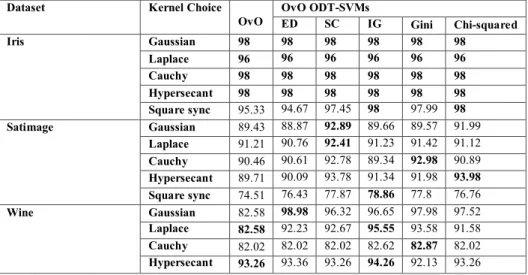
Table 3 and Table 4 show the comparison of maximum classification accuracy between conventional OvO and OvO ODT-SVM, and conventional OAA and OAA ODT-SVMs respectively.
Kernel Function
,
iK x x
for
0
Gaussian) | |
exp( x xi 2 Laplace
|) | exp( xxi Cauchy
(1 (1 |xxi |2))
Hypersecant |)) | exp( |) | (exp(
2 xxi xxi Square sync
2
2 ( | |) ( | |)
sin xxi xxi Table 2: Kernel functions.
Table 5 shows comparison of maximum classification accuracy between both models of ODT-SVM, conventional OvO, conventional OAA and commonly used multi-class classifiers in literature i.e. C45, Multi Layer Perceptron (MLP). C4.5 and MLP implemented in WEKA machine learning environment [26] are used in our experiments with their default values of parameters. The best classification accuracy for each dataset is shown in bold. When we apply the Friedman test, with 7 algorithms and 11 datasets, FF is distributed according to
the F distribution with (7-1) degrees of freedom. The critical value of F(6,10) at the 0.05 critical level is 2.25. FF calculated from the mean ranks is 12.31.
Since 12.31 > 2.25, we can reject the null hypothesis and infer that there exists a significant difference among adversary classifiers.
Dataset Kernel Choice
OvO OvO ODT-SVMs ED SC IG Gini Chi-squared
Iris Gaussian 98 98 98 98 98 98
Laplace 96 96 96 96 96 96
Cauchy 98 98 98 98 98 98
Hypersecant 98 98 98 98 98 98 Square sync 95.33 94.67 97.45 98 97.99 98 Satimage Gaussian 89.43 88.87 92.89 89.66 89.57 91.99
Laplace 91.21 90.76 92.41 91.23 91.42 91.12
Cauchy 90.46 90.61 92.78 89.34 92.98 90.89
Hypersecant 89.71 90.09 93.78 91.34 91.98 93.98 Square sync 74.51 76.43 77.87 78.86 77.8 76.76
Wine Gaussian 82.58 98.98 96.32 96.65 97.98 97.52
Laplace 82.58 92.23 92.67 95.55 93.58 91.58
Cauchy 82.02 82.02 82.02 82.62 82.87 82.02
Square sync 75.28 76.89 76.97 77.97 75.28 76.97
Vehicle Gaussian 76.83 79.95 84.45 84.82 85.24 85.24 Laplace 77.42 78.3 80.61 81.61 80.74 80.24
Cauchy 76.48 82.85 84.52 84.52 84.58 85.65 Hypersecant 83.33 81.59 84.28 84.28 84.98 84.98 Square sync 71.51 80.57 81.32 81.32 81.99 81.56
Glass Gaussian 72.43 62.9 71.5 71.21 69.63 75.43 Laplace 75.70 76.17 76.64 74.64 75.7 77.57 Cauchy 72.90 72.21 72.43 71.03 68.92 73.36 Hypersecant 71.96 72.90 71.5 70.09 69.16 71.03
Square sync 66.36 64.2 64.78 62.62 62.62 56.07
Segmentation Gaussian 84.76 87.85 89.24 89.29 88.87 87.43
Laplace 87.14 88.19 89.62 89.67 89.87 90.87 Cauchy 86.19 91 89.87 89.69 89.71 89.99
Hypersecant 90 89.14 90.87 89.52 92.05 91.95
Square sync 81.9 79.05 79.52 80.13 80.95 79.05
Ecoli Gaussian 85.42 84.98 85.42 86.01 84.79 86.14 Laplace 86.97 87.2 86.99 86.9 86.99 87.9 Cauchy 85.42 85.42 86.98 84.82 86.52 85.71
Hypersecant 85.42 85.42 88.45 88.82 85.42 85.74
Square sync 85.12 84.23 87.65 85.12 87.85 86.15
New_Thyroid Gaussian 97.21 97.21 97.21 100 98.21 97.21
Laplace 96.74 96.74 100 96.89 96.89 96.74
Cauchy 96.74 96.84 100 96.89 96.89 97.74
Hypersecant 97.67 100 98.67 98.89 100 100
Square sync 94.88 94.88 96.49 96.49 96.49 96.49 Yeast Gaussian 58.43 59.92 62.40 60.32 63.95 61.92
Laplace 59.56 60.31 62.43 63.32 65.17 61.86
Cauchy 61.54 62.37 64.17 65.41 66.54 62.54
Hypersecant 59.45 67.76 67.65 67.54 65.56 64.76
Square sync 57.98 57.32 58.68 59.45 60.12 58.98
Movement_Libra Gaussian 74.45 79.94 81.91 78.94 77.74 76.94
Laplace 81.73 83.77 85.77 85.87 87.97 82.77
Cauchy 76.45 78.13 79.89 78.54 76.89 78.89
Hypersecant 72.23 78.64 77.65 73.64 77.18 76.64
Square sync 42.22 42.22 42.22 42.22 42.22 42.22 HeartDisease_Cleveland Gaussian 43.56 41.23 34.87 42.27 12.54 43.56 Laplace 22.11 23.43 23.91 32.31 11.88 22.11
Cauchy 15.23 34.38 17.47 13.45 12.21 15.18
Hypersecant 22.44 24.34 25.32 25.41 12.21 22.44
Square sync 12.78 15.38 12.23 11.23 13.43 12.09
Table 3: Classification accuracy of conventional OvO Vs OvO ODT-SVMs [%].
Dataset Kernel
Choice OAA ED OAA ODT-SVM SC IG Gini Chi-square
Iris Gaussian 96 98 98 98 98 98
Laplace 96 96 96 96.44 96 96
Cauchy 96 98 98 98 98 98 Hypersecant 98 98 98 98 98 98 Square sinc 96 94.67 98 98 98 98 Satimage Gaussian 89.43 88.87 92.89 89.66 89.57 91.99
Laplace 89.95 90.76 92.41 91.23 91.42 91.12
Cauchy 89.46 90.61 92.78 89.34 92.98 90.89
Hypersecant 89.71 90.09 93.78 91.34 91.98 93.98 Square sinc 74.51 76.43 77.87 78.86 77.8 76.76
Wine Gaussian 82.01 98.98 96.32 96.65 97.98 97.52
Laplace 82.58 92.23 92.67 95.55 93.58 91.58
Cauchy 82.15 82.02 82.02 82.62 82.87 82.02
Hypersecant 93.82 93.36 93.26 94.26 92.13 93.26
Square sinc 74.72 76.89 76.97 77.97 75.28 76.97
Laplace 80.61 78.3 80.61 81.61 80.74 80.24
Cauchy 84.52 82.85 84.52 84.52 84.58 85.65 Hypersecant 84.87 81.59 84.28 84.28 84.98 84.98 Square sinc 78.45 80.57 81.32 81.32 81.99 81.56
Glass Gaussian 60.75 62.9 71.5 71.21 69.63 75.43 Laplace 76.17 76.17 76.64 74.64 75.7 77.57 Cauchy 68.69 72.21 72.43 71.03 68.92 73.36 Hypersecant 63.55 72.9 71.5 70.09 69.16 71.03
Square sinc 61.21 64.2 64.78 62.62 62.62 56.07
Segmentation Gaussian 84.36 87.85 89.24 89.29 88.87 87.43
Laplace 86.19 88.19 89.62 89.67 89.87 90.87 Cauchy 85.71 91 89.87 89.69 89.71 89.99
Hypersecant 88.57 89.14 90.87 89.52 92.05 91.95
Square sinc 80.48 79.05 79.52 80.13 80.95 79.05
Ecoli Gaussian 84.01 84.98 85.42 86.01 84.79 86.14 Laplace 86.90 87.2 86.99 86.9 86.99 87.9 Cauchy 86.90 85.42 86.98 84.82 86.52 85.71
Hypersecant 82.74 85.42 88.45 88.82 85.42 85.74
Square sinc 82.74 84.23 87.65 85.12 87.85 86.15
New_Thyroid Gaussian 95.45 97.98 97.54 100 98.21 97.89
Laplace 96.78 98.89 100 98.52 96.89 98.49
Cauchy 97.34 97.65 98.94 97.89 100 97.96
Hypersecant 96.38 100 98.99 98.89 98.90 98.99
Square sinc 93.54 95.56 96.49 96.78 98.67 97.45
Yeast Gaussian 59.65 59.92 63.90 61.54 66.65 62.32
Laplace 61.26 61.43 64.77 65.54 67.65 64.23
Cauchy 59.46 63.23 64.17 67.41 66.54 65.43
Hypersecant 59.99 68.72 68.65 65.54 65.56 61.34
Square sinc 56.54 58.32 58.68 59.45 60.12 59.98
Movement_Libra Gaussian 73.44 77.76 85.21 82.61 76.41 76.34
Laplace 82.48 84.43 84.67 84.42 85.54 83.75
Cauchy 76.14 78.93 74.71 85.54 78.65 78.89
Hypersecant 73.43 77.84 78.45 77.61 78.65 74.64
Square sinc 42.2
2 42.22 42.22 42.22 42.22 42.22 HeartDisease_Cleveland Gaussian 43.43 42.36 44.54 42.51 12.21 43.53
Laplace 29.13 43.03 23.34 31.43 16.78 24.12
Cauchy 45.73 49.38 27.47 43.45 22.35 25.38
Hypersecant 22.44 24.64 27.62 25.32 13.61 21.45
Square sync 12.78 15.48 13.61 11.23 12.43 14.37
Table 4: Classification accuracy of conventional OAA Vs OAA ODT-SVMs [%]. Dataset OvO OAA SVM_BDT OvO ODT-SVM OAA ODT-SVM C4.5 MLP
Iris 98 98 98 98 98 96 97.33
Satimage 91.21 89.95 91.65 93.61 93.98 85.7 88.12
Wine 93.26 96.45 92.63 96.76 98.98 90.96 92.51
Vehicle 83.33 84.87 82.98 84.95 85.65 71.83 81.98
Glass 75.7 76.17 72.69 76.17 77.57 67.61 63.08
Segmentation 90 90 90 93.78 92.05 86.6 90.48
Ecoli 87.97 86.9 85.78 89.98 88.82 85.08 84.34
New_Thyroid 97.67 97.34 100 100 100 91.59 95.33
Yeast 61.54 61.26 68.59 67.65 68.65 56.71 61.43
Movement_Libra 81.73 82.48 87.45 87.97 85.54 67.13 80.78
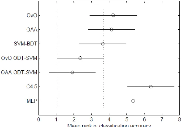
HeartDisease_Cleveland 43.56 45.73 49.43 43.56 49.38 50.33 52.65 Table 5: Comparison of best average classification accuracy of ODT-SVMs with other multi-class classifiers. To determine which classifiers are significantly
different, we carried out Nemenyi test whose results are illustrated in Figure 1. In this figure, the mean rank of each classifier is pointed by a circle. The horizontal bar across each circle indicates the „critical difference‟. The
significantly different from conventional OvO, conventional OAA, SVM-BDT, OAA ODT-SVM in terms of classification accuracy. Rather we can say that the proposed scheme is comparable with all the variants of SVM.
Table 6 and Table 7 shows the computation time of OvO ODT-SVM for training and testing phase respectively for Gaussian kernel with γ = 2-11 and C=1000.Table 6 and Table 7 shows that the time required for training and testing of OvO ODT-SVM is significantly less in comparison to conventional OvO SVM and SVM-BDT approach. Similarly, Table 8 and Table 9 shows that that the time required for training and testing of OAA ODT-SVM is significantly less in comparison to conventional OAA SVM.
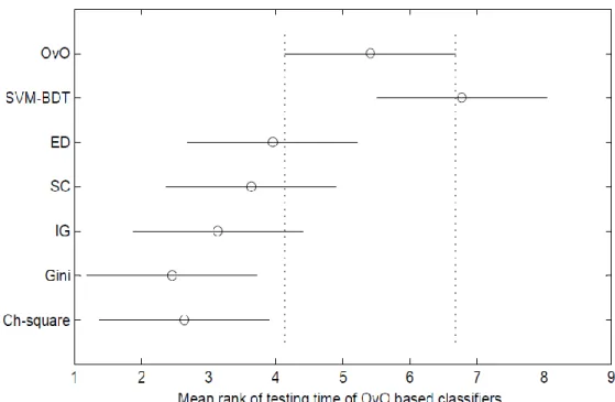
The Friedman test indicates that there exist significant differences among OvO classifiers on both training and testing time.
Figure 2 and Figure 3 illustrate the results of the Nemenyi test to reveal what those differences are among OvO classifiers on training and testing time respectively. Consistent with our time complexity analysis, all variants of OvO ODT-SVM scheme other that Gini measure, are most efficient in terms of training time in
comparison to conventional OvO and SVM-BDT. Figure 3 shows that OvO ODT-SVM using Gini is ranked best and is significantly better than conventional OvO and SVM-BDT. All the variants of OvO ODT-SVM schemes are not significantly different from each other in terms of both training and testing time.
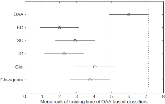
Similarly, the Friedman test indicates that there exist significant differences among OAA schemes on both training and testing time. Figure 4 and Figure 5 illustrate the results of the Nemenyi test to reveal what those differences are among OAA schemes on training and testing time respectively. Again consistent with our time complexity analysis, all variants of OAA ODT-SVM scheme other that gini measure, are most efficient in terms of training time in comparison to conventional OAA. Figure 5 shows that OAA ODT-SVM using IG is ranked best and is significantly better than conventional OAA. Similar to OvO schemes, all the variants of OAA ODT-SVM schemes are not significantly different from each other in terms of both training and testing time Among four measures employed for determining the structure of decision tree, neither of them is clear winner over other in terms of computation time for training and testing.
Figure 1: Apply the Nemenyi test to mean ranks of classification accuracy of various classifiers.
Dataset OvO SVM-BDT OvO ODT-SVM
ED SC IG Gini Chi-square
Iris 2.84 5.18 2.15 2.13 2.19 2.17 2.79
Satimage 1065.06 2852.82 867.71 864.77 873.48 958.32 871.47
Wine 2.15 3.53 1.96 2.08 2.11 2.13 2.05
Vehicle 189.96 508.81 154.76 154.24 155.79 170.92 155.43
Glass 12.31 16.89 8.93 8.60 9.05 10.06 8.99
Segmentation 3.00 5.26 2.20 2.52 2.49 2.45 2.39
Ecoli 26.48 45.90 17.28 24.09 20.07 21.97 17.55
Yeast 245.87 675.43 178.62 176.32 173.34 198.14 189.54
Movement_Libra 534.78 1432.76 433.56 437.76 446.34 476.73 436.42
HeartDisease_Cleveland 8.42 13.23 4.67 6.87 5.43 6.48 6.65
Table 6: Training time OvO ODT-SVM Vs OvO and SVM-BDT [sec].
Dataset OvO SVM-BDT OvO ODT-SVM
ED SC IG Gini Chi-square
Iris 0.03 0.03 0.03 0.01 0.02 0.02 0.02
Satimage 10.44 18.53 9.96 9.32 9.07 7.79 8.53
Wine 0.03 0.06 0.03 0.03 0.03 0.03 0.03
Vehicle 0.44 0. 79 0.43 0. 44 0.43 0. 33 0. 36
Glass 0.04 0.06 0.02 0.04 0.02 0.03 0.02
Segmentation 0.05 0.07 0.04 0.05 0.04 0.05 0.04
Ecoli 0.05 0.06 0.06 0.04 0.04 0.04 0.04
New_Thyroid 0.07 0.09 0.06 0.05 0.06 0.05 0.05
Yeast 0.98 1.79 0.86 0.89 0.86 0.69 0.78
Movement_Libra 5.89 9.89 4.96 4.89 4.43 3.86 4.54
HeartDisease_Cleveland 0.09 0.10 0.05 0.05 0.04 0.05 0.06
Table 7: Testing time OvO ODT-SVM Vs OvO and SVM-BDT [sec].
Figure 3: Apply the Nemenyi test to mean ranks of testing time of OvO classifiers.
Dataset OAA OAA ODT-SVM
ED SC IG Gini Chi-square Iris 28.09 12.13 21.65 12.07 15.95 15.75
Satimage 3451.82 858.09 945.91 940.30 989.37 989.43
Wine 5.20 2.95 2.53 2.51 2.52 2.52
Vehicle 615.65 153.04 168.71 167.71 176.46 453.63
Glass 135.60 22.85 27.18 27.18 69.02 21.34 Segmentation 6.70 2.17 2.53 2.51 4.80 4.82
Ecoli 80.68 23.34 30.02 31.02 78.42 79.80
New_Thyroid 10.34 4.54 4.23 5.67 5.13 5.67
Yeast 1278.76 306.98 367.87 306.76 359.54 567.87
Movement_Libra 1734.41 428.87 472.87 478.24 478.91 456.69
HeartDisease_Cleveland 102.34 24.76 23.43 21.23 32.23 24.54
Table 8: Training time OAA Vs OAA ODT-SVM [sec].
Dataset OAA OAA ODT-SVM
ED SC IG Gini Chi-square
Iris 0.02 0.03 0.01 0.01 0.01 0.01
Satimage 13.95 7.72 9.07 7.59 9.05 7.87
Wine 0.03 0.02 0.02 0.02 0.02 0.02 Vehicle 0.59 0.33 0.39 0.32 0.38 0.33
Glass 0.05 0.02 0.04 0.04 0.03 0.03
Segmentation 0.05 0.04 0.03 0.03 0.04 0.04
Ecoli 0.05 0.04 0.04 0.03 0.04 0.03 New_Thyroid 0.07 0.05 0.05 0.04 0.04 0.05
Yeast 1.28 0.76 0.89 0.66 0.78 0.69
Movement_Libra 6.89 3.78 4.57 3.87 4.56 4.08
HeartDisease_Cleveland 0.05 0.04 0.03 0.04 0.02 0.03
Figure 4: Apply the Nemenyi test to mean ranks of training time of OAA classifiers.
Figure 5: Apply the Nemenyi test to mean ranks of testing time of OAA classifiers
6
Conclusion
In this paper, we evaluate the performance in terms of classification accuracy and computation time of proposed OvO ODT-SVM and OAA ODT-SVM using the statistical measures i.e. information gain, gini index, chi-square and scatter-matrix-based class separability in kernel-induced space. We have also shown theoretically that the computation time of training and testing of both the ODT-SVMs using statistical measures is better in comparison to conventional SVMs. A robust non-parametric test is carried out for statistical comparison of classifiers over multiple data sets.
The results of the experiment on UCI repository datasets indicate that accuracy of our proposed framework are significantly better than conventional OvO SVM, conventional OAA SVM and two widely used multi-class classifiers such as C4.5 and MLP for most of the datasets. Our experimental results also demonstrate that the computation time of proposed ODT-SVMs formulation is significantly less in comparison to conventional SVM and SVM-BDT models.
decision tree, neither of them is clear winner over other in terms of computation time for training and testing.
Acknowledgements
We are thankful to the reviewers for their valuable comments which have led to the improvement of the paper.
References
[1] Allwein, Schapire, R., & Singer, Y. (2000). Reducing multiclass to binary: A unifying approach for margin classifiers .In Machine Learning: Proceedings of the Seventeenth International Conference.
[2] Blake, C. L., & Merz, C. J. (1998). (C. Irvine, Producer, & Univ. California, Dept. Inform. Computer Science) Retrieved from UCI Repository
of Machine Learning Databases:
http://www.ics.uci.edu/~mlearn/ML-Repository.htm [3] Boser, Guyon, I., & Vapnik, V. (1992). A training
algorithm for optimal margin classifiers. 5th Annual ACM Workshop on COLT, (pp. 144-152).
[4] Bredensteiner, & Bennet, K. ( 1999). Multicategory classification by support vector machines . In Computational Optimizations and Applications , 12, 53-79.
[5] Breiman, L., Friedman, J., Ohlsen, R., & Stone, C. (1984). Classification and regression trees. Belmont , CA: Wadsworth.
[6] Corts, C., & Vapnik, V.N. (1995). Support Vector Networks. Machine Learning, 20, 273-297.
[7] Crammer, & Singer, Y. (2001). On the algorithmic implementation of multiclass kernel-based vecto rmachines. Journal of Machine Learning Research , 2, 265-292.
[8] Demsar, J. (2006). Statistical Comparisons of Classifiers over Multiple Data sets. Journal Machine Learning Research, 7, 1-30.
[9] Duda, R. O., & Hart, P. E. (1973). Pattern classification and scene analysis. New York: J. Wiley.
[10]Duda, R. O., Hart, P. E., & Stork, D. G. (2000). Pattern Classification (second ed.). John Wiley & Sons, Inc.
[11]Friedman, M. (1940). A Comparison of Alternative Tests of Sgnificance for the Problem of m Ranking. Annals of Math. Statistics, 11, 86-92.
[12] Friedman, M. (1937). The Use of Rank to Avoid the Assumption of Normality Implicit in Analysis of Variance. Journal Am. Statistical Association , 32, 675-701.
[13]Gjorgji, M., Dejan, G., & Ivan, C. (2009). A Multi-class SVM Classifier Utilizing Binary Decision Tree. Informatica, 33, 233-241.
[14]Hsu, C. W., & Lin, C. J. (2002). A comparison of methods for Multiclass Support vector machine. IEEE Transactions on Neural Networks, 13 (2), 415-425.
[15]Kittler, J., & Hojjatoleslami, A. (1998). A weighted combination of classifiers employing shared and
distinct representations. IEEE Computer Vision Pattern Recognition, (pp. 924-929).
[16] KreBel. (1999). Pairwise classification and support vector machines. Cambridge, MA: MIT Press. [17]Manju, B., & R. K., A. ( july, 210). Statistical
Measures to Determine Optimal Decision Tree Based One versus One SVM. Accepted for publication in Defense Science Journal .
[18] Manju, B., & R. K., A. (2009). Evaluation of Decision Tree SVM Framework Using Different Statistical Measures. International Conference on Advances in Recent Technologies in Communication and Computing, (pp. 341-445). Kerala.
[19]Platt, Cristianini, N., & Shawe-Taylor, J. (2000). Large margin DAGSVM‟s for multiclass classification . Advances in Neural Information Processing System, 12, 547–553.
[20] Quinlan, J. R. (1987). Induction of Decision Trees. Machine Learning, 1, 81-106.
[21]Rifkin, R., & Klautau, A. (2004). In Defence of One-Vs.-All Classification. Journal of Machine Learning, 5, 101-141.
[22]Scholkopf, B., & smola, A. (2002). Learning with kernels. Cambridge, MA: MIT Press.
[23] Shannon, C. E. (1948). A Mathematical Theory of Communication. Bell System Tech. Journal, 27, 379-423, 623-659.
[24]Takahashi, F., & Abe, S. (2002). Decision-tree-based multiclass support vector machines. Proceedings of the Ninth International Conference on Neural Information Processing (ICONIP ’02), 3, pp. 1418– 22. Singapore.
[25]Vapnik, V. N. (1998 ). Statistical Learning Theory. New York: John Wiley & Sons.
![Table 3: Classification accuracy of conventional OvO Vs OvO ODT-SVMs [%].](https://thumb-us.123doks.com/thumbv2/123dok_us/8043544.2129878/7.893.192.719.120.824/table-classification-accuracy-conventional-ovo-ovo-odt-svms.webp)
![Table 4: Classification accuracy of conventional OAA Vs OAA ODT-SVMs [%].](https://thumb-us.123doks.com/thumbv2/123dok_us/8043544.2129878/8.893.208.703.120.790/table-classification-accuracy-conventional-oaa-oaa-odt-svms.webp)